VBIC MODELING HANDBOOK

Transcription

1 -- VBIC MODELING HANDBOOK Keysight Technologies and F.Sischka VBIC Modeling Handbook /3/27

2 -2- Foreword This handbook is an updated and enhanced version of the Keysight Technologies Modeling Handbook, chapter VBIC Modeling.. Note for users of IC-CAP: pls. contact for the corresponding ModelFile VBIC Modeling Handbook /3/27

3 -3- Contents: VBIC Model Introduction... 4 Definitions... 6 Recapitulating the Gummel-Poon Model... 6 The Normalized Base Charge Qb... 7 DC Performance... 8 Resistors... 9 Capacitors... 9 Transit Time... AC SMALL SIGNAL SCHEMATIC... A quick Tutorial on the Gummel-Poon Parameters... 2 Gummel-Poon Model Parameter List... 6 VBIC Model Description... 7 The Normalized Base Charges qb and qbp... 8 Space Charge Capacitors... 9 DC Performance of the Main NPN Transistor... 2 DC Performance of the Parasitic PNP Transistor Resistors Quasi-Saturation Base Widening Diffusion Charge Capacitors Additional Phase Shift: Self-Heating Modeling VBIC Model Parameter List Comparing the VBIC and Gummel-Poon Parameters Converting Gummel-Poon Parameters to VBIC VBIC Modeling Strategy VBIC Parameter Extraction Sequence Space Charge Capacitances Parasitic Resistors From DC Measurements Early Voltages Diode Parameters The Gummel-Plot Modeling of Main and Parasitic Transistor at a Glance: Output Characteristics... 5 The 'foutput' Saturation Range Modeling at a Glance: Small Signal S-Parameter Modeling The Transit Time Modeling at a Glance: Geometry Scaling Modeling Thermal Modeling VBIC Background Information SIMPLIFIED VBIC EQUATIONS, rev...4: Information on the VBIC Code, Release Default Parameters rev Publications... 7 VBIC Modeling Handbook /3/27

4 -4- VBIC Model Introduction The VBIC model is an enhancement to the Spice Gummel-Poon Model. In details: -> Precise implementation of the Base width modulation -> Approximating a distributed Base region -> Parasitic Substrate transistor -> Improved Kull model for quasi-saturation -> Enhanced delay time modeling -> weak avalanche current effects -> consistent treatment of the additional phase factor for small signal and time domain analysis -> improved capacitance model -> includes self-heating and improved model parameter temperature dependence VBIC Model History rev..2 updates Sept. 24, terminal version defined Base-emitter breakdown model added Reach-through model added for B-C depletion capacitance Homotopy version of code added Limited exponential version added Completely new code generation added C, FORTRAN, Verilog-A, Perl, and MAST code provided Bug in psibi mapping with temperature fixed Bugs in electrothermal derivatives and solver stamp fixed DTEMP local temperature difference parameter added VERS and VREV (version revision) parameters added NKF high current beta rolloff parameter added Temperature dependence added to IKF Ability to select SGP qb formulation added (QBM) Ability to separate IS for fwd and rev added (ISRR) Fixed collector-substrate capacitance added (CCSO) Separate temperature coeffs added for RCX, RBX, RBP tl node eliminated POLARITY OF SOME BRANCHES REVERSED FOR VERILOG-A COMPATIBILITY > Ith flows from dt to ground and so is negative > Ixzf flows from xf to ground as so is negative of Itzf Igc component moved into Ibc Icc broken into forward and reverse components, Itxf or Itzf and Itzr..5 updates July 28, 996 Dependence of Irbp on Vbci added to "branch currents" Itf/Itr renamed Itfi/Itri to avoid name conflicts Resistor collapse and code bypass condition changed from par = to par <= Branch current and charge dependencies separated for self-heating and no self-heating VBIC Modeling Handbook /3/27

5 -5Depletion charge and avalanche routines that provide derivatives for self-heating added Self-heating solver and examples added (HBT) Extra external node added for self-heating to allow coupling of thermal models between devices..4 updates Qbe diffusion term made equivalent to SGP (divide by qb) Solver example including excess phase added (Icc separated into ItzfItxf and Itzr for this) Error in sgp_to_vbic in PTF to TD translation fixed..3 updates Ith bug fixed and Igc term added BFN exponent added to /f noise RTH default changed to zero parameter aliases added..2 updates EAI bug fixed in PE/PC/PStemperature mapping Single->double precision in decomp/solve/vbict/qcdepl Scale changed to vscale in solver to avoid name conflict Avalanche model added, element Igc Initialization changed in solver AC solver and AC and temperature tests added Missing term in derf_vrci added Potential numerical problem in Irci fixed.. updates VJ->V bug fixed in qj definition Potential numerical problems with ITF fixed Typo derf_vcci fixed to derf_vrci in FORTRAN code VBIC Modeling Handbook /3/27

6 -6- Definitions Currents are always considered to flow into the device. This means, for example, that IC is a current into the Collector of the transistor. Voltages are indexed with their reference nodes. In order to have a clear notation, voltage drops across parasitic resistors are only considered, if this is required to better understand a specific detail or to prevent from confusion. This means, that vbe stands usually for a voltage between inner Base and inner Emitter vb E. All notations in this handbook are based on an NPN transistor. Recapitulating the Gummel-Poon Model Since the VBIC model is an enhancement to the Gummel-Poon (G-P) model, this chapter recaps its fundamentals. Fig. GP- depicts the Gummel-Poon equivalent schematic large signal model. CB'C' B ib RBB' IC B' C' ib'c' RC C ib'e' CB'E' E' S ic'e' RE E Fig. GP-: Equivalent schematic of the Gummel-Poon large signal model VBIC Modeling Handbook /3/27

7 -7- The Normalized Base Charge Qb The Base majority carrier Base charge normalized to its value without bias is x C e A j p( x ) dx qb QB x E QB x C e A j NA ( x ) dx (GP-) x E qb can be calculated as with 2 q q qb q2 2 2 q QB (GP-2) v BE C je ( V ) dv QB v CE C jc ( V ) dv (GP-3) covering the Early effect (Base width modulation) and v be v bc NF VT q2 IS e IS e NR VT IKR IKF covering the Webster effect (high current behavior). (GP-4) The following simplifications are applied to all common implementations of the G-P model, see e.g. the University Berkeley SPICE version. Equation (GP-2) is approximated by q qb 4 q2 2 and charge q is approximated by v v q bc be v VAF VAR bc v be VAF (GP-5) (GP-6) VAR in order to obtain, similarly to the Ebers-Moll model, a constant output conductance. Besides the approximation +x ~ /(-x) for x<<, equation (GP-6) further assumes constant space charge capacitors. The second approximation in equation (GP-6) can lead to rather big modeling errors at low Early voltages. Therefore, some simulators like ADS of Keysight Technologies allow the user to select between one of these approximations. VBIC Modeling Handbook /3/27

8 -8- DC Performance The G-P Collector current IC is an overlay of a forward and reverse component: v be IS v bc IF IR IS NF VT (GP-7) IC e e NR VT q qb qb b with VT=8.62E-5 * (TEMP ). Base width modulation and high current effects are modeled by the bias-depending Base charge qb, see the above chapter. The Base current is composed of an ideal (Ibei, Ibci) and a non-ideal part (Iben, Ibcn). The latter covers the recombination current, a low-bias effect of Ib (Parameters ISE and ISC). The Base current in forward mode is v be v be IS NF VT Ibe Ibei Iben e ISE e NE v T (GP-8) BF and in reverse mode v bc v bc IS NR VT NC v T Ibc Ibci Ibcn e ISC e. BR (GP-9) Figures GP-2 and GP-3 visualize the most important DC effects covered by the SPICE G-P model. ohmic and high current effects ic(ma) ic 3 Base width modulation BF ib Fig. GP-2: Typical output characteristic recombination effect Fig. GP-3: Gummel plot vb(v). VBIC Modeling Handbook /3/27

9 -9- Resistors The parasitic resistors Re and Rc are assumed to be constant. Rb, however, is modeled bias-dependent. In the SPICE G-P model, it is implemented as tan z z Rb RBM 3 RB RBM (GP-) z tan2 z with z 2 I 2 b 2 2 IRB Ib IRB Capacitors The capacitors between Base and Emitter, as well as between Base and Collector, represent each the space charge (depletion) and diffusion capacitor. Space Charge Capacitors: The space charge capacitors are described by CJE (GP-) CBEi MJE v i VJE To prevent from the pole in equation (GP-) at vi = VJE, a linear continuation of (GP-) is used for voltages vi > FC*VJE. The Base-Collector capacitor Cjc is distributed between inner and outer Base node of the model by (GP-2) CBCi XCJC CBC and (GP-3) CBC x XCJC CBC In addition to the capacitors depicted in fig. GP-, an additional capacitor between Collector and Substrate is added to the SPICE G-P model. This substrate capacitor is either considered to be a constant or is also modeled after equation (GP-). Diffusion Charge Capacitors: The other charge, related to the diffusion capacitors, is given by Qbe TFF IF and for B-C: Qbc TR IR, (GP-4) (GP-5) where IF stands for the Collector->Emitter current, and IR for the Emitter->Collector current, see equation (GP-7). This means for the capacitors VBIC Modeling Handbook /3/27

10 -v be and ic IS Cbe TFF TFF e NF VT vbe qb NF VT (GP-6) v bc ie IS Cbc TR TR e NR VT. vbc qb NR VT (GP-7) Transit Time The transit time TFF is modeled by the empirical equation v bc 2 IF. 44 VTF e TFF TF XTF I ITF F (GP-8) Fig. GP-4 shows the trace of TFF vs. the Collector current Ic with Vbc as secondary sweep. TFF(psec) vce Fig. GP-4: Trace of TFF (Ic, vbc). ic(ma) Since the measured phase shift of Ic can be bigger than what is covered by the model equations, the UCB SPICE G-P model has an additional parameter PTF. Its additional phase shift is added to the phase of Ic. VBIC Modeling Handbook /3/27

11 -- AC SMALL SIGNAL SCHEMATIC From fig. GP-, the small signal schematic for high frequency simulations can be derived. This means, for a given operating point, the DC currents are calculated and the model is linearized in this point, see the figure below. Such a schematic is used for S-parameter simulations. B i B CB'C' =CMU RBB' IC C' B' RC C CC'S' rb'e' R CB'E' =CPI gm*vb'e' E' S RE E Fig. GP-5: AC small signal schematic of the bipolar transistor NOTE: XCJC effect neglected. Note: this schematic is a pure linear model. It cannot be used to predict non-linear high-frequency behavior of the transistor. In order to do this, RF simulators like ADS apply harmonic-balance techniques to perform nonlinear RF large signal simulations. VBIC Modeling Handbook /3/27

12 -2- A quick Tutorial on the Gummel-Poon Parameters This chapter visualizes the G-P parameter effects on the measurements. space charge capacitor modeling CBE (pf).6 p.2 p slope: MJE CJE + Coffs.8 p -3 - vbe (V) VJE FC*VJE Early voltage extraction ic(ma) 3 -VAF vc(v) VBIC Modeling Handbook /3/27

13 -3forward beta parameter extraction ic ib /RE IKF ISE 2,3*NF*vt decade decade 2,3*NE*vt BF vb(v) IS beta BF NE IKF, RE ISE vbe VBIC Modeling Handbook /3/27

14 -4Base resistor parameter extraction extrapolated for infinite frequency rbe j*imag rbb'+/gb'e'+re(+ß) rbb'+re REAL ib frequency this gives: RBB(Ohm) RB IRB RBM RBM IRB ib(a) VBIC Modeling Handbook /3/27

15 -5Transit time parameter determination First model the TFF trace without VCE effect. Calculate ft from the -2dB/decade slope of H2 log (ft) ft = *PI*TFF log (ic) Then, calculate TFF = / (2*PI*fT) TFF(psec) XTF TF(+XTF) Effect of the space charge capacitors ITF TF theoretical curve ic(ma) isothermically measurable range And, finally model the dependence of ft on VCE: log (ft) ft = *PI*TFF vce log (ic) VBIC Modeling Handbook /3/27

16 -6- Gummel-Poon Model Parameter List The following table compiles the G-P model parameters and their SPICE default values. These default values basically switch off the effect covered by these parameters, what enables to simulate a transistor behavior also when not knowing all the model parameters. (Do not confuse the default parameters with typical parameters!) Name Parameter explanation SPICE Unit default typ.value DC: IS transport saturation current.e-5.e-5 A XTI temperature exponent for effect on IS 3 3 EG energy gap for temperature effect on IS.. ev BF BR XTB ideal forward maximum beta ideal reverse maximum beta forward & reverse beta temp.coeff. VAF VAR forward Early voltage reverse Early voltage NF NR NE NC forward current emission coeff. reverse current emission coeff. B-E leakage emission coeff. B-C leakage emission coeff. ISE ISC B-E leakage saturation current B-C leakage saturation current IKF IKR forward beta hi current roll-off reverse beta hi current roll-off OHMIC PARASITICS: RB zero bias base resistance IRB current at medium base resistance RBM min.base resistance at hi current RE emitter resistance RC collector resistance infinite infinite E-2.E-3 A A infinite infinite.5.3 A A infinite RB CBE: CJE B-E zero-bias deplet.capacitance VJE B-E built-in potential MJE B-E junction exponential factor CBC: CJC B-C zero-bias deplet.capacitance VJC B-C built-in potential MJC B-C junction exponential factor XCJC fraction of B-C capacitor connected to int.base CCS: CJS zero-bias collector-substrate capacitance VJS substrate junction built-in potential MJS substrate junction exponential factor CAPACITOR FORWARD CHARACTERISTICS: FC forward bias depletion cap.coeff. TRANSIT TIME: TF ideal forward transit time XTF coeff.for bias dependence of TF VTF voltage describing VBC dependence of TF ITF hi-current parameter for effect on TF PTF excess phase at frequency /(TF*2PI) TR ideal reverse transit time NOISE: KF flicker noise coeff. AF flicker noise exponent V V Ohm A Ohm Ohm Ohm E F V E F V.75 F V.5.5 infinite.e-2 sec 5 V 2.E-3 A deg 5.E-2sec VBIC Modeling Handbook /3/27

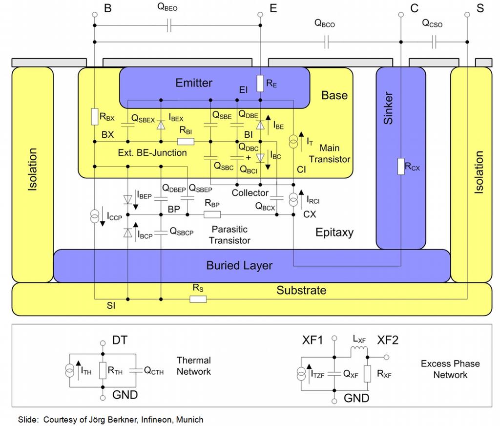
17 -7- VBIC Model Description Fig. VBIC- shows the complete equivalent schematic of the VBIC model. Besides the main NPN transistor between Base, Collector and Emitter, there is an additional parasitic PNP transistor between Base, Collector and Substrate. An additional circuit is added to cover self-heating (Rth,Cth). Also, an extra circuit for adding phase shift to Icc is available. The resistances Rc, Rbi/qb and Rbip/qbp are modeled non-linearily. S C B E S self-heating Ith CBCO Rs Rth Cth Ibcnp Rcx Ibcip Cjcp Ibeip Cbep Cjep Cx Rbip/qbp Icp add'tl phase shift Itzf Llxf Ccxf C Rc Ibenp Cbcx B Rbx Bx Cbcq Cjc Cbc Ibcn Rbi/qb Ibexn Ibexi Icc Bi Iben Cje Cjex CBEO Ibei Cbe Ei Fig. VBIC-: Equivalent schematic of the VBIC model Ibci - Iaval Re E A note on the current flow direction of the ICP source of the parasitic PNP. As can be seen from the main NPN transistor, the transport current is always in the same direction like its driving currents, i.e. the diode currents Ibei and Iben. For the parasitic PNP, this has to be true also: flowing from its Emitter to the Collector (what is the common forward operating condition for a PNP!). VBIC Modeling Handbook /3/27

18 -8We will now look into the details of the VBIC formulation. Thermal effects will be neglected. Currents will be indexed with their corresponding node names and flowing into the nodes. Voltages, indexed by their two node names, will additionally be named by abbreviations like i for internal, x for external, o for outer and p for parasitic. The following formulas refer to VBIC rev...4 The Normalized Base Charges qb and qbp Since the VBIC's major root is the Gummel-Poon model, it is again the Base charge qb, which is one of the most important internal model parameters. However, with the VBIC, approximations like in the SPICE G-P model are not used at all. As a consequence, this allows a bias dependent modeling of the output conductance gce! The charge qb is implemented as 2 q q qb q2 2 2 with q as a function of the space charge capacitors q je q jc q VER VEF (VBIC-) (VBIC-2) (different from the SPICE G-P model, see eqn. (GP-6) and v bei v bci IS e NF VT IS e NR VT. IKR IKF with the temperature voltage VT=8.62E-5 * (TEMP ). q2 (VBIC-3) qje and qjc are the normalized charges of the space charge (depletion) capacitors Cje and Cjc. This implies that the space charge capacitors have to be modeled before the Early voltages are extracted! For the parasitic PNP transistor, its Base charge qbp is given by qbp 4 q2p 2 yet neglecting the Early effect! The charge (VBIC-4) Itfp (VBIC-5) IKP covers the Webster effect of the parasitic PNP transistor, but only in forward bias mode. q2p VBIC Modeling Handbook /3/27

19 -9- Space Charge Capacitors The Base-Emitter space charge capacitance is given for vbe < FC*PE by CJE CSBE M vbe E PE and else CJE v CSBE * FC * ME ME * BE PE FC ME (VBIC-8) (VBIC-9) The same formula applies also to the other space charge capacitor CSBC, and the ones of the parasitic PNP. For these space charge capacitors, there is, besides this SPICE G-P formulation, also an alternate continuous formula implemented in VBIC. This alternate method requires no linear continuation in order to avoid the pole in the SPICE-like equation. The model parameters AJx with x=c, E or S, select the preferred model (-.5, the default VBIC implementation, selects the G-P linear continuation formula). The Base-Emitter space charge capacitance is, in analogy to the partitioning of the Base-Emitter current by the DC parameter WBE (see further below), distributed between internal and external Base. The Base-Collector space charge capacitance is distributed between the capacitances Cjc (Base and Collector of the main transistor) and Cjep (Base and Emitter of the parasitic one). Another space charge capacitance, Cjcp, is located between Base and Collector of the parasitic PNP. It corresponds to the substrate capacitance in the SPICE G-P model. VBIC Modeling Handbook /3/27

20 -2- DC Performance of the Main NPN Transistor NPN Collector-Emitter Current: The Collector current source ICC is determined, similar to the SPICE G-P model, by the forward and reverse transport current terms ITF and ITR: v IS ISRR vbci ITF ITR IS NFbei VT NR VT Icc e e qb qb qb (VBIC-) with the temperature voltage VT=8.62E-5 * (TEMP ). This means that the Collector-Emitter current in forward operation is given by IS Ice qb vbei NF VT e (VBIC-) and in reverse operation by v IS ISRR NRbci Iec e VT qb (VBIC-2) with the reverse saturation current correction factor ISRR = [... inf) VBIC Modeling Handbook /3/27

21 -2NPN Base-Emitter Current: Like with the SPICE Gummel-Poon model, the Base-Emitter current covers the ideal and non-ideal (recombination) behavior. However, with the VBIC model, it is not coupled to the Collector current ICC like with the Gummel-Poon model, where we have the model parameters BF and BR. Here, two separate, parallel diode currents are used instead, one for the ideal part (index I ) and the other for the non-ideal part (index N) of the Base-Emitter current: Ibe Iben Ibexn Ibei Ibexi v bei v bei IBEN e NEN VT IBEI e NEI VT (VBIC-3) Note: the VBIC parameter naming is very mnemonic: I ideal part of the Base current N non-ideal part of the Base current X external part of the Base current The VBIC model features a split of the Base-Emitter current 'to the right and to the left' of the internal Base resistor RBI. This means that the very inner Base-Emitter current from node 'Bi' to 'Ei' is given by (VBIC-4) Ibe _ int ernal Iben Ibei WBE Ibe and the outer Base-Emitter current from the node 'Bx' to 'Ei' is given by Ibe _ external Ibexn Ibexi WBE Ibe (VBIC-5) NOTE: WBE, does not affect the DC fitting, but the S-parameter fitting instead. NPN Base-Collector Current: The Base-Collector current is calculated in analogy to (VBIC-3): v bci v bci NCN VT Ibc Ibcn Ibci IBCN e IBCI e NCI VT (VBIC-6) The Avalanche Current in VBIC is described by ibc _ avalanche Icc Ibc AVC PC Vbci exp AVC2 PC Vbci MC (VBIC-7) It overlays the current ib(vce), and also shows up in the forward output characteristics ic vs. vce. VBIC Modeling Handbook /3/27

22 -22- DC Performance of the Parasitic PNP Transistor PNP Collector-Emitter Current: The current Icp of the parasitic PNP transistor, again, is the difference between the forward and reverse transport currents Itfp and Itrp. Itfp Itrp. (VBIC-8) Icp qbp However, the control of the forward transport current Itfp is split into the voltages vbci of the NPN and vbep of the parasitic PNP transistor: v bep v bci (VBIC-9) Itfp ISP WSP e NFP VT WSP e NFP VT The parameter WSP controls that splitting. Its default value is. With WSP=, a second knee in the log(ib) vs. vce and log(is) vs. vce is modeled, with WSP=, the log(ib) and log(is) drop in a single step. The parasitic PNP reverse transport current is defined by v bcp NFP VT Itrp ISP e Note once again the VBIC mnemonic: P parasitic PNP transistor (VBIC-2) PNP Base-Emitter Current: The Base-Emitter current is, like with the main NPN, split into an ideal and non-ideal part in forward and reverse operating mode. v bep v bep (VBIC-2) Ibep IBENP e NCN VT IBEIP e NCI VT Important note: since the parasitic Base-Emitter is identical to the Base-Collector of the main NPN transistor, the reverse emission coefficients of the MAIN NPN, i.e. NCN and NCI, are also used for the parasitic forward Base current formula! PNP Base-Collector Current: Finally, the Base-Collector current for reverse operation of the PNP is v bcp v bcp NCIP VT NCNP VT Ibcp IBCIP e IBCNP e (VBIC-22) VBIC Modeling Handbook /3/27

23 -23- Resistors The parasitic resistors RE of the Emitter and RS of the Substrate contact are modeled with a constant value. The Base resistance RB, however, is comprised of a constant part RBX and a variable part RBI/qb Rb = RBX + RBI/qb (VBIC-23) with qb after equations (VBIC-)..(VBIC-3) The parasitic PNP Base resistance, RBIP is modeled by Rbi,eff = RBIP/qbp (VBIC-24) with qbp after equations (VBIC-4)..(VBIC-5) The Collector resistance RC, different to the G-P model, now consists of a constant part RCX and a current-dependent, non-linear part RCI, modeling the quasi-saturation region. The constant RCX fits the low bias ic-vce output characteristics at low vbe, as shown below: RCX RCI eff. VBIC Modeling Handbook /3/27

24 -24- Quasi-Saturation Quasi-saturation, as implemented in VBIC, is essentially based on the Kull model. This means that the current through the resistor RCI is depending on the inner and outer Collector voltage. With some smaller modifications to the Kull model, which essentially refer to the modeling of the velocity saturation at high voltages, the current Irci_eff through resistor RCI is given by Irci _ eff Irci Irci RCI 2.5 Vrci. V V HRCF 2 (VBIC-25) In order to better understand this complex formulation, we consider its terms individually: For low vbe,, the slope of ic-vce, is determined, like with the Gummel-Poon model, by the external Collector resistor RCX. For higher vbe bias levels, the internal resistor RCI comes into play. This resistor RCI is bias dependent, while RCX is not. The bias dependency of RCI is related to both, the voltage drop across it, plus the current thru it. Let's start with the Ohmic law, applied to RCI and considering vrci = vcx - vci. v Vcorr Irci _ eff rci RCI (VBIC-26) This means, the voltage drop across RCI is depending on a correction voltage. For non-saturated bias, Vcorr =, and the internal Collector resistor is constant and equal to RCI. When quasi-saturation occurs, Vcorr >, what means that Irci increases. The effective internal Collector resistor is therefore reduced! This correction voltage is given by K bci Vcorr VT K bci K bcx ln K bcx with the coefficients K bci and K bcx v bci GAMM e VT v bcx GAMM e VT (VBIC-27). (VBIC-28) VBIC Modeling Handbook /3/27

25 -25- VT with k * TNOM q (VBIC-29) k 8.67E 5 q In addition to this reduction of the effective, internal Collector resistor, its value can further be reduced due charge carrier velocity saturation, and we obtain equation VBIC-25 from above. Simplified for HRCF -> infinite, VBIC-25 reduces to Irci _ eff Irci I RCI rci V 2 This simplification shows that Irci_eff is reduced for increasing values of Irci if Irci RCI > VO. VBIC Modeling Handbook /3/27

26 -26- Base Widening The additional charge caused by quasi-saturation (Base widening), also influences the dynamic behavior of the transistor (S-parameter). This is covered by parameter QCO which models the charges stored with the capacitances Cbcx and Cbcq. Therefore, QCO affects the ft modeling for low vce, i.e. in quasi-saturation. Q bcx QC K bcx Q bcxq QC K bci (VBIC-3) (VBIC-3) with Kbcx and Kbci from (VBIC-27) and (VBIC-28). Diffusion Charge Capacitors Diffusion Charge Capacitors of the NPN Transistor: The diffusion capacitance of the main transistor are modeled like in the G-P model. The charge, stored in the capacitors Cbe and Cbc, is calculated by Q be TFF I F and for B-C: Q bc TR I R. (VBIC-32) (VBIC-33) The forward transit time is calculated by 2 v bci IF. 44 VTF e TFF TF QTF q XTF IF ITF (VBIC-34) The term (+QTF q) covers additionally a dependency of the Base width modulation. Diffusion Charge Capacitors of the PNP Transistor: Related to the parasitic PNP transistor, the model features only one diffusion capacitance Cbep, which is described by Q bep TR I fp (VBIC-35) VBIC Modeling Handbook /3/27

27 -27- Additional Phase Shift: The additional phase shift is calculated with the VBIC model by a separate network. From the parameter TD, the phase is generated by a Bessel function of second order. The advantage of this method is essentially the consistent description of additional phase in the small signal and transient analysis. TD can be extracted from the phase of H2 of the TFF measurement. However,be careful when applying TD: the S-parameter shapes can easily exhibit unphysical resonances, if TD is too large. Self-Heating Modeling Different to the Spice Gummel-Poon model, the temperature is no longer a static environment parameter in VBIC. Based on the additional temperature network consisting of the thermal resistor RTH and the temperature time constant RTH*CTH, the actual, bias-dependent temperature conditions of the transistor are reflected. VBIC Model Parameter List Compared to the SPICE Gummel-Poon model, VBIC hosts a lot more parameters. But, keep in mind that the naming of the VBIC parameters is really very mnemonic: I ideal part of the Base current N non-ideal part of the Base current, recombination effect, below the 'knee' P a model parameter of the parasitic PNP With this in mind, the VBIC can be understood very easily with its similarity to the G-P model! VBIC Modeling Handbook /3/27

28 -28VBIC Parameter Default Value Parasitic Capacitors CBE CBC Space Charge CapacitorsIBCN CJE PE.75 ME.33 AJE -.5 CJC PC MC AJC CJEP CJCP PS MS AJS FC Early Modeling VEF VER DC Forward IS NF IBEI NEI IBEN NEN IKF Quasi -Saturation RCI GAMM VO HRCF QCO Time Delay Modeling TF QTF XTF ITF VTF TR.9 k k.f a 2 m k k Excess Phase Delay Time TD Flicker Noise AFN BFN KFN Parameter DC Reverse NR IBCI NCI NCN IKR Default Value Distributed Base WBE.f 2 Parasitic Transistor ISP WSP NFP IBEIP IBENP IKP IBCIP NCIP IBCNP NCNP 2 Avalanche Effect AVC AVC2 Resistances RE RBX RBI RS RBP RCX m m m m m m Temperature Modeling CTH * RTH TAMB 27 TNOM 27 EA.2 EAIE.2 EAIC.2 EAIS.2 EANE.2 EANC.2 EANS.2 XRE XRBI, XRBX XRCI, XRCX XRS XVO XIS XII XIN TNF TAVC IMPORTANT NOTE: if RTH is specified, do not set CTH= (the common default value). In this case, the transistor would be thermally faster than electrically!!! VBIC Modeling Handbook /3/27

29 -29- Comparing the VBIC and Gummel-Poon Parameters The table below gives a comparison between the VBIC and the G-P model parameters. VBIC G-P Remarks. Parasitic Capacitors CBE External capacitors, not included in the G-P model CBC External capacitors, not included in the G-P model Space Charge Capacitors AJE AJE selects one of the space charge models (-.5 for G-P version) CJE CJE PE VJE ME MJE AJC CJC PC MC AJC selects one of the space charge models (-.5 for G-P version) CJC * XCJC VJC MJC CJEP CJC*(-XCJC) CJCP PS MS AJS CJS VJS MJS - GP only includes the CV path from C->S, however not the DC C->S diode FC FC Default for VBIC:.9; at G-P:.5 WBE - WBE distributes the Base-Emitter current space charge capacitor between inner and outer Base Early Modeling VEF VAF VER VAR AJS selects one of the space charge models (-.5 for G-P version) The Early effect is modeled differently With the VBIC model!! DC Forward Main Transistor IS IS NF NF Forward Base: IBEI IS / BF NEI NF IBEN ISE NEN NE IKF With the VBIC, the forward Base current is not coupled to the Collector current. Instead, two parallel diodes, one to model the ideal (I) Base current and another to cover the non-ideal or recombination (N) effect, are used. IKF VBIC Modeling Handbook /3/27

30 -3- VBIC G-P Remarks. DC reverse Main Transistor NR IBCI NCI IBCN NCN IKR NR IS / BF NR ISC NC IKR Note: IS from the forward Collector current model is used. With the VBIC model, the reverse Base current is not coupled to the Emitter current. Instead, two parallel diodes, one to model the ideal (I) Base current and another to cover the non-ideal or recombination effect (N) effect, are used. Parasitic Transistor ISP G-P does not cover a parasitic transistor NFP WSP Distributes parasitic collector current control to vbci of the main transistor and vbep of the parasitic transistor Forward Base: BEIP IBENP - For the exponential coefficient, NCI of the main transistor is used For the exponential coefficient, NCN of the main transistor is used Reverse Base IBCIP NCIP IBCNP NCNP - With the VBIC model, the reverse Base current is not coupled to the Collector current. Instead, two parallel diodes, one to model the ideal (I) Base current and another to cover the non-ideal or recombination effect (N), are used. IKP - Avalanche Effect AVC AVC2 Resistances RE RE RBX RBM The bias-dependent Base resistance is modeled differently RBI RB - RBM in both models. RB IRB RS RBP RCX RC Constant, external Collector resistance VBIC Modeling Handbook /3/27

31 -3- VBIC G-P Quasi-Saturation CI GAMM VO HRCF QCO - Remarks. VBIC has a modified Kull model implemented Transit Time Modeling TF TF QTF Describes the additional dependency of the transit time from qb. XTF XTF ITF ITF VTF VTF TR TR Excess Phase TD *TF*PTF/8 The VBIC implementation is consistent between small signal and transient analysis Temperature Dependence CTH VBIC includes self-heating effects RTH TAMB Environmental temperature TNOM TNOM Measurement temperature for parameter extraction EA EG The G-P model only contains one energy gap EAIE EAIC EAIS EANE EANC EANS XRE XRB XRC XRS XVO XIS XII XIN TNF TAVC XTI XTB XTB - Temperature coefficients of the resistors are not covered with G-P VBIC Modeling Handbook /3/27

32 -32- Converting Gummel-Poon Parameters to VBIC Since the VBIC model is based essentially upon the G-P model, most of the G-P parameters can be converted to VBIC. However, the following details have to be kept in mind: Space Charge Capacitances For all space charge capacitances, the parameter Ajx with x = E, C and S must be set to a value less than or equal zero, in order to obtain the same formulation in both models. In this case, the values of the Base-Emitter capacitance can be transferred. With the CJC parameter of the Base-Collector capacitance, it must be reflected that VBIC XCJC CJC GP CJC VBIC XCJC CJC GP and CJEP If the actual SPICE implementation of the G-P model only contains a constant value for the Substrate capacitance, CJCP will hold that value and MS is set to. Finally, FC, modeling the transition between the hyperbolic formulation and the linear continuation, has different default values in both models. Diode Currents The forward and reverse parameters IS, NF and NR can be transferred directly. The ideal Base current sections are not coupled to the transport currents. For VBIC, there is IBEI = IS/BF and IBCI = IS/BR. The G-P parameters of the non-ideal or recombination section of the Base current can, however, be transferred directly to VBIC. Finally, setting WBE =, the Base current distribution (inner and outer Base) is switched off. Early Modeling The implementation of the Early effect in the Gummel-Poon and the VBIC model is so different, that the parameters cannot be converted (different modeling of the normalized Base charge qb). Especially with small G-P Early voltages, the resulting error can be considerably big. Yet, as a general rule, the G-P Early parameters are usually bigger than those of the VBIC model. For rather big values of the G-P Early voltage, only slight modifications should be required. Parasitic Transistor and Avalanche effect Using the mentioned default values in VBIC, the parasitic transistor and the Avalanche effects are switched off. Exception: Base-Collector space charge capacitance. Resistances The constant resistors of Emitter and Collector can be overtaken. From the parameters RBM, RB and IRB of the G-P model, suitable values have to be generated for the VBIC parameters RBI and RBX, since the models differ here. Quasi-Saturation Using suitable parameter values, no quasi-saturation effects are taken into account with the VBIC. Setting GAMM =, Rc is reduced to an ohmic resistance. QC = eliminates the influence of the additional capacitances Cbcx and Cbcq. Transit Time Parameters Setting QTF =, the G-P parameters of the transit time TFF as well as the excess phase can be transferred without any change. Temperature Modeling Setting Rth =, the VBIC temperature model including self-heating is reduced to G-P, which only covers a constant ambient temperature. VBIC Modeling Handbook /3/27

33 -33- VBIC Modeling Strategy For a good modeling result, it is important to follow a certain sequence of extractions, since most model parameters depend on each other. Usually, the first extracted parameters are those, which do not or only lightly depend on others. Then, when proceeding through the extraction strategy, the more nested parameters are extracted subsequently, and the model fits more and more accurately. Related to the VBIC model, the following parameter extraction sequence is proposed. CV: Since the Base charge is the basic relationship of the VBIC Early effect description, it is the space charge capacitors which have to be modeled first. DC: First, the ohmic parasitics RE, RCX and RS are extracted from specific measurement setups. Then, the Early voltages are extracted from the DC output characteristics for non-quasisaturation and no avalanche effect. The parameters, however, are not yet optimized. This is due to the fact that the other DC parameters are not yet know. The Early parameters will be optimized after the fitting of the Gummel plots. The diode parameters ISx and Nx as well as the knee currents IKx of the main NPN transistor are extracted from forward and reverse Gummel-Poon measurements. The transistor should not be in quasi-saturation. From measurements with either an open Emitter contact, or vec= for the main NPN, the diode parameters ISx and Nx and the knee current IKP of the parasitic PNP transistor are extracted. The quasi-saturation parameters, except QC, are calculated from the output characteristics ic(vce, vbe), as well as the avalanche parameters, and the selfheating parameter RTH DC Finetuning: The output characteristics, especially the quasi-saturation region fitting, is fine-tuned by optimization. S-Parameters: The Base resistance is modeled by RBB'=RBX + RBI/qb. Since qb represents a quite complex formula (see equ.(vbic- ff.), the 'input-impedance-circle method' from the Gummel-Poon model cannot applied easily to get a starting value for the inner Base resistance RBI. Therefore, RBI is obtained by optimizing the S plot at high frequencies. The transit time parameters TF, XTF, ITF, VTF are extracted from S-parameter measurements at a fixed frequency for which H2 falls with 2dB/decade_frequency, at non-quasi-saturated bias conditions. Since the dynamic model description for this bias conditions are identical to the SPICE Gummel-Poon model, the same extraction VBIC Modeling Handbook /3/27

34 -34strategy is applied here too. For this condition, we set QTF= The S-parameter quasi-saturation parameter QCO, which affects the high frequency performance, is determined from S-parameter measurements under quasi-saturation DC bias condition. This is done at highest vbe, including the saturated vce bias condition. S-Parameter Finetuning: The S-parameter fitting for all DC bias conditions is fine-tuned using optimization. VBIC Parameter Extraction Sequence Space Charge Capacitances CJx, Mx, Px, AJx, FC The space charge capacitances are determined from CV measurements between Base-Emitter, BaseCollector and Base-Substrate. Since we will use the G-P description, the parameters AJE, AJC and AJS have to be set to -.5 (default!). Note: the trace of C(v) for v>pj does not influence the S-parameter fitting, because the diffusion capacitance (parameters TF, ITF, XTF and VTF) usually overlay the space charge capacitance at this bias condition. We will now refer to the modeling of the BE capacitance. The BC and CS capacitors are modeled correspondingly. For the CV-measurement of the Base-Emitter capacitance, the Collector and Substrate are connected to ground. VBIC Modeling Handbook /3/27

35 -35Measurement Setup: Measurement result and extraction techniques. (pf) C BE.6p.2p slope: MJ open CJE.8p C(v) -3 - CV meter. FC*PE PE vbe (V) Measuring and modeling the Base-Emitter capacitance NOTE on the DC bias for the CV measurements: Rule of thumb: To avoid saturation of the LCRZ meter, the capacitance should only be measured up to a bias voltage at which the capacitance is 2 to 3 times the zero bias capacitance. Stay below of FC*VJ. Note that the default FC for VBIC is.9, rather than the.5 of Spice Gummel-Poon. The behavior of the space charge capacitor is given by equations (VBIC-8) and (VBIC-9): For vbe < FC*PE, we have CJE CSBE M v E BE PE and else CJE v CSBE * FC * ME ME * BE PE FC ME with CJE : space charge capacitance at vbe = V PE : built-in potential or pole voltage (typ.,7v) ME : junction exponential factor, determines the slope of the cv plot FC : forward capacitance switching coefficient, default,9 (CV-) (CV-2) (abrupt pn junction (<,5um): ME = /2) (linear pn junction (> 5um): ME = /3) VBIC Modeling Handbook /3/27

36 -36Determination of the CV parameters: For simplicity, we only use the measurement data from the negative bias, i.e. we begin with the equation (CV-): CJE CSBE M v E BE PE A logarithmic conversion yields: ln(csbe) = ln(cje) - ME ln[ - vbe / PE ] (CV-3) This equation can be interpreted as a linear function according to the ideas of linear regression analysis: with y = y + m * x y = ln(csbe) and (CV-4) y = ln(cje) (CV-5) m = - ME (CV-6) x = ln[ - vbe / PE ] (CV-7) Linear regression means to fit a line to given measurement points. The three parameters obtained by the fitting are y=f(xi,yi) and m=f(xi,yi), together with a fitting quality factor r²=f(xi,yi). For a good fit, r²~ How to proceed: The measured values of CSBE are logarithmically converted according to (CV-4). Following (CV7), the stimuli data of the forcing voltage vbe are nonlinearily converted too. This is done using a starting value for the unknown parameter PE (e.g.,2v). These two arrays are now introduced into the regression equations as corresponding yi- and xi-values. A linear curve is fitted to this transformed 'cloud' of stimulating and measured data, and we get the y-intersect y(pe) and the slope m(pe) for the actual value of PE. In the next step, this procedure is repeated with an incremented PE, and we get another pair of 2 y(pe) and b(pe). But now the regression coefficient r will be different from the earlier one. I.e. depending on the actual value of PE, the regression line fits better or worse the transformed data 'cloud'. Once the best regression coefficient is found, the iteration loop is exited and we finally get PE_opt as well as the corresponding y(pe_opt) and m(pe_opt). Thus we get from (CV-6): ME = - m(pe_opt) and from (CV-5): CJE = exp [ y(pe_opt) ] After that, we apply the same methodology to the other two CV curves. VBIC Modeling Handbook /3/27

37 -37Note: The Base-Collector capacitance is distributed between intrinsic and extrinsic transistor. The main part of this capacitance is usually associated with the parasitic transistor (default settings CJC=.5*CBC_total and CJEP=.95*CBC_total). From the C(v) measurements, however, the partitioning cannot be fine-tuned. This is done with the S-parameters. Basically, the partitioning affects the knee in S22, but also the magnitude of S2 for higher frequencies. Parasitic Resistors From DC Measurements RE Measurement Setup: vc E (m V ) Measurement result: 5 ic= 3 RE vce ib. RE v CE i B 2 ib (m A ) transformed measured data:. visu_re RE Measurement of the open Collector voltage ('flyback method') and the transformed measurement data in the RE domain (delta(vce) / delta(ib)) Extracting the parameters: The ohmic emitter resistor is physically located between the internal Emitter E' and the external Emitter pin E. When we apply a Base current and have the Emitter pin grounded, we get a voltage VBIC Modeling Handbook /3/27

38 -38at the open Collector that is proportional to the Base current through this Emitter resistor. For this measurement, we leave the substrate contact open. We then derivate vce with respect to ib, and get the equivalent RE for each operating point. The result is displayed in a separate plot. The value of RE is then the mean value of the flat range in this plot. RBX An interesting method to determine RBX is to use the RE-flyback method, with additionally measuring vbe /T.Zimmer/. This method is as follows: (vbe-vce) ib ic= vce ib RBX=27 Ohm vbe /ib Measurement Setup and determination of RBX out of transformed measured data. The theoretical values of the measured voltages are: vce = VT * ln(/ai) vbe = ib * RE with and + ib * RE AI: reverse current amplification in common Base + ib * RBX + vb'e' Subtracting these equations and dividing by ib yields: vbe - vce ib = const ----ib + RBX i.e. after plotting the measured data accordingly, we get RBX as the y-intersect. In a parameter visualization step, we apply a loop to these data, in which a line is fitted to two adjacent points, and the local y-intersect is calculated. The incremental y-intersects are then VBIC Modeling Handbook /3/27

39 -39displayed against the stimulus ib, and represent RBX vs. ib. RBX is extracted from the most constant range in this plot. NOTE: RBX may also be obtained from a flyback measurement on the parasitic PNP with ie_main =, i.e Emitter pin of the MAIN transistor left open. RBI Note: RBI is modeled using S-parameters. See further down. VBIC Modeling Handbook /3/27

40 -4- RCX RCX is extracted from the slope of 'is' of the Gummel-Poon plot. The method is after the Isub-method in: J.Berkner, "A Survey of DC-Methods for Determining the Series Resistances of Bipolar Transistors including the New delta-isub Method", Proceedings of the European IC-CAP user meeting 994, Colmar, France Referring to two values of is and ic at two voltages vbe, for which is rises linearily on a LOG(iS)vs.vBE plot, RCX is approximately I VT ln S IS2 RCX IC IC2 As an example, here a Gummel-Poon plot including is: Following the formula above, RCX can be extracted from the transformed, linear range of LOG(iS)vs.vB, as shown below: VBIC Modeling Handbook /3/27

41 -4- RCI This parameter, together with VO, GAMM and HRCF, models the quasi-saturation region of the ic-vce (vbe) plot. It will be modeled after the Gummel-Plot has been fitted. See further down. RS From the reverse Gummel plot of the parasitic transistor, the substrate resistor Rs can be extracted. It is visible as a decline of the slope for high currents. RS is tuned-in and optimized in the parasitic reverse Gummel setup. VBIC Modeling Handbook /3/27

42 -42- Early Voltages VEF, VER When extracting the VBIC Early voltage parameters, their interaction with the space charge capacitances must be considered. Referring to publication C.C.McAndrew, L.W.Nagel, "Early Effect Modeling in SPICE", IEEE Journal of Solid-State Circuits, vol. 3, Nr., Januar 996, equ.9 we start with c jc c je gof gor VEF VEF and q je q jc q je q jc IC IE VER VEF VER VEF with gof, gor output conductance in forward and reverse mode qje, qjc normalized charges cje, cjc normalized capacitances VEF, VER Early voltages These two equations can be rearranged into: a b VEF VER with c d VEF VER a q jc b q je IC c jc gof c q jc d q je They can be solved for the Early voltages and we get: a*d a*d c b b c VEF VER a d c b IE c je gor The operating point has to be selected so that no quasi-saturation or high-current effects (avalanche or thermal) disturb the measured data. Note: VER is often quite low. It is approximately VER ~ VEF * CJC / CJE and CJC is a lot less than CJE in "normal" BJTs because the B-C doping is a lot less than the B-E doping. VBIC Modeling Handbook /3/27

43 -43- Diode Parameters The DC parameters of the Base and Collector current of the main NPN transistor are determined from Gummel-Poon measurements. Referring to the figure below, the parameters are extracted from their dominant bias sweep ranges using regression techniques or visual extraction techniques. The following graphic depicts the basic strategy: IKF NF NEI IS IBEN IBEI NEN Determining the forward Gummel-Poon parameters of the main transistor. The extraction of the IS, NF, IBEx and NEx parameters of the VBIC model is probably the most tedious task in the whole modeling process. Because this 'diode fitting' has to be applied to both, the ic and ib in both, forward and reverse operation, and additionally also once again to the parasitic PNP transistor, it can become a bit confusing. Therefore, it is most important to always remember the VBIC nomenclature: I N P ideal part of the Base current non-ideal part of the Base current parasitic PNP With this in mind, the modeling of the different diode currents becomes much more transparent. Because of this repetitive task, we refer here only to the ic(vbe) modeling of the main NPN transistor. And this methodology can then be applied to all the other parameters like: NPN forward: NPN reverse: PNP forward: PNP reverse: IS, NF, IBEI, NEI, IBEN, NEN, IKF NR, IBCI, NCI, IBCN, NCN, IKR ISP, NFP, IBEIP, IBENP, IKP IBCIP, NCIP, IBNCNP, NCNP VBIC Modeling Handbook /3/27

44 -44- IS, NF IS NF transport saturation current forward current emission coefficient NF determines the slope and IS the y-intersect of the half-logarithmically plotted ic(vbe). Measurement Setup: ic ib vce=const. vbe. extraction principle: ic IKF /RE decade decade 2,3*NF*vt 2*(2,3*NF*vt) vb(v) IS_NF Extraction IS Provided that vb'e'=vbe and vb'c'=vbc, we start with the ice formula (VBIC-): IS ice qb v be e NF VT We simplify this equation by setting the normalized Base charge qb=. In other words, we neglect the Early effect for this extraction. This assumption, which is in most cases no big simplification, will be corrected later by applying a quick optimization to the extracted parameters. The vce bias voltage for the IS and NF, IBEx and NEx parameter extractions should be from the middle of the ic-vce output characteristics. If vce is too big, the Avalanche effect could overlay the measurements: the avalanche leakage current from the Collector into the Base overlays the positive Base current. VBIC Modeling Handbook /3/27

45 -45Extracting the parameters: We begin with v be ice IS e NF VT with VT k * TNOM q For vbe>.2, a very typical condition to obtain noise-free measurement data, this simplifies further to v be ice IS e NF VT We first apply a non-linear transformation to this equation, i.e. the measured data, in order to obtain a linear context between the measured values of ic and the stimulating values of vbe: A log conversion gives: log ice log IS or: v be log e NF VT log ice log IS v be 2,326 NF VT This can be considered as a linear form: y b m x with substituting: y log ice b log IS m 2,326 NF VT x v be How to proceed: We select a sub-range of the measured data, where the half-logarithmicly plotted data represent a straight line. Then the logarithmically converted i cei of this sub-range are interpreted as y- and the linear vbei values as x-data for the regression formula. Applying these formulas, (see the appendix), we obtain y-intersect 'b' and the slope 'm' of the straight fitted line. A final re-substitution gives the parameters IS and NF out of 'b' and 'm': and IS b NF 2,326 m VT Validity of the extraction: vbe between,2v [no noise] and,7v [no high current effects], low vce (to keep the Early effect low). VBIC Modeling Handbook /3/27

46 -46- Note: many modeling engineers do not extract NF, but keep it rather NF=. The reason is that for NF NR, the power balance of the transistor is violated (it generates power instead of behaving like a controlled resistor). They instead extract TNOM from the fitting of the slope. In this case, the above formula for NF changes to VT 2,326 m what is solved for TNOM TNOM q q 5,4E3 VT 273,5 k k m m A hint on visualized parameter extractions: Transforming the measured data such that the model parameter can be displayed directly against the stimulating voltage or current is another smart way to determine model parameters. In the case of NF this would mean to start with v ice IS exp BE NF v T to convert it logarithmically in order to obtain ln(ice ) ln(is) * vbe NF v T This is the mathematical representation of the half-logarithmic Gummel plot for ic. The parameter NF is proportional to the slope and we have therefore to differentiate ln(ic) with respect to vbe and obtain: ln(ice ) vbe NFv T Solved for NF gives NF (ln(ice )) VT * ( vbe ) Therefore, if we display the calculated NF (what is the 'effective NF' for every measured data point) versus vbe, we get VBIC Modeling Handbook /3/27

47 -47NF build the mean value from this range vbe(v) Note: applied to modeling ib(vbe), this method allows to determine the exact sub-range of data from which to extract NEN and NEI as the mean value of that flat range. The same principle can also be applied to extract IBEN and IBEI. IKF IKF models the transition between the diode characteristics and the ohmic range in the Gummel plot of LOG(iC) vs. vbe. It is modeled after IS and NF are fitted: Applying the same methodology, we extract the main transistor reverse parameters as well as the forward and reverse Gummel parameters of the parasitic transistor. VBIC Modeling Handbook /3/27

48 -48- The Gummel-Plot Modeling of Main and Parasitic Transistor at a Glance: VBIC Modeling Handbook /3/27

49 -49- Note: both, the forward and reverse Collector current of the Parasitic PNP are modeled identically! VBIC Modeling Handbook /3/27

50 -5- Output Characteristics First a note about the question to measure the ic-vce DC Output Characteristic with a forced ib or a forced vbe: It was found that the quasi-static behavior of the output characteristics shows up much better when forcing a Base voltage vbe than a current ib. On the other hand, when forcing a Base current ib, thermal effects show up much better. This bias condition is therefore preferred for the RTH modeling. VEF, VER, These parameters were already extracted at the beginning, and are now fine-tuned. With all the Gummel-parameters (IS, NF, IBEx, NEx) extracted, the output characteristics should fit now well for medium vce, where no avalanche and no thermal effects occur. The Quasi Saturation Parameters RCI, V, GAMM, HRCF are determined from the 'foutput' measurement. Important note: When fitting the DC curves, keep also an eye on the S-parameter fitting at the quasi-saturation bias points! -> RCI RCI=5 RCI=5 The figure above visualizes, how the parameter RCI affects the output characterization fitting. It basically determines the slope of the saturated range. Therefore, its value can be determined from the transition to quasi-saturation. It should be mentioned that RCI does not necessarily relate to a physical value. Note: RCI is typically bigger than RCX (5- fold). VBIC Modeling Handbook /3/27

51 -5- -> GAMM defers the effect of quasi-saturation higher currents, see the figure below. GAMM=p GAMM= -> V determines the beginning of velocity saturation. This means a smoothing at the highend of the quasi-saturation. For big values of VCO, its influence on the curve vanishes. V= V= Finally, -> HRCF was added empirically to the quasi-saturation model in VBIC, to reflect an increase of ic with higher vce. The influence of HRCF is increasing with smaller parameter values. Over a wide range, therefore, HRCF conflicts somehow with VO. The high-frequency quasi-saturation parameter QC not affecting the DC performance, will be determined later from S-parameter measurements. VBIC Modeling Handbook /3/27

52 -52- The 'foutput' Saturation Range Modeling at a Glance: VBIC Modeling Handbook /3/27

53 -53- WSP DC Current Distribution Between Main NPN and Parasitic NPN Parameter WSP, which partitions the control of Itfp between intrinsic main and parasitic transistor, is used to model the 2nd knee in plots LOG(iB) vs. vce and LOG(is) vs. vce. It can be used for fine-tuning. Its default value '' represents no such 2nd knee, while the other limit '' includes it. VBIC Modeling Handbook /3/27

54 -54- AVC and AVC2 Avalanche Effect Modeling The avalanche current is modeled as a current from Collector to the Base following: ibc _ avalanche Icc Ibc AVC PC Vbci exp AVC2 PC Vbci MC AVC and AVC2 are the avalanche model parameters, PC and MC are the Base-Collector spacecharge capacitor model parameters already modeled during CV modeling (!!!). The plot below depicts the Avalanche effect in the setup 'foutput_vb', together with the area of selfheating and saturation VBIC Modeling Handbook /3/27

55 -55- RTH Output Characteristics Thermal Effect Modeling Note: typical thermal resistance on wafer is RTH~2'K/W NOTE: in Spectre, RTH is only active if parameter selft= VBIC Modeling Handbook /3/27

56 -56- Small Signal S-Parameter Modeling BASE RESISTOR RBI In VBIC, the Base resistance is modeled by RBB'=RBX + RBI/qb. Since qb represents a quite complex formula (see equations (VBIC-... VBIC-3), the 'input-impedance-circle method' from the Gummel-Poon model cannot be applied to easily get a starting value for the inner Base resistance RBI. Therefore, RBI is obtained by optimizing the S. VBIC Modeling Handbook /3/27

57 -57- TRANSIT TIME TF, ITF, XTF, VTF, QTF, QC The transit time TFF is calculated from transit (cutoff) frequency measurements following the known formula TFF 2 ft ft is the cutoff frequency where H2 = (db). This is usually extrapolated from H2 measurements by fitting a -2dB/decade slope, see below. log h2-2db/decade fmeas This means, we get ft pole ic, v CE log (2PI*freq) 2 * PI * TFF ic, v CE or solved for the parameter of interest: TFF ic, v CE 2 * PI * ft pole ic, v CE where ft-pole is a function of the bias current ic and the bias voltage vce. The modeling equation for TFF (VBIC-34) is 2 v bci IF. 44 e VTF TFF TF QTF q XTF IF ITF with v IS NFbei IF e VT after (VBIC-) qb and q je q jc after (VBIC-2) q VER VEF This means that, except for QTF, we can apply the known Gummel-Poon extraction methods also to VBIC Modeling Handbook /3/27

58 -58the VBIC model. For small values of the forward transport current IF, the above equation simplifies to TFF TF QTF q This would allow to model TF and QTF. However, the effects are difficult to separate. Therefore, we start with QTF=. If required, we obtain its final value from S-parameter fine-tuning. Since the VBIC model includes the quasi-saturation effect, we need to watch out for the right DC bias conditions to extract the HF parameters of TFF. Therefore, we first extract TF, XTF, ITF and VTF from values of vce where there is no quasi-saturation and no avalanche or thermal effect. Then, we select an S-parameter measurement in DC quasi-saturation, and model QCO by optimization. The graphic below gives detailed information about the best parameter extraction bias ranges. DC bias condition for extraction of the transit time parameters VBIC Modeling Handbook /3/27

59 -59Parameter extraction in detail: We proceed like with the Gummel-Poon model, and consider first the obtained trace of TFF for as low as possible vce, but not in quasi-saturation! TFF(psec) TF(+XTF) measured curve (effect of the space charge capacitors) ITF TF theoretical curve (from the TFF formula) isothermically measurable range ic The theoretical transit time TFF (bold) as a function of ic for low vcb compared to the theoretical trace. The above figure shows the theoretical curve in addition to a typically measured one. For low frequencies, the real measured curve is overlaid by the space charge capacitor effects for low collector currents. On the other hand, the DC bias conditions for which the TFF parameter ITF and XTF show up, cannot be measured without self heating effects, because the required bias current ic is usually well above ~5mA. However, because the VBIC includes RTH, and if this RTH modeling was performed carefully in the 'foutput' setup, this should not influence the TF, ITF, XTF extraction. Due to these overlay and measurement problems, it had been found that a pretty simple and straight-forward extraction technique can be applied that gives nevertheless quite reasonable results. This method is explained below. There exist some more complex strategies, but the extraction results may be not much better. ;-) How to proceed: TF is extracted as the minimum value of TFF. XTF The behavior of TFF was given in the above figure. In many cases, measurement data for a higher Collector current are not available due to compliance. So XTF is estimated from the trace of TF at max. available Collector bias current under the assumption that it would be TFF at infinite current: or MAX(TFF) = TF ( + XTF) VBIC Modeling Handbook /3/27

60 -6XTF = MAX(TFF) TF - This usually gives a pretty good first-order estimation. Due to the Collector current limitations, an estimation correction like XTF = 5.. * XTF_extracted can improve the starting conditions for the optimizer. ITF Referring to the same measurement restrictions as above, a good first-order estimation of ITF is to use the max. Collector current measured: ITF = MAX(iC_meas) Again, since the end of the TFF trace is often not measurable, correct this estimation by ITF = ~5*ITF_extracted. NOTE: in the TFF equation VBIC-34, when TFF = TF ( + XTF / 2), i.e. TFF is in the middle between its minimum and maximum value, the corresponding IF bias current is ic_meas = 2,4 ITF. VBIC Modeling Handbook /3/27

61 -6- VTF Finally, we consider also the vce sweep, but, again, not in quasi-saturation. Measurement Setup: Network Analyzer set to a constant frequency at the -2dB/decade roll-off of h2 port2 port BIAS TEE BIAS TEE VCE_DC swept ib_dc TFF (psec) vce VTF ic(ma) The transit time TFF as a function of ic and vce VTF can be obtained from (VBIC-34) for a fixed value of ic: TFF v CB const e.44 VTF or TFF ---TFF2 = exp [ -vcb /,44 VTF] exp [ -vcb2 /,44 VTF] = vcb2 - vcb exp[ ],44 VTF This gives: TFF ln[ ---- ] = TFF2 vcb2 - vcb ,44 VTF VBIC Modeling Handbook /3/27

62 -62and finally: VTF v CB2 v CB TFF,44 * ln TFF2 QCO This parameter fits the TFF plot in quasi-saturation biasing. TD The delay time parameter affects mostly the trace of S2 in the st quadrant. It is well visible in the phase of gm. However, be careful when setting this value to TD<>: unphysical resonances can show up in the S-parameter plots!! VBIC Modeling Handbook /3/27

63 -63- The Transit Time Modeling at a Glance: VBIC Modeling Handbook /3/27

64 -64- Geometry Scaling Modeling This chapter is a copy of the VBIC committee documentation. CV From devices of different base-emitter area to perimeter ratios CJE can be modeled as function of emitter-base area and perimeter, by extracting area, perimeter, and if necessary constant (corner) components from the different area/perimeter structures. CJE is then calculated as the sum of area, perimeter, and constant components, based on specific device geometry. If no layout information is known, the CJC/CJEP splitting should be done so that ft is modeled well (note that typically most of the capacitance should be in CJEP). If the relative areas of the b-c junction under the emitter and not under the emitter (e.g. intrinsic and extrinsic b-c junction areas) are known, partition the extracted CJC between CJC and CJEP accordingly. Preferred approach: If devices of different base-collector intrinsic/extrinsic areas and perimeters are available, area and perimeter components of CJC+CJEP can be easily determined. CJC is then calculated from the area of the base-emitter, and CJEP from the base-collector perimeter and the excess of the base-collector area over the base-emitter area, plus a constant (corner) component if so modeled. DC Ibc components can be split into intrinsic (IBCI/IBCN) and extrinsic (IBEIP/IBENP) in manner analogous to the split for CJC/CJEP. IS, IBEI, IBEN, etc. can all be related to geometry (area and perimeter) by determining them for two or more area/perimeter ratios and then calculating the area and perimeter components. Thermal Modeling The VBIC model includes many parameters which allow the modeling of the transistor behavior at different operating temperatures. Here some hints on this kind of modeling from the VBIC..4 extraction recommendations of the VBIC committee: The temperature dependence of the junction built-in potentials and capacitances is determined by the activation energies, which are determined from the temperature dependence of saturation currents. From low-bias FG Ic data over temperature, determine EA by optimization. XIS can also be included in the optimization, but from my experience the optimization is relatively insensitive to XIS, and EA is by far the major controlling factor. Therefore, XIS should be left at default (XIS=3). From low-bias FG Ib data over temperature, determine EAIE and EANE by optimization. Again, XII and XIN do not affect this optimization much, and so should be set to 3 rather than being VBIC Modeling Handbook /3/27

65 -65included in the optimization. Different temperature dependences for IS, IBEI and IBEN are necessary to model the variation of beta with temperature properly, the beta roll-off at low Vbe, caused by the non-ideal component of Ibe, has a different temperature variation than the variation of the peak/flat beta with temperature. There are no "free" parameters for the temperature variation of Ie in reverse mode operation, they are fixed by EA and XIS, determined from the temperature variation of Ic in forward mode operation. EAIC and EANC are determined by optimizing the fit to low bias RG Ib data. Ibc has separate temperature parameters from Ibe, as it has a slightly different variation with temperature. From low-bias measurements of the parasitic b-c current (over temperature) determine IBCIP/NCIP/IBCNP/NCNP (EAIS/EANS) as done for intrinsic device Ibe/Ibc parameters. These parameters are really only used to flag improper biasing of a device, so reasonable estimated could be used instead of making measurements and extracting parameter values. VBIC Modeling Handbook /3/27

66 -66- VBIC Background Information This chapter is a copy of the VBIC committee documentation. SIMPLIFIED VBIC EQUATIONS, rev...4: Main transistor Collector current without the case check for parameter=, and without temperature effects ici = icc - ibc + igc - irci >> >> icc= itxf - itzr itxf = vrxf, with vrxf = _V4 itzr = itr/qb itr = diode(vbci, IS_T, NR_T) diode(v,is,n) = is*(exp(v/(n*vtv)) - ) qb =.5*(q+sqrt(q*q+4.*q2)) ibc = diode(vbci,ibci_t,nci)+diode(vbci,ibcn_t,ncn) igc = itzf - itzr - ibc) * avalm(vbci,pc_t,mc,avc,avc2_t) itzf = it_f/qb it_f = diode(vbei, IS_T, NF_T) itzr = itr/qb itr = diode(vbci, IS_T, NR_T) ibc = diode(vbci,ibci_t,nci)+diode(vbci,ibcn_t,ncn) >> irci = iohm / sqrt(. + derf ^2) iohm = (vrci + vtv * (kbci - kbcx - ln(rkp))) / RCI_T vrci = vcx-vci Main transistor Base current without the case check for parameter=, and without temperature effects Different to the SGP model, the Base-Emitter current is defined independent from the CollectorEmitter current. No beta parameter is used (i.e. no BF wit the VBIC model). The Base Emitter current consists of an ideal and an non-ideal part, both divided into an intrinsic (Ibe ) and an extrinsic (Ibex ) part by the geometrical parameter WBE: For version..4, there is: Vbei Vbei Ibt IBEI exp IBEN exp NEI * VT NEN * VT and Vbei Vbei Ibt IBEI exp IBEN exp NEI * VT NEN * VT The Base-Collector current is defined independent of the inverse transport a current as well: Vbei Vbei Ibt IBEI exp IBEN exp NEI * VT NEN * VT Parasitic transistor Collector current without the case check for parameter=, and without temperature effects Ifp = Isp * (WSP*exp(vbep/(NFP*vt))+(-WSP)*exp(vbci/(NFP*vt))-) VBIC Modeling Handbook /3/27

67 -67- Information on the VBIC Code, Release.2. This chapter is a copy of the VBIC committee documentation. Here is a list of the major changes in version.2:. The name is now VBIC and not VBIC The thermal network has been returned to its original form, which was how it was implemented in all simulators anyway. The "tl" node was incorrect, the Ith current had to circulate from dt to tl and so could not allow tl to function as a coupling node. Ith has to have one end grounded. Note: this means that the value of RTH used for single device self-heating differs from that used when a thermal network couples more than one device. 3. All of the model additions agreed to at the BCTM meetings have been implemented - temperature dependence of IKF - separate temperature coefficients for intrinsic and extrinsic resistances - a 3 terminal version - base-emitter breakdown model (simple exponential) - reach-through model to limit base-collector depletion capacitance - VERS version parameter added (also VREV for version revision) - separate activation energy added for ISP 4. Additional changes were made based on feedback from many sources - errors in solvers and derivatives for electro-thermal model fixed - simple continuation added to improve solver convergence - QBM parameter add to switch to SGP qb formulation - NKF added to parameterize beta(ic) high-current roll-off - fixed collector-substrate capacitance added (CCSO) - for HBTs, ISRR added to allow separate IS for reverse operation - an error in the built-in potential temperature mapping was fixed - code bypass for efficiency, if some parameters are zero - limited exponential version provided - the transport current Icc was explicitly separated into forward and reverse components 5. The automated code generation has been completely rewritten. All code, including solvers, is now generated. Solvers exist for all combinations of the code. 6. IMPORTANT: note that the polarities of some of the current branches have changed. This was necessary because Verilog-A supports (or appears to support) branches to ground referenced from a node to ground, and not from ground to a node. The Ith and Itzf branches in the thermal and excess phase networks are now defined as the negative of what they were, but the connection polarity is switched. Ith is now negative, but flows from dt to ground. This must be taken into account when setting up the matrix stamp properly. VBIC Modeling Handbook /3/27

68 -68Equivalent Circuit Network for VBIC.2: -(->)- (^) and (v) + --(=>)- and + = - are voltage controlled current sources (arrow gives reference direction for current flow), key letter I are voltage controlled charge sources (+/- signs give reference polarity), key ketter Q are current controlled flux sources (arrow gives reference direction for flux), key letter F Resistors are depicted as voltage controlled current sources for generality (also, this is true if selfheating is modeled) BE/BC extrinsic o s o c overlap capacitances not shown (v) Irs (v) Ircx o---- si + Qbcp = (v) Ibcp - Iccp (^) bp o (<-) o cx Irbp - Qbep = (^) Ibep (v) Irci o ci - Qbcx = Ibc (^) = Qbc + + bx b o----(->)----o (->) o bi (v) ItzfItxf Irbx Irbi -Itzr + + Ibex (v) = Qbex Ibe (v) = Qbe dt o o ei + (v) Ith (v) Irth = Qcth (^) Ire Thermal Network o o e gnd xf o----(=>)----o xf2 Flxf Excess Phase Network + (v) Ixzf = Qcxf (v) Ixxf=Itxf o gnd VBIC Modeling Handbook /3/27

69 -69- Default Parameters rev..2 Model Version VERS.2 VREV. Parameter Extraction Temperature TNOM 27. Local Temp. Dependence DTEMP. CV FC.9 CBEO. CJE. PE.75 ME.33 AJE -.5 CBCO. CJC. QCO. CJEP. PC.75 MC.33 AJC -.5 CJCP. PS.75 MS.33 AJS -.5 CCSO. Resistors RCX. RCI. VO. GAMM. HRCF. RBX. RBI. RE. RS. RBP. Early Voltage VEF. VER. Main Transistor IS.e-6 NF. NR. IBEI.e-8 WBE. NEI. IBEN. NEN 2. IBCI.e-6 NCI. IBCN. NCN 2. AVC. AVC2. IKF. NKF.5 IKR. ISRR. VBIC Modeling Handbook /3/27

70 -7Parasitic Transistor ISP. WSP. NFP. IBEIP. IBENP. IBCIP. NCIP. IBCNP. NCNP 2. IKP. Thermal Model RTH. CTH. Note: set CTH rather to e.g. e-6 Transit Time TF. QTF. XTF. VTF. ITF. TR. TD. Flicker Noise KFN. AFN. BFN. Select SGP qb Formulation QBM. Temperature & Misc. EA.2 EAIE.2 EAIC.2 EAIS.2 EANE.2 EANC.2 EANS.2 XIS 3. XII 3. XIN 3. TNF. TAVC. VRT. ART. XRE XRBI XRCI XRS XRCX XRBX XRBP XIKF XVO XISR. DEAR. EAP.2 VBBE. NBBE. IBBE.e-6 TVBBE. TVBBE2. TNBBE. VBIC Modeling Handbook /3/27

71 -7- Publications B. K. Gummel, H. C. Poon, "An Integral Charge Control Model of Bipolar Transistors", Bell Systems Technical Journal, vol. 49, pp , 97. C. McAndrew et al, "VBIC95: An Improved Vertical, IC Bipolar Transistor Model", Proceedings of the 995 BiCMOS Circuits and Technology Meeting, pp.7-77, 995, Minneapolis. C. McAndrew et al, "VBIC95, The Vertical Bipolar Inter-Company Model", IEEE Journal of Solid-State Circuits, vol. 3, Nr., October 996. C.C.McAndrew, L.W.Nagel, "Early Effect Modeling in SPICE", IEEE Journal of Solid-State Circuits, vol. 3, Nr., January 996. F. Najim (ed.), "VBIC95: An Improved Bipolar Transistor Model", IEEE Circuits and Devices Magazine, vol. 2, pp. -5, March 996. J.Berkner, Kompaktmodelle für Bipolartransistoren, Expert-Verlag Renningen (Germany), ISBN , February 22 J. Parker, M. Dunn, "VBIC95 Bipolar Transistor Model and Associated Parameter Extraction", Proceedings of the 995 HP EEsof US ICCAP Users Meeting, Washington, December 995. Zimmer, Meresse, Cazenave, Dom, 'Simple Determination of BJT Extrinsic Base Resistance', Electron.Letters,..9, vol.27, no.2, p.895 Website (June 25) Acknowledgements: Special thanks to Jörg Berkner, Infineon Munich, for many important discussions VBIC Modeling Handbook /3/27