MECHANICS OF FLUIDS AND HYDRAULIC MACHINES. B.Tech IV SEMESTER (IARE-R16) Prepared By:

Transcription

1 MECHANICS OF FLUIDS AND HYDRAULIC MACHINES B.Tech IV SEMESTER (IARE-R16) Prepared By: Dr. CH.V.K.N.S.N Moorthy, Professor Mr. A. Somaiah, Assistant Professor Department of Mechanical Engineering INSTITUTE OF AERONAUTICAL ENGINEERING (Autonomous) DUNDIGAL,HYDERABAD 0

2 UNIT - I FLUID STATICS

3 Fluid A fluid is defined as: A substance that continually deforms (flows) under an applied shear stress regardless of the magnitude of the applied stress. It is a subset of the phases of matter and includes liquids, gases, plasmas and, to some extent, plastic solids.

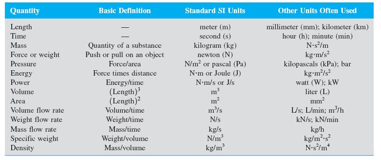
4 SI Units

5 Important Terms Density (): Mass per unit volume of a substance. kg/m 3 in SI units Slug/ft 3 in FPS system of units Specific weight (): Weight per unit volume of substance. N/m 3 in SI units lbs/ft 3 in FPS units m V w V Density and Specific Weight of a fluid are related as: g Where g is the gravitational constant having value 9.8m/s 2 or 32.2 ft/s 2.

6 Important Terms Specific Volume (v): Volume occupied by unit mass of fluid. It is commonly applied to gases, and is usually expressed in cubic feet per slug (m 3 /kg in SI units). Specific volume is the reciprocal of density. SpecificVo lume v 1/

7 Important Terms Specific gravity: It can be defined in either of two ways: a. Specific gravity is the ratio of the density of a substance to the density of water at 4 C. b. Specific gravity is the ratio of the specific weight of a substance to the specific weight of water at 4 C. s liquid l w l w

8 Example The specific wt. of water at ordinary temperature and pressure is 62.4lb/ft 3. The specific gravity of mercury is Compute density of water, Specific wt. of mercury, and density of mercury. Solution: water mercury mercury s s water mercury mercury / g 62.4/ slugs/ft water water 13.56x lb/ ft 13.56x slugs / 3 3 ft 3 (Where Slug = lb.sec2/ ft)

9 Example A certain gas weighs 16.0 N/m 3 at a certain temperature and pressure. What are the values of its density, specific volume, and specific gravity relative to air weighing 12.0 N/m 3 Solution: 1. Density ρ γ /g ρ 16/ kg/m 3 2. Specific u volume υ 1/ρ 3 1/ m /kg 3. Specific gravity s 16/12 s γ f /γ air

10 Example The specific weight of glycerin is 78.6 lb/ft 3. compute its density and specific gravity. What is its specific weight in kn/m 3 Solution: 1. Density / g 2.Specific gravity s s 78.6/ Specific 78.6/ slugs/ft l so 1.260x1000kg/m weight in kn/m / x g 3 w 1260 Kg/m 9.81x kn/m

11 Example Calculate the specific weight, density, specific volume and specific gravity of 1litre of petrol weights 7 N. Solution: Given Volume = 1 litre = 10-3 m 3 Weight = 7 N 1. Specific weight, w = Weight of Liquid/volume of Liquid w = 7/ 10-3 = 7000 N/m 3 2. Density, = /g = 7000/9.81 = kg/m 3

12 Solution (Cont.): 3. Specific Volume = 1/ 1/ =1.4x10-3 m 3 /kg 4. Specific Gravity = s = Specific Weight of Liquid/Specific Weight of Water = Density of Liquid/Density of Water s = /1000 =

13 Example If the specific gravity of petrol is 0.70.Calculate its Density, Specific Volume and Specific Weight. Solution: Given Specific gravity = s = Density of Liquid, s x density of water 2. Specific Volume = 1/ = 0.70x1000 = 700 kg/m 3 1/ x Specific Weight, = 700x9.81 = 6867 N/m 3

14 Compressibility It is defined as: Change in Volume due to change in Pressure. The compressibility of a liquid is inversely proportional to Bulk Modulus (volume modulus of elasticity). Bulk modulus of a substance measures resistance of a substance to uniform compression. dp Where; v is the specific volume and p is the pressure. dp Units: Psi, MPa, As v/dv is a dimensionless ratio, the units of E and p are identical. E E v v ( dv / v) v dv

15 Example At a depth of 8km in the ocean the pressure is 81.8Mpa. Assume that the specific weight of sea water at the surface is kn/m 3 and that the average volume modulus is 2.34 x 10 3 N/m 3 for that pressure range. (a) What will be the change in specific volume between that at the surface and at that depth? (b) What will be the specific volume at that depth? (c) What will be the specific weight at that depth?

16 Solution: / / / ) ( / v v v ) ( / -34.1x10 ) 10 0) /( (81.8 / /10050 / 1/ v ) ( m N v g c kg m b kg m x x v kg m g p a v v v E p p v v v E p v dv v v p E Us ) / ( Equation : ing

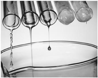
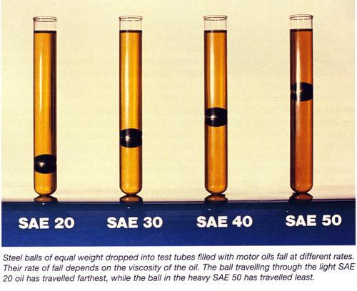
17 Viscosity Viscosity is a measure of the resistance of a fluid to deform under shear stress. It is commonly perceived as thickness, or resistance to flow. Viscosity describes a fluid's internal resistance to flow and may be thought of as a measure of fluid friction. Thus, water is "thin", having a lower viscosity, while vegetable oil is "thick" having a higher viscosity. The friction forces in flowing fluid result from the cohesion and momentum interchange between molecules. All real fluids (except super-fluids) have some resistance to shear stress, but a fluid which has no resistance to shear stress is known as an ideal fluid. It is also known as Absolute Viscosity or Dynamic Viscosity.

18 Viscosity

19 Dynamic Viscosity As a fluid moves, a shear stress is developed in it, the magnitude of which depends on the viscosity of the fluid. Shear stress, denoted by the Greek letter (tau), τ, can be defined as the force required to slide one unit area layer of a substance over another. Thus, τ is a force divided by an area and can be measured in the units of N/m 2 (Pa) or lb/ft 2.

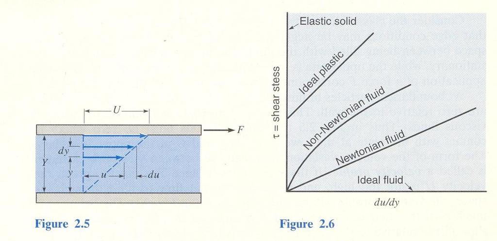
20 Dynamic Viscosity Figure shows the velocity gradient in a moving fluid. U F, U Y Experiments have shown that: Y AU F

21 Dynamic Viscosity The fact that the shear stress in the fluid is directly proportional to the velocity gradient can be stated mathematically as F U du m m A Y dy where the constant of proportionality m (the Greek letter miu) is called the dynamic viscosity of the fluid. The term absolute viscosity is sometimes used.

22 Kinematic Viscosity The kinematic viscosity ν is defined as: Ratio of absolute viscosity to density. m

23 Newtonian Fluid A Newtonian fluid; where stress is directly proportional to rate of strain, and (named for Isaac Newton) is a fluid that flows like water, its stress versus rate of strain curve is linear and passes through the origin. The constant of proportionality is known as the viscosity. A simple equation to describe Newtonian fluid behavior is du m dy Where m = absolute viscosity/dynamic viscosity or simply viscosity = shear stress

24

25 Example Find the kinematic viscosity of liquid in stokes whose specific gravity is 0.85 and dynamic viscosity is poise. Solution: Given S = 0.85 m = poise = x 0.1 Ns/m 2 = 1.5 x 10-3 Ns/m 2 We know that S = density of liquid/density of water density of liquid = S x density of water 0.85 x kg/m 3 Kinematic Viscosity, u m/ 1.5 x 10-3 / x 10-6 m 2 /s = 1.76 x 10-6 x 10 4 cm 2 /s = 1.76 x 10-2 stokes.

26 Example A 1 in wide space between two horizontal plane surface is filled with SAE 30 Western lubricating oil at 80 F. What force is required to drag a very thin plate of 4 sq.ft area through the oil at a velocity of 20 ft/mm if the plate is 0.33 in from one surface.

27 Solution: m 1 2 F F 1 2 F A Force lb.sec/ft 1 2 A U m Y A F 1 F du m dy * * ( From 0.463lb 0.158lb A.1) *(20 / 60) /(0.33/12) lb / *(20 / 60) /(0.67 /12) lb / lb ft ft 2 2

28 Example Assuming a velocity distribution as shown in fig., which is a parabola having its vertex 12 in from the boundary, calculate the shear stress at y= 0, 3, 6, 9 and 12 inches. Fluid s absolute viscosity is 600 P.

29 Solution m 600 P= 600 x 0.1=0.6 N-s/m 2 =0.6 x (1x2.204/9.81 x ) =0.6 x = lb-sec/ft 2 Parabola Equation Y=aX u= a(12-y) 2 u=0 at y=0 so a= 120/12 2= 5/6 u=120-5/6(12-y) 2 =m du/dy du/dy=5/3(12-y) y (in) du/dy

30 Ideal Fluid An ideal fluid may be defined as: A fluid in which there is no friction i.e Zero viscosity. Although such a fluid does not exist in reality, many fluids approximate frictionless flow at sufficient distances, and so their behaviors can often be conveniently analyzed by assuming an ideal fluid.

31 Real Fluid In a real fluid, either liquid or gas, tangential or shearing forces always come into being whenever motion relative to a body takes place, thus giving rise to fluid friction, because these forces oppose the motion of one particle past another. These friction forces give rise to a fluid property called viscosity.

32 Surface Tension Cohesion: Attraction between molecules of same surface It enables a liquid to resist tensile stresses. Adhesion: Attraction between molecules of different surface It enables to adhere to another body. Surface Tension is the property of a liquid, which enables it to resist tensile stress. At the interface between liquid and a gas i.e at the liquid surface, and at the interface between two immiscible (not mixable) liquids, the attraction force between molecules form an imaginary surface film which exerts a tension force in the surface. This liquid property is known as Surface Tension.

33 Surface Tension As a result of surface tension, the liquid surface has a tendency to reduce its surface as small as possible. That is why the water droplets assume a nearly spherical shape. This property of surface tension is utilized in manufacturing of lead shots. Capillary Rise: The phenomenon of rising water in the tube of smaller diameter is called capillary rise.

34 Manometer: Manometer is an improved form of a piezometer tube. With its help we can measure comparatively high pressures and negative pressure also. Following are few types of manometers. 1. Simple Manometer 2. Micro-manometer 3. Differential manometer 4. Inverted differential manometer

35 Simple Manometer: It consists of a tube bent in U-Shape, one end of which is attached to the gauge point and the other is open to the atmosphere. Mercury is used in the bent tube which is 13.6 times heavier than water. Therefore it is suitable for measuring high pressure as well. Procedure: 1. Consider a simple Manometer connected to a pipe containing a light liquid under high pressure. The high pressure in the pipe will force the mercury in the left limb of U-tube to move downward, corresponding the rise of mercury in the right limb.

36 Simple Manometer: 2. The horizontal surface, at which the heavy and light liquid meet in the left limb, is known as datum line. Let h1 = height of light liquid in the left limb above datum. h2 = height of heavy liquid in the right limb above datum. h= Pressure in the pipe, expressed in terms of head of water. s1=sp. Gravity of light liquid. s2=sp. Gravity of heavy liquid. 3. Pressure in left limb above datum = h +s1h1 4. Pressure in right limb above datum = s2h2 5. Since the pressure is both limbs is equal So, h +s1h1 = s2h2 h= (s2h2 - s1h1)

37 Simple Manometer: To measure negative pressure: In this case negative pressure will suck the light liquid which will pull up the mercury in the left limb of U-tube. Correspondingly fall of liquid in the right limb. 6. Pressure in left limb above datum = h +s1h1 + s2h2 7. Pressure in right limb = 0 8. Equating, we get h = -s1h1-s2h2 = -(s1h1+s2h2)

38 Example A simple manometer containing mercury is used to measure the pressure of water flowing in a pipeline. The mercury level in the open tube is 60mm higher than that on the left tube. If the height of water in the left tube is 50mm, determine the pressure in the pipe in terms of head of water. Solution: Pressure head in theleft limb above Z- Z h s h Pressure head in theright limbabove Z- Z 816 mm Equating; h h h 50 mm s h 13.6x mm h (1x50)

39 Example A simple manometer containing mercury was used to find the negative pressure in pipe containing water. The right limb of the manometer was open to atmosphere. Find the negative pressure, below the atmosphere in the pipe.

40 Solution: Pressure head in theleft limbabove Z- Z h s h 1 1 s 2 h 700 mm h 2 h (1x50) (13.6x50) Pressure head in theright limbabove Z- Z 0 Equating; h h -700 mm -7m Gauge pressure in thepipe p h 9.81x(-7) kN/m kPa 68.67kPa (Vacuum) 2

41 Example Figure shows a conical vessel having its outlet at A to which U tube manometer is connected. The reading of the manometer given in figure shows when the vessel is empty. Find the reading of the manometer when the vessel is completely filled with water.

42 Solution: h s mm 0.2m 1 and s 13.6 Let h 1. Let us consider the vessel is to be empty and Z- Z be the datum line. Pressure head in theright limbabove Z- Z s 1 Pressure head in theleft limb above Z- Z 2 1 Equating; 2 2 Pressure head of mercury in terms on head of water. s h h 1xh h 13.6x m h 2.72m

43 2. Consider the vessel to be completely filled with water. As a result, let the mercury level goes down by x meters in the right limb,and themercury level go up by thesame amount in theleft limb. Therefore total height of water in theright limb x h 3 x x 5.72 Pressure head in theright limb1(x 5.72) x 5.72 Weknow that manometer reading in thiscase : 0.2 2x Pressure head in theleft limb 13.6(0.2 2x) x Equating the pressures : x x x 0.115m and manometer reading 0.2 (2x0.115) 0.43m 430 mm

44 Differential Manometer: It is a device used for measuring the difference of pressures, between the two points in a pipe, on in two different pipes. It consists of U-tube containing a heavy liquid (mercury) whose ends are connected to the points, for which the pressure is to be found out. Procedure: Let us take the horizontal surface Z-Z, at which heavy liquid and light liquid meet in the left limb, as datum line. Let, h=difference of levels (also known as differential manomter reading) ha, hb= Pressure head in pipe A and B, respectively. s1, s2= Sp. Gravity of light and heavy liquid respectively.

45 Differential Manometer: 1. Consider figure (a): 2. Pressure head in the left limb above Z-Z = ha+s1(h+h)= ha+s1h+s1h 3. Pressure head in the right limb above Z-Z = hb+s1h+s2h 4. Equating we get, ha+s1h+s1h = hb+s1h+s2h ha-hb=s2h-s1h = h(s2-s1)

46 Differential Manometer: Two pipes at different levels: 1. Pressure head in the left limb above Z-Z = ha+s1h1 2. Pressure head in the right limb above Z-Z = s2h2+s3h3+hb 3. Equating we get, Where; ha+s1h1 = s2h2+s3h3+hb h1= Height of liquid in left limb h2= Difference of levels of the heavy liquid in the right and left limb (reading of differential manometer). h3= Height of liquid in right limb s1,s2,s3 = Sp. Gravity of left pipe liquid, heavy liquid, right pipe liquid, respectively.

47 Example A U-tube differential manometer connects two pressure pipes A and B. The pipe A contains carbon Tetrachloride having a Sp. Gravity 1.6 under a pressure of 120 kpa. The pipe B contains oil of Sp. Gravity 0.8 under a pressure of 200 kpa. The pipe A lies 2.5m above pipe B. Find the difference of pressures measured by mercury as fluid filling U- tube. Solution: Given :s h Let h Differnce Weknow that pressure p Pressure mercury in terms of a 1 a 1.6, p head a of m 9.81 in pipe B, 120kPa; s 2.5m and s 13.6 pressure head p b b measured head of in pipe A, 0.8, p b by water. 20.4m 200kPa;

48 Wealso know that pressure head in Pipe A above 12.2 (s. h ) s. h 12.2 (1.6 x 2.5) 13.6 x h h Pressure head in Pipe B above Z- Z 20.4 s b a h 20.4 (0.8 x h) Equating; h 20.4 (0.8 x h) h m 328 mm 1 Z- Z

49 Inverted Differential Manometer: Type of differential manometer in which an inverted U-tube is used. Used for measuring difference of low pressure. 1. Pressure head in the left limb above Z-Z = ha-s1h1 2. Pressure head in the right limb above Z-Z = hb-s2h2-s3h3 3. Equating we get, ha-s1h1 = hb-s2h2-s3h3 (Where; ha, hb are Pressure in pipes A and B expressed in terms of head of liquid, respectively)

50 UNIT - II FLUID KINEMATICS AND DYNAMICS

51 Fluid Kinematics c c Branch of fluid mechanics which deals with response of fluids in motion without considering forces and energies in them. The study of kinematics is often referred to as the geometry of motion. Flow around cylindrical object CAR surface pressure contours and streamlines

52 Types of Flow c c c c c Ideal and Real flow Incompressible and compressible Laminar and turbulent flows Steady and unsteady flow Uniform and Non-uniform flow

53 Ideal and Real flow c Real fluid flows implies friction effects. Ideal fluid flow is hypothetical; it assumes no friction. Velocity distribution of pipe flow

54 Compressible and incompressible flows c Incompressible fluid flows assumes the fluid have constant density while in compressible fluid flows density is variable and becomes function of temperature and pressure. P 1 P 2 P 1 P 2 v 1 v 2 v 1 v2 v 2 Incompressible fluid Compressible fluid

55 Laminar and turbulent flow c The flow in laminations (layers) is termed as laminar flow while the case when fluid flow layers intermix with each other is termed as turbulent flow. Laminar flow Turbulent flow 5 5 c Reynold s number is used to differentiate between laminar and turbulent flows. Transition of flow from Laminar to turbulent

56 Steady and Unsteady flows Steady flow: It is the flow in which conditions of flow remains constant w.r.t. time at a particular section but the condition may be different at different sections. Flow conditions: velocity, pressure, density or cross-sectional area etc. e.g., A constant discharge through a pipe. Longitudinal Section V t V 0; V contt X X Unsteady flow: It is the flow in which conditions of flow changes w.r.t. time at a particular section. e.g.,a variable discharge through a pipe V t 0; V variable

57 Uniform and Non-uniform flow X c c Uniform flow: It is the flow in which conditions of flow remains constant from section to section. e.g., Constant discharge though a constant diameter pipe V Longitudinal Section V 0; V contt x X c c Non-uniform flow: It is the flow in which conditions of flow does not remain constant from section to section. e.g., Constant discharge through variable diameter pipe 5 7 V X Longitudinal Section V 0; V variable x

58 One, Two and Three Dimensional Flows c Although in general all fluids flow three-dimensionally, with pressures and velocities and other flow properties varying in all directions, in many cases the greatest changes only occur in two directions or even only in one. In these cases changes in the other direction can be effectively ignored making analysis much more simple. c Flow is one dimensional if the flow parameters (such as velocity, pressure, depth etc.) at a given instant in time only vary in the direction of flow and not across the cross-section Water surface Mean velocity Longitudinal section of rectangular channel Cross-section Velocity profile

59 One, Two and Three Dimensional Flows c Flow is two-dimensional if it can be assumed that the flow parameters vary in the direction of flow and in one direction at right angles to this direction Two-dimensional flow over a weir c Flow is three-dimensional if the flow parameters vary in all three directions of flow Three-dimensional flow in stilling basin

60 Path line and stream line c c Pathline: It is trace made by single particle over a period of time. Streamline show the mean direction of a number of particles at the same instance of time. c Character of Streamline c 1. Streamlines can not cross each other. (otherwise, the cross point will have two tangential lines.) c 2. Streamline can't be a folding line, but a smooth curve. c 3. Streamline cluster density reflects the magnitude of velocity. (Dense streamlines mean large velocity; while sparse streamlines mean small velocity. ) Flow around cylindrical object

61 Streakline and streamtubes c c A Streakline is the locus of fluid particles that have passed sequentially through a prescribed point in the flow. It is an instantaneous picture of the position of all particles in flow that have passed through a given point. c c Streamtube is an imaginary tube whose boundary consists of streamlines. The volume flow rate must be the same for all cross sections of the stream tube.

62 Continuity c Matter cannot be created or destroyed - (it is simply changed in to a different form of matter). c This principle is know as the conservation of mass and we use it in the analysis of flowing fluids. c The principle is applied to fixed volumes, known as control volumes shown in figure: An arbitrarily shaped control volume. For any control volume the principle of conservation of mass says Mass entering per unit time -Mass leaving per unit time = Increase of mass in the control volume per unit time

63 Continuity Equation c For steady flow there is no increase in the mass within the control volume, so Mass entering per unit time = Mass leaving per unit time c c Derivation: Lets consider a stream tube. c ρ 1, v 1 and A 1 are mass density, velocity and cross-sectional area at section 1. Similarly, ρ 2, v 2 and A 2 are mass density, velocity and crosssectional area at section 2. c According to mass conservation dm CV M 1 M 2 dt dm 1 A 1 V 1 2 A 2 V 2 CV dt A stream tube M 1 1 A 1 V 1 M 2 2 A 2 V 2

64 Continuity Equation c For steady flow condition dm CV / dt 0 c Similarly 1 A 1 V 1 2 A 2 V A 1 V 1 2 A 2 V 2 M 1 A 1 V 1 2 A 2 V 2 c Hence, for stead flow condition, mass flow rate at section 1= mass flow rate at section 2. i.e., mass flow rate is G constant. 1 ga 1 V 1 2 ga 2 V 2 c Assuming incompressible fluid, 1 2 A 1 V 1 A 2 V 2 Q 1 Q 2 Q 1 Q 2 Q 3 Q 4 c Therefore, according to mass conservation for steady flow of incompressible fluids volume flow rate remains same from section to section.

65 EQUATION FOR STEADY MOTION OF AN IDEAL FLUID ALONG A STREAMLINE, AND BERNOULLI'S THEOREM Referring to Fig., let us consider frictionless steady flow of an ideal fluid along the streamline. We shall consider the forces acting in the direction of the streamline on a small element of the fluid in the stream tube, and we shall apply Newton's second law, that is F = ma. The cross-sectional area of the element at right angles to the streamline may have any shape and varies from A to A + da. Recalling that in steady flow the velocity does not vary at a point (local acceleration = 0), but that it may vary with position (convective acceleration 0).

66 Bernoulli's Theorem: The mass of the fluid element is m = ds(a + 1/2dA) = dsa when we neglect second order terms. The forces tending to accelerate or decelerate this mass along s are: (a) the pressure forces: 1 pa p dpda ( p dp)( A da) 2 dpa (b) the weight component in the direction of motion: A 1 2 da cos dz pgdsa ds pgadz Applying ƐF = ma along the streamline, we get, dpa pgadz ( pdsa) a

67 Bernoulli's Theorem: Dividing by the volume dsa, dp ds pg dz ds This states that the pressure gradient along the streamline combined with the weight component in that direction causes the acceleration a of the element. Recalling that a = V(dV/ds) for steady flow (Equation 4.24), we get: dp ds pg dz ds pv pa dv ds Multiplying by ds/p and rearranging, dp p gdz VdV 0 (5.5)

68 Bernoulli's Theorem: We commonly refer to this equation as the one-dimensional Euler 3 equation, because Leonhard Euler ( ), a Swiss mathematician, first derived it in about It applies to both compressible and incompressible flow, since the variation of p over the elemental length ds is small. Dividing through by g, we can also express Eq. (5.5) as: dp dz d V 2 2g 0 (5.6)

69 Assumptions: 1. It assumes viscous (friction) effects are negligible 2. It assumes the flow is steady 3. The equation applies along a streamline 4. It assumes the fluid to be incompressible 5. It assumes no energy is added to or removed from the fluid along the streamline

70 Problem: Glycerin (specific gravity 1.26) in a processing plant flows in a pipe at a rate of 700 L/s. At a point where the pipe diameter is 600 mm, the pressure is 300 kpa. Find the pressure at a second point where the pipe diameter is 300 mm if the second point is 1.0 m lower than the first point, neglect the head loss.

71 Solution:

72 The force due the flow around a pipe bend Consider a pipe bend with a constant cross section lying in the horizontal plane and turning through an angle of θ

73 Because the fluid changes direction, a force (very large in the case of water supply pipes,) will act in the bend. If the bend is not fixed it will move and eventually break at the joints. We need to know how much force a support (thrust block) must withstand. Step in Analysis: 1. Draw a control volume 2. Decide on co-ordinate axis system 3. Calculate the total force (rate of change of momentum) 4. Calculate the pressure force 5. Calculate the body force 6. Calculate the resultant force

74 The control volume is draw in the above figure, with faces at the inlet and outlet of the bend and encompassing the pipe walls. It is convenient to choose the co-ordinate axis so that one is pointing in the direction of the inlet velocity. In the above figure the x-axis points in the direction of the inlet velocity.

75 Calculate the total force: In the x-direction: In the y-direction: ) cos ( cos ) ( u Q u F u u u u u Q u F tx x x x x tx sin sin 0 sin 0 ) ( Qu F u u u u u Q u F ty y y y y ty

76 Calculate the pressure force F p = pressure force at 1 - pressure force at 2 F px = p 1 A 1 cos 0 p 2 A 2 cos θ = p 1 A 1 p 2 A 2 cos θ F py = p 1 A 1 sin 0 p 2 A 2 sin θ = p 2 A 2 sin θ Calculate the body force There are no body forces in the x or y directions. The only body force is that exerted by gravity (which acts into the paper in this example - a direction we do not need to consider). F bx = F by = 0

77 Calculate the resultant force F Rx = F tx - F px - F bx F Ry = F ty - F py - F by F Rx F Tx F px 0 Q( u 2 cos u 1 ) p 1 A 1 p 2 A 2 cos F Ry F Ty F py 0 Qu 2 sin p 2 A 2 sin

78 And F resultan t F tan 1 ( F F Ry Rx 2 Rx ) The force on the bend is the same magnitude but in the opposite direction F 2 Ry R = - F resultant

79 UNIT - III BOUNDAR LAYER THEORY AND FLOW THROUGH PIPES

80 Description of Boundary Layer U w : wall shear stresses In the immediate vicinity of the boundary surface, the velocity of the fluid increases gradually from zero at boundary surface to the velocity of the mainstream. This region is known as BOUNDARY LAYER. Large velocity gradient leading to appreciable shear stress: u m y y 0 The nominal thickness of BOUNDARY LAYER is defined as the distance from the boundary where the velocity of fluid is 99 % of free stream velocity

81 Description of Boundary Layer U shear stress: u m y w : wall shear stresses Consists of two layers: CLOSE TO BOUNDARY : large velocity gradient, appreciable viscous forces. OUTSIDE BOUNDARY LAYER: viscous forces are negligible, flow may be treated as non-viscous Shear stress or inviscid. acting at the plate surface sets up a shear force which opposes the fluid motion, and fluid close to the wall is decelerated. Theoretical understanding on Boundary layer development is very important to determine the velocity gradient and hence shear forces on the surface.

82 Development of Boundary Layer The boundary layer thickness increases as the distance x from leading edge is increases. This is because of viscous forces that dissipate more and more energy of fluid stream as the flow proceeds and large group of particles are slow downed. In laminar boundary layer the particles are moving along stream lines. The disturbance in fluid flow in boundary layer is amplified and the flow become unstable and the fluid flow undergoes transition from laminar to turbulent flow. This regime is called transition regime.

83 Development of Boundary Layer After going through transition zone of finite length the flow becomes completely turbulent which is characterized by three dimensional, random motion of fluctuation induced bulk motion parcel of fluid. LAMINAR BOUNDARY LAYER PROFILE PARABOLIC TURBULENT BOUNDARY LAYER PROFILE BECOMES LOGARITHMIC

84 Development of Boundary Layer BL depends on Reynold s number & also on the surface roughness. Roughness of the surface adds to the disturbance in the flow & hastens the transition from laminar to turbulent. For laminar flow For Turbulent flow u m y u m y Where ε is the eddy viscosity and is often much larger than µ.

85 Boundary Layer Thickness for Laminar and Turbulent The boundary layer thickness is governed by parameters like incoming velocity, kinematic viscosity of fluid etc. lam For laminar flow 5.0x Pohlhausen (Exact solution) Re For Turbulent flow x 0.377x tur Re 1 5 lam 5.835x Blassius Re x (Approximate solution)

86 Flow Patterns and Regimes within Laminar and Turbulent Boundary Layer As mentioned above, very close to the plane surface the flow remains laminar and a linear velocity profile may be assumed. In this region, the velocity gradient is governed by the fluid viscosity u y m

87 Flow Patterns and Regimes within Laminar and Turbulent Boundary Layer In turbulent flow, owing to the random motion of the fluid particles, eddy patterns are set up in the boundary layer which sweep small masses of fluid up and down through the boundary layer, moving in a direction perpendicular to the surface and the mean flow direction.

88 Flow Patterns and Regimes within Laminar and Turbulent Boundary Layer Conversely, slow-moving fluid is lifted into the upper levels, slowing down the fluid stream and, by doing so, effectively thickening the boundary layer, explaining the more rapid growth of the turbulent boundary layer compared with the laminar one. Owing to these eddies, fluid from the upper higher-velocity areas is forced into the slower-moving stream above the laminar sublayer, having the effect of increasing the local velocity here relative to its value in the laminar sublayer. In order to explain this process, the eddy viscosity, ε should be added in Shear stress formulation. m u y

89 Effect of Pressure Gradient On Boundary Layer Development The presence of a pressure gradient p/ x effectively means a u/ x term, i.e. the flow stream velocity changes across the surface. for example, consider a curved surface, then the velocity variation can be shown as:

90 Effect of Pressure Gradient on Boundary Layer Development If the pressure decreases in the downstream direction, then the boundary layer tends to be reduced in thickness, and this case is termed a favorable pressure gradient. If the pressure increases in the downstream direction, then the boundary layer thickens rapidly; this case is referred to as an adverse pressure gradient.

91 A conduit is any pipe, tube, or duct that is completely filled with a flowing fluid. Examples include a pipeline transporting liquefied natural gas, a microchannel transporting hydrogen in a fuel cell, and a duct transporting air for heating of a building. A pipe that is partially filled with a flowing fluid, for example a drainage pipe, is classified as an open-channel flow. The main goal of this chapter is to describe how to predict head loss. Predicting head loss involves classifying flow as laminar or turbulent and then using equations to calculate head losses in pipes and components.

92 10.1 Classifying Flow The flow in a conduit may be classified as: (a) whether the flow is laminar or turbulent, and (b) whether the flow is developing or fully developed. Laminar Flow and Turbulent Flow Flow in a conduit is classified as being either laminar or turbulent, depending on the magnitude of the Reynolds number. The original research involved visualizing flow in a glass tube as shown in Fig. 10.1a. Reynolds 1 in the 1880s injected dye into the center of the tube and observed the following: - When the velocity was low, the streak of dye flowed down the tube with little expansion, as shown in Fig. 10.1b. However, if the water in the tank was disturbed, the streak would shift about in the tube. - If velocity was increased, at some point in the tube, the dye would all at once mix with the water as shown in Fig. 10.1c. - When the dye exhibited rapid mixing (Fig. 10.1c), illumination with an electric spark revealed eddies in the mixed fluid as shown in Fig. 10.1d.

93 Figure 10.1 Reynolds' experiment. (a) Apparatus. (b) Laminar flow of dye in tube. (c) Turbulent flow of dye in tube. (d) Eddies in turbulent flow.

94 Reynolds showed that the onset of turbulence was related to a π-group that is now called the Reynolds number (Re = ρvd/μ) in honor of Reynolds' pioneering work. Reynolds discovered that if the fluid in the upstream reservoir was not completely still or if the pipe had some vibrations, then the change from laminar to turbulent flow occurred at Re ~ However, if conditions were ideal, it was possible to reach a much higher Reynolds number before the flow became turbulent. Reynolds also found that, when going from high velocity to low velocity, the change back to laminar flow occurred at Re ~ Based on Reynolds' experiments, engineers use guidelines to establish whether or not flow in a conduit will be laminar or turbulent. The (10.1) guidelines used in this text are as follows:

95 The range (2000 Re 3000) corresponds to a the type of flow that is unpredictable because it can changes back and forth between laminar and turbulent states. Recognize that precise values of Reynolds number versus flow regime do not exist. Thus, the guidelines given in Eq. (10.1) are approximate and other references may give slightly different values. For example, some references use Re = 2300 as the criteria for turbulence. There are several equations for calculating Reynolds number in a pipe

96 Derivation of the Darcy-Weisbach Equation To derive the Darcy-Weisbach equation, consider Fig Assume fully developed and steady flow in a round tube of constant diameter D. Situate a cylindrical control volume of diameter D and length L inside the pipe. Define a coordinate system with an axial coordinate in the streamwise direction (s direction) and a radial coordinate in the r direction.

97 (10.5) The net efflux of momentum is zero because the velocity distribution at section 2 is identical to the velocity distribution at section 1. The momentum accumulation term is also zero because the flow is steady. Thus, Eq. (10.5) simplifies to ΣF = 0. Forces are shown in Fig Summing forces in the streamwise direction gives Since, sin = (z/l), the equation becomes, Figure 10.5 Force diagram.

98 Next, apply the energy equation to the control volume shown in Fig Recognize that h p = h t = 0, V 1 = V 2, and α1 = α2. Thus, the energy equation reduces to Combine the equation from the momentum and the above (form the energy) and replace L by L. Also, introduce a new symbol h f to represent head loss in pipe. Rearrange the right side of Eq. (10.9).

99 Define a new π-group called the friction factor f that gives the ratio of wall shear stress ( o ) to kinetic pressure (ρv 2 /2): In the technical literature, the friction factor is identified by several different labels that are synonymous: friction factor, Darcy friction factor, Darcy-Weisbach friction factor, and the resistance coefficient. There is also another coefficient called the Fanning friction factor, often used by chemical engineers, which is related to the Darcy-Weisbach friction factor by a factor of 4. This text uses only the Darcy-Weisbach friction factor. Combining the previous equations, gives the Darcy-Weisbach equation:

100 To use the Darcy-Weisbach equation, the flow should be fully developed and steady. The Darcy-Weisbach equation is used for either laminar flow or turbulent flow and for either round pipes or nonround conduits such as a rectangular duct. The Darcy-Weisbach equation shows that head loss depends on the friction factor, the pipe-length-to-diameter ratio, and the mean velocity squared. The key to using the Darcy-Weisbach equation is calculating a value of the friction factor f.

101 Moody Diagram

102 Minor Losses In addition to head loss due to friction, there are always other head losses due to pipe expansions and contractions, bends, valves, and other pipe fittings. These losses are usually known as minor losses (h Lm ). In case of a long pipeline, the minor losses maybe negligible compared to the friction losses, however, in the case of short pipelines, their contribution may be significant.

103 Losses due to pipe fittings where h Lm K V 2 2g h Lm = minor loss K = minor loss coefficient V = mean flow velocity Type K Exit (pipe to tank) 1.0 Entrance (tank to pipe) elbow elbow 0.4 T-junction 1.8 Gate valve Typical K values

104 Sudden Enlargement As fluid flows from a smaller pipe into a larger pipe through sudden enlargement, its velocity abruptly decreases; causing turbulence that generates an energy loss. The amount of turbulence, and therefore the amount of energy, is dependent on the ratio of the sizes of the two pipes. The minor loss (h Lm )is calculated from; h Lm K E V 2 a 2g (4.16a) where is K E is the coefficient of expansion, and the values depends on the ratio of the pipe diameters (D a /D b ) as shown below. D a /D b K Values of K E vs. D a /D b

105 Flow at Sudden Enlargement

106 Sudden Contraction The energy loss due to a sudden contraction can be calculated using the following; 2 Vb hlm KC 2g (4.16b) The K C is the coefficient of contraction and the values depends on the ratio of the pipe diameter (D b /D a ) as shown below. D b /D a K Values of K C vs. D b /D a Flow at sudden contraction

107 Example Water at 10C is flowing at a rate of 0.03 m3/s through a pipe. The pipe has 150-mm diameter, 500 m long, and the surface roughness is estimated at 0.06 mm. Find the head loss and the pressure drop throughout the length of the pipe. Solution: From Table 1.3 (for water): = 1000 kg/m 3 and m =1.30x10-3 N.s/m 2 V = Q/A and A=R 2 A = (0.15/2) 2 = m 2 V = Q/A =0.03/ =1.7 m/s Re = (1000x1.7x0.15)/(1.30x10-3 ) = 1.96x105 > 2000 turbulent flow To find, use Moody Diagram with Re and relative roughness (k/d). k/d = 0.06x10-3 /0.15 = 4x10-4 From Moody diagram, The head loss may be computed using the Darcy-Weisbach equation. h f L D 2 V 2g 500 x x 8.84m x 2 x The pressure drop along the pipe can be calculated using the relationship: ΔP=gh f = 1000 x 9.81 x 8.84 ΔP = 8.67 x 104 Pa

108 UNIT - IV TURBO MACHINERY

109 Force exerted by the jet on a stationary plate Impact of Jets The jet is a stream of liquid comes out from nozzle with a high velocity under constant pressure. When the jet impinges on plates or vanes, its momentum is changed and a hydrodynamic force is exerted. Vane is a flat or curved plate fixed to the rim of the wheel 1. Force exerted by the jet on a stationary plate a) Plate is vertical to the jet b) Plate is inclined to the jet c) Plate is curved 2. Force exerted by the jet on a moving plate a) Plate is vertical to the jet b) Plate is inclined to the jet c) Plate is curved

110 Impulse-Momentum Principle From Newton's 2 nd Law: F = m a = m (V 1 - V 2 ) / t Impulse of a force is given by the change in momentum caused by the force on the body. Ft = mv 1 mv 2 = Initial Momentum Final Momentum Force exerted by jet on the plate in the direction of jet, F = m (V 1 V 2 ) / t = (Mass / Time) (Initial Velocity Final Velocity) = (ρq) (V 1 V 2 ) = (ρav) (V 1 V 2 )

111 Force exerted by the jet on a stationary plate Plate is vertical to the jet F = av 2 If Plate is moving at a velocity of U m/s, F = a(v-u) 2

112 Problems: 1. A jet of water 50 mm diameter strikes a flat plate held normal to the direction of jet. Estimate the force exerted and work done by the jet if a. The plate is stationary b. The plate is moving with a velocity of 1 m/s away from the jet along the line of jet. The discharge through the nozzle is 76 lps. 2. A jet of water 50 mm diameter exerts a force of 3 kn on a flat vane held perpendicular to the direction of jet. Find the mass flow rate.

113 Force exerted by the jet on a stationary plate Plate is inclined to the jet F N = av 2 sin F x = F N sin F x = F N cos

114 Force exerted by the jet on a moving plate Plate is inclined to the jet F N = a(v-u) 2 sin F x = F N sin F x = F N cos

115 Problems: 1. A jet of data 75 mm diameter has a velocity of 30 m/s. It strikes a flat plate inclined at 45 0 to the axis of jet. Find the force on the plate when. a. The plate is stationary b. The plate is moving with a velocity of 15 m/s along and away from the jet. Also find power and efficiency in case (b) 2. A 75 mm diameter jet having a velocity of 12 m/s impinges a smooth flat plate, the normal of which is inclined at 60 0 to the axis of jet. Find the impact of jet on the plate at right angles to the plate when the plate is stationery. a. What will be the impact if the plate moves with a velocity of 6 m/s in the direction of jet and away from it. b. What will be the force if the plate moves towards the plate.

116 Force exerted by the jet on a stationary plate Plate is Curved and Jet strikes at Centre F = av 2 (1+ cos )

117 Force exerted by the jet on a moving plate Plate is Curved and Jet strikes at Centre F = a(v-u) 2 (1+ cos )

118 Problems: 1. A jet of water of diameter 50 mm strikes a stationary, symmetrical curved plate with a velocity of 40 m/s. Find the force extended by the jet at the centre of plate along its axis if the jet is deflected through at the outlet of the curved plate 2. A jet of water from a nozzle is deflected through 60 0 from its direction by a curved plate to which water enters tangentially without shock with a velocity of 30m/s and leaver with a velocity of 25 m/s. If the discharge from the nozzle is 0.8 kg/s, calculate the magnitude and direction of resultant force on the vane.

119 Force exerted by the jet on a stationary plate (Symmetrical Plate) Plate is Curved and Jet strikes at tip F x = 2aV 2 cos

120 Force exerted by the jet on a stationary plate (Unsymmetrical Plate) Plate is Curved and Jet strikes at tip F x = av 2 (cos + cos )

121 Problems: 1. A jet of water strikes a stationery curved plate tangentially at one end at an angle of The jet of 75 mm diameter has a velocity of 30 m/s. The jet leaves at the other end at angle of 20 0 to the horizontal. Determine the magnitude of force exerted along x and y directions.

122 Force exerted by the jet on a moving plate Considering Relative Velocity, If < 90 0 F x = av r1 (V r1 cos + V r2 cos ) OR F x = av r1 (V W1 + V W2 )

123 Force exerted by the jet on a moving plate Considering Relative Velocity, If = 90 0 F x = av r1 (V r1 cos V r2 cos ) OR F x = av r1 (V W1 )

124 Force exerted by the jet on a moving plate Considering Relative Velocity, If = 90 0 F x = av r1 (V r1 cos V r2 cos ) OR F x = av r1 (V W1 V W2 )

125 Impact of jet on a series of flat vanes mounted radially on the periphery of a circular wheel F = av (V-U)

126 Impact of jet on a series of flat vanes mounted radially on the periphery of a circular wheel F = av (V-U) (1+ cos )

127 Problems: 1. A jet of water of diameter 75 mm strikes a curved plate at its centre with a velocity of 25 m/s. The curved plate is moving with a velocity of 10 m/s along the direction of jet. If the jet gets deflected through in the smooth vane, compute. a) Force exerted by the jet. b) Power of jet. c) Efficiency of jet. 2. A jet of water impinges a curved plate with a velocity of 20 m/s making an angle of 20 0 with the direction of motion of vane at inlet and leaves at to the direction of motion at outlet. The vane is moving with a velocity of 10 m/s. Compute. i) Vane angles, so that water enters and leaves without shock. ii) Work done per unit mass flow rate

128 Force exerted by the jet on a moving plate (PELTON WHEEL) Considering Relative Velocity, F x = av r1 (V r1 V r2 cos ) OR F x = av r1 (V W1 V W2 ) Work done / sec = F.U Power = F. U Efficiency = F.U ½ mv 2

129 Force exerted by the jet on a moving plate (PELTON WHEEL) Considering Relative Velocity, F x = av r1 (V r1 V r2 cos ) OR F x = av r1 (V W1 V W2 ) Work done / sec = F.U Power = F. U Efficiency = F.U ½ mv 2

130 Hydraulic machinery Turbine is a device that extracts energy from a fluid (converts the energy held by the fluid to mechanical energy) Pumps are devices that add energy to the fluid (e.g. pumps, fans, blowers and compressors).

131 Turbines Hydro electric power is the most remarkable development pertaining to the exploitation of water resources throughout the world Hydroelectric power is developed by hydraulic turbines which are hydraulic machines. Turbines convert hydraulic energy or hydropotential into mechanical energy. Mechanical energy developed by turbines is used to run electric generators coupled to the shaft of turbines

132 Types of turbines Turbines can be classified on the basis of: Head and quantity of water available Hydraulic action of water Direction of flow of water in the runner Specific speed of turbines Disposition of the shaft of the runner

133 Classification of turbines Based on head and quantity of water According to head and quantity of water available, the turbines can be classified into a) High head turbines b) Medium head turbines c) Low head turbines a) High head turbines High head turbines are the turbines which work under heads more than 250m. The quantity of water needed in case of high head turbines is usually small. The Pelton turbines are the usual choice for high heads.

134 Classification of turbines Based on head and quantity of water b) Medium head turbines The turbines that work under a head of 45m to 250m are called medium head turbines. It requires medium flow of water. Francis turbines are used for medium heads. c) Low head turbines Turbines which work under a head of less than 45m are called low head turbines. Owing to low head, large quantity of water is required. Kaplan turbines are used for low heads.

135 Classification of turbines Based on hydraulic action of water According to hydraulic action of water, turbines can be classified into a) Impulse turbines b) Reaction turbines a) Impulse turbines If the runner of a turbine rotates by the impact or impulse action of water, it is an impulse turbine. b) Reaction turbines These turbines work due to reaction of the pressure difference between the inlet and the outlet of the runner.

136 Classification of turbines Based on direction of flow of water in the runner Depending upon the direction of flow through the runner, following types of turbines are there a) Tangential flow turbines b) Radial flow turbines c) Axial flow turbines d) Mixed flow turbines a) Tangential flow turbines When the flow is tangential to the wheel circle, it is a tangential flow turbine. A Pelton turbine is a Tangential flow turbine.

137 Classification of turbines Based on direction of flow of water in the runner b) Radial flow turbines In a radial flow, the path of the flow of water remains in the radial direction and in a plane normal to the runner shaft. No pure radial flow turbine is in use these days. c) Axial flow turbines When the path of flow water remains parallel to the axis of the shaft, it is an axial flow turbine. The Kaplan turbine is axial flow turbine d) Mixed flow turbines When there is gradual change of flow from radial to axial in the runner, the flow is called mixed flow. The Francis turbine is a mixed flow turbine.

138 Classification of turbines Based on specific speed of turbines Specific speed of a turbine is defined as the speed of a geometrically similar turbine which produces a unit power when working under a unit head. The specific speed of Pelton turbine ranges between 8-30, Francis turbines have specific speed between , Specific speed of Kaplan lies between Based on disposition of shaft of runner Usually, Pelton turbines are setup with horizontal shafts, where as other types have vertical shafts.

139 Main dimensions for the Pelton runner

140 The ideal Pelton runner u Absolute velocity from nozzle: c c1 2g c1 1 2g H 1 H n Circumferential speed: c 1 u u 1 2g Hn Euler`s turbine equation: n h 2(u1 c1u u2 c2u) c u 1 1 c u2 0 h 2 2 ( u1 c1 u u2 c u) 2(0, ,5 0) 1

141 The real Pelton runner For a real Pelton runner there will always be losses. We will therefore set the hydraulic efficiency to: h 0.96 The absolute velocity from the nozzle will be: 0.99 c u C 1u can be set to 1,0 when dimensioning the turbine. This gives us: h 2(u1 c1u u2 c2u) u n 2c 1u 0,96 21,0 1 0,48

142 Runner diameter Rules of thumb: D = 10 d s D = 15 d s H n < 500 m H n = 1300 m D < 9,5 d s because water D > 15 d s Pelton must be avoided will be lost is for very high head

143 Speed number Qz 0,5 u 1,0 c 1 1u 4 d c 4 d Q 2 s 1u 2 s D 1 H g 2 D H g 2 H g 2 D u 2 H g 2 n n n 1 n 4 z D d s 4 z d D 1 z Q 2 s

144 Francis turbines The water enters the turbine through the outer periphery of the runner in the radial direction and leaves the runner in the axial direction, and hence it is called mixed flow turbine. It is a reaction turbine and therefore only a part of the available head is converted into the velocity head before water enters the runner. The pressure head goes on decreasing as the water flows over the runner blades. The static pressure at the runner exit may be less than the atmospheric pressure and as such, water fills all the passages of the runner blades. The change in pressure while water is gliding over the blades is called reaction pressure and is partly responsible for the rotation of the runner. A Francis turbine is suitable for medium heads (45 to 400 m) and requires a relatively large quantity of water.

145 Variations of Francis

146 Variations of Francis

147 Parts of A Francis Turbine

148 Hydraulic efficiency of Francis Hydraulic System g V h g V h Losses hydraulic g V h g V h hydraulic

149 Spiral Casing Spiral Casing : The fluid enters from the penstock to a spiral casing which completely surrounds the runner. This casing is known as scroll casing or volute. The cross-sectional area of this casing decreases uniformly along the circumference to keep the fluid velocity constant in magnitude along its path towards the stay vane/guide vane.

150 UNIT - V CENTRIFUGAL AND RECIPROCATING PUMPS

151 Types of Pumps Positive displacement piston pump Diaphragm pump peristaltic pump Rotary pumps gear pump two-lobe rotary pump screw pump Jet pumps Turbomachines axial-flow (propeller pump) radial-flow (centrifugal pump) mixed-flow (both axial and radial flow)

152 Reciprocating action pumps Piston pump can produce very high pressures hydraulic fluid pump high pressure water washers diaphragm pump

153 total flow Positive Displacement Pumps What happens if you close a valve on the effluent side of a positive displacement pump? What does flow rate vs. time look like for a piston pump? st piston 2nd piston 3rd piston 3 pistons revolutions Thirsty Refugees

154 Centrifugal Pumps Centrifugal pumps accelerate a liquid The maximum velocity reached is the velocity of the periphery of the impeller The kinetic energy is converted into potential energy as the fluid leaves the pump The potential energy developed is approximately equal to the velocity head at the periphery of the impeller h p = 2 V 2g A given pump with a given impeller diameter and speed will raise a fluid to a certain height regardless of the fluid density

155 Radial Pumps centrifugal also called pumps broad range of applicable flows and heads higher heads can be achieved by increasing the diameteror the rotational speed of the impeller h p 2 V = 2g Discharge Suction Eye Flow Expansion Casing Impeller Impeller Vanes

156 Head-Discharge Curve circulatory flow - inability of finite number of blades to guide flow friction - shock - incorrect angle of blade inlet V 2 other losses bearing friction packing friction disk friction V 2 internal leakage C H = h p w hg p 2 2 D Theoretical head-discharge curve Actual headdischarge curve C Q Q Q 3 D

157 Pump Power Requirements P w =gqh p Water power e e P m P m P w P s P P s m gqh = ee P m p Subscripts w = water p = pump s = shaft m = motor

158 Power (% of design) Impeller Shape vs. Power Curves radial axial S 1 - O Discharge (% of design) Implications

159 Affinity Laws With speed,, held constant: P P p p h h w w æ ö = ç è ø Q Q ä With diameter, D, held constant: P D P D æ ö = ç è ø p p h D h D æ ö = ç è ø Q D Q D æ ö = ç è ø 2 2 p H hg C D w = 3 Q Q C D H Q P 3 D 5 P C P homologous Q C held constant

160 Dimensionless Performance Curves C H hg = w D p D=0.366 m Q C Q shape 1 2 C Q 0.75 D S ä Curves for a particular pump 3 4 CH (defined at max efficiency) ä Independent of the fluid! Efficiency

161 Efficiency Pump Example Given a pump with shape factor of 4.57, a diameter of 366 mm, a 2-m head, a speed of 600 rpm, and dimensionless performance curves (previous slide). What will the discharge be? 0.07 How large a motor will be needed if motor 0.06 C 0.05 H Hg 2 D D=0.366 m 0.01 efficiency is 95%? Q C Q 3 D Exercise

162 Pumps in Parallel or in Series Parallel Flow Head Series Flow Head Multistage adds same same adds

163 Vapor pressure (Pa) Cavitation in Water Pumps water vapor bubbles form when the pressure is less than the vapor pressure of water very high pressures (800 MPa or 115,000 psi) develop when the vapor bubbles collapse Temperature (C)

164 Net Positive Suction Head NPSH R - absolute pressure in excess of vapor pressure required at pump inlet to prevent cavitation given by pump manufacturer determined by the water velocity at the entrance to the pump impeller NPSH A - pressure in excess of vapor pressure available at pump inlet determined by pump installation (elevation above reservoir, frictional losses, water temperature) If NPSH A is less than NPSH R cavitation will occur

165 Net Positive Suction Head 2 Elevation datum 1 z NPSH R p V p = + - g 2g g 2 s s v Absolute pressure s = suction Total head -p v! NPSH R 2 = peye p V v eye g - g + 2g At cavitation! NPSH R increases with Q 2! How much total head in excess of vapor pressure is available?

166 NPSH A 2 2 p1 V1 p2 V2 z1 z2 h g + 2g + = g + 2g patm ps Vs zreservoir h g + = g + 2g + p 2 atm s s - Dz- h p V L = + g g 2g L L p p p V p g g g 2g g 2 atm - D v s s v z - h - = + - L Subtract vapor pressure p g atm p - D - - = g v z hl NPSH A

167 NPSH r Illustrated P v NPSH r Pressure in excess of vapor pressure required to prevent cavitation NPSH r can exceed atmospheric pressure

168 NPSH problem Determine the minimum reservoir level relative to the pump centerline that will be acceptable. The NPSH r for the pump is 2.5 m. Assume you have applied the energy equation and found a head loss of 0.5 m.? 18 C Exercise

169 Pumps in Pipe Systems Pipe diameter is 0.4 m and friction factor is What is the pump discharge? 60 m 1 km p 1 V 2 1 2g z h p 2 1 p V 2 2 2g z h 2 l 1 m h p z 2 z 1 h l h p f(q) often expressed as h = a - bq p 2

170 Head (m) Pumps in Pipe Systems 120 system operating point h p Static head Discharge (m 3 /s) Head vs. discharge curve for pump Could you solve this with a dimensionless performance curve? What happens as the static head changes (a tank fills)? C H hg = w D p 2 2

171 Priming The pressure increase created is proportional to the density of the fluid being pumped. A pump designed for water will be unable to produce much pressure increase when pumping air Density of air at sea level is kg/m 3 Change in pressure produced by pump is about 0.1% of design when pumping air rather than water! C H hg = w D p 2 2 p C H 2 D 2 p C H 2 D 2

172 Priming Solutions Applications with water at less than atmospheric pressure on the suction side of the pump require a method to remove the air from the pump and the inlet piping Solutions foot valve priming tank vacuum source self priming priming tank foot valve to vacuum pump

173 Self-Priming Centrifugal Pumps Require a small volume of liquid in the pump Recirculate this liquid and entrain air from the suction side of the pump The entrained air is separated from the liquid and discharged in the pressure side of the pump