Probabilistic Fundamentals in Robotics
|
|
|
- Raymond McDonald
- 6 years ago
- Views:
Transcription
1 Probabilistic Fundamentals in Robotics Probabilistic Models of Mobile Robots Robot localization Basilio Bona DAUIN Politecnico di Torino June 2011 Course Outline Basic mathematical framework Probabilistic models of mobile robots Mobile robot localization problem Robotic mapping Probabilistic planning and control Reference textbook Thrun, Burgard, Fox, Probabilistic Robotics, MIT Press, robotics.org/ Basilio Bona June
2 Mobile robot localization problem Mobile robot localization: Markov and Gaussian Introduction Markov localization EKF localization Multi hypothesis tracking UKF localization Mobile robot localization: Grid and Monte Carlo Grid localization Monte Carlo localization Localization in dynamic environments Basilio Bona June Introduction Localization or position estimation is the problem of determining the pose of a rover relative to a given map of the environment In other words, localization is the process of establishing the correspondencebet between eenthe mapreference frameandthe and local reference frame of the rover Hence coordinate transformation is necessary: from robot centered local coordinate frame to global reference frame The pose x t =(x y θ) of the robot is not known and cannot be measured directly with a sensor The pose must only be inferred from environment data (and odometry) A single measurement is not sufficient to recover the pose Localization techniques depend on the type of map used The algorithms presented here are variants of the basic Bayes Filter Basilio Bona June


3 Example: localization with known landmarks Basilio Bona June Localization as a dynamic state system A graphical state description of the localization problem The map m, the measurements z t and the controls u t are known Basilio Bona June


4 Type of maps A 2D metric map A topological map (graph like) An occupancy grid map A mosaic map of a ceiling Basilio Bona June A taxonomy of localization problems Position tracking The initial robot pose is known; the initial error is assumed small; the pose uncertainty is often assumed to be unimodal; the problem is essentially a local lone Global localization The initial robot pose in unknown; the initial error cannot be assumed to be small; global localization includes position tracking Kidnapped robot problem During operation the robot get kidnapped d (disappears from the environment) and suddenly reappears in another location; the robot believes to be able to estimate its position, but this is not always true Basilio Bona June
 are fixed wrt the map Dynamic environments Other objects move, i.e., change their location over time. Changes usually are not episodic, i.e., they persist over time and are recognized by sensor readings.")
5 Static vs dynamic environments Static environments Defined as environments where the only moving object is the robot. All other objects (features, landmarks, etc.) are fixed wrt the map Dynamic environments Other objects move, i.e., change their location over time. Changes usually are not episodic, i.e., they persist over time and are recognized by sensor readings. Changes that affect only a single or few measurements are treated as noise. Examples are: people moving around the robot, doors that open and close, movable furniture, daylight illumination (for robot with vision sensors) Two approaches: moving object are included into the state Sensor data are filtered to eliminate the effect of unmodeled dynamics Basilio Bona June Passive vs active localization Passive localization The localization module only observes the robot operating; the localization results do not control the robot motion. Motion is random or determined by other task accomplishment Active localization The localization module controls the robot motion and acts to maximize a performance criterion, e.g., on localization error Basilio Bona June
6 Single robot vs multi robot Single robot The localization is performed by a single robot that moves (actively or passively) in the environment. No communication issues are present (except that with the supervisor) Multi robot The localization is jointly performed by a team or robots. In principle each one can perform single robot localization, but if they can detect each other, their information can be shared and each robot belief can influence other robots belief. Detection and communication issues are important, as well as relative pose measurement. Basilio Bona June Markov localization Probabilistic localization algorithms are modification of the Bayes filter The simplest localization algorithm (pure Bayesian filter) is called Markov localizationation Prediction bel( x ) = p( x x, u ) bel( x )dx t t t 1 t t 1 t 1 Correction bel( x ) = η p( z x ) bel( x ) t t t t Basilio Bona June
7 Initial belief Position tracking bel( x ) det(2 π ) T = Σ exp ( x x ) Σ ( x x ) Nxx (;, Σ) 0 Normal distribution Nxμ (;, Σ) bel( x ) = Global localization 0 1 X Volume of the poses space Basilio Bona June KF summary x = Ax + Bu + ε t t t 1 t t t ( ) px ( x, u ) = N x ; Ax + Bu, R t t 1 t t t t 1 t t t bel( x ) = p( x x, u ) bel( x )dx t t t 1 t t 1 t 1 ( ; +, ) ( ;, Σ ) ~ N x Ax Bu R ~ N x μ t t t 1 t t t t 1 t 1 t 1 Basilio Bona June
8 KF summary bel( x ) = p( x x, u ) bel( x ) dx t t t 1 t t 1 t 1 ( ; + B u, R ) N ( x ; μ, Σ ) ~ N x Ax B ~ N x, t t t 1 t t t t 1 t 1 t 1 1 T 1 bel( x ) = η exp ( x Ax B u ) R ( x Ax B u ) t t t t 1 t t t t t t 1 t t 2 1 T 1 exp ( x μ ) Σ ( x μ ) dx t 1 t 1 t 1 t 1 t 1 t 1 2 μ = Aμ t t t + Bu 1 t t bel( x ) = t T Σ t = AΣ A + R t t 1 t t Basilio Bona June KF summary z = C x + δ t t t t ( ) pz ( x ) = N z ; Cx, Q t t t t t t bel( x ) = η p( z x ) bel( x ) t t t t ( ;, ) N ( x ; μ, t t t t t t t Σ ) ~ N z ; C x Q ~ Basilio Bona June
9 KF summary bel( x ) = η p( z x ) bel( x ) t t t t ( ;, Q ) N ( x ; μ, Σ ) ~ N z C x ~ ; t t t t t t t 1 belx = η z Cx Q z Cx 2 1 T 1 exp ( x μ ) Σ ( x μ ) t t t t t 2 T 1 ( ) exp ( ) ( ) t t t t t t t t μ = μ + K ( z C μ ) t t t t t t bel( x ) = with K =ΣC Σ = ( I KC ) Σ t t t t T t t t t T ( C Σ C + Q ) t t t t 1 Basilio Bona June EKF localization We assume that the map is represented by a collection of features (landmark based localization) We assume the velocity model and the measurement model dlpresented in previous slides All features are uniquely identifiable (correspondence variables are known) = known landmarks p(z t x t,c t,m) Range and heading measurements are available Door 1 Door 2 Door 3 One dimensional environment with three landmarks (doors) Correspondence is known Basilio Bona June
 Basilio Bona June 2011 19 EKF_known_correspondence_localization (,, u,")
 t t gu μ t t 1 y y 2: V = = t")
 4: μ = gu (, μ ) t t t 1 Predicted mean 5: Σ = GΣ G T + VMV T t t t 1 t t t t Predicted covariance Basilio Bona")
10 Initial belief (uniform) Measurement model Correction/update step Motion model (prediction) Measurement model Correction/update step Motion model (prediction) Basilio Bona June EKF_known_correspondence_localization (,, u, z, c, m) μt Σ 1 t 1 t t t Prediction x x x μ μ μ t 1, x t 1, y t 1, θ gu (, μ ) t t 1 y y y 1: G = = t x μ μ μ Jacobian of g wrt location t 1 t 1, x t 1, y t 1, θ θ θ θ μ μ μ t 1, x t 1, y t 1, θ x x v ω (, ) t t gu μ t t 1 y y 2: V = = t Jacobian of g wrt control u v ω t t t θ θ v ω t t 2 ( α v 1 2 ) 0 t + α ωt 3: M = t 2 Motion noise 0 ( α v α ω + 3 t 4 t ) 4: μ = gu (, μ ) t t t 1 Predicted mean 5: Σ = GΣ G T + VMV T t t t 1 t t t t Predicted covariance Basilio Bona June
 μ atan2 t, θ Predicted measurement mean 2: r r r t t t h( μ, m) t μ μ μ tx, ty, t, θ H = = t x")
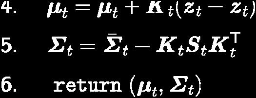
 t t t t t Updated mean 7: Σ = I K H Σ")

11 EKF_known_correspondence_localization (,, u, z, c, m) μt Σ 1 t 1 t t t Correction 2 2 ( m μ, ) + 1: ˆ x t x ( m μ y t, y) z = t ( m μ, m μ y t, y x t, x) μ atan2 t, θ Predicted measurement mean 2: r r r t t t h( μ, m) t μ μ μ tx, ty, t, θ H = = t x φ φ φ t t t t μ μ μ tx, ty, t, θ Jacobian of h wrt location 3: 2 σ 0 r Q = t 2 0 σ r 4: S = H Σ H + Q Predicted measurement covariance t t t t t T 1 5: K = Σ H S Kalman gain t t t t 6: μ = μ + K ( z zˆ ) t t t t t Updated mean 7: Σ = I K H Σ Updated covariance ( ) t t t t Basilio Bona June EKF prediction step different motion noise parameters Small rotation and translation noise High rotation noise High translation noise High rotation and translation noise Basilio Bona June

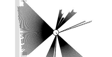
12 EKF measurement prediction step innovation z zˆ t t innovation Basilio Bona June EKF correction step measurement uncertainty uncertainty in robot location Prediction uncertainty Basilio Bona June


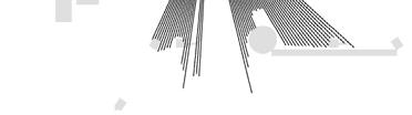
13 Estimation Sequence (1) Accurate detection sensor trajectories estimated from the motion control uncertainty ground truth trajectories before corrected trajectories after Basilio Bona June Estimation Sequence (2) Less accurate detection sensor Basilio Bona June
14 Estimation with unknown correspondences When landmark correspondence is not certain (as it is often the case) one should adopt a strategy to determine the identity of the landmarks during localization The most simple and popular technique is the maximum likelihood correspondence One determines the most likely value of the correspondence variable c t and uses it as the true one This strategy is fragile when different landmarks have equally likely values How to reduce the risk Choose landmarks that are far apart, so not to be confused Make sure that the robot pose uncertainty remains small Basilio Bona June ML data association The maximum likelihood estimator (MLE) determines the correspondence c t that maximizes the likelihood cˆ = arg max p( z c, z, u, m) t t 1: t 1: t 1 1: t c t This expression is conditioned on all prior correspondences that are treated as always correct c1: t 1 When the number of landmarks is high, the number of possible correspondence grows too much and the problem becomes intractable A solution is to maximize each term singularly and then proceed as in cˆ = arg max p( z c, z, u, m) i i t t 1: t 1: t 1 1: t i ct i i Nz hμ c m HΣ H T + Q t t t t t t t i ct arg max ( ; (,, ), ) Basilio Bona June

15 Multi hypothesis tracking filter (MHTF) Each color represents a different hypothesis Basilio Bona June Localization with MHTF Current belief is represented not one but multiple hypotheses Each hypothesis is tracked by a Kalman filter Additional problems: Data association: which observation corresponds to which hypothesis? Hypothesis management: when it is necessary to add or delete hypotheses? Large body of literature on target tracking, motion correspondence etc. Basilio Bona June
16 MHTF example The blue robot sees a door, but cannot resolve withcertaintyits its position since also the other hypotheses (in red) are likely Basilio Bona June MHT (1) Hypotheses are extracted from laser range finder (LRF) scans H = { x ˆ, Σ, PH ( )} i i i i Each hypothesis is computed by pose estimate, covariance matrix and probability of being the correct one: Hypothesis probability is computed using Bayes rule sensor report Pr ( H) PH ( ) t i i PH ( r) = i t Pr () Hypotheses with low probability bbl are dl deletedd New candidates are extracted from LRF scans t C = {, z R} j j j Basilio Bona June
17 MHT (2) Basilio Bona June MHT (3) Basilio Bona June

 is")
18 MHT: Implemented System (3) Example run # hypotheses P(H best ) Map and trajectory #hypotheses vs. time Basilio Bona June UKF localization The UKF localization algorithm uses the unscented transform to linearize i the motion and the measurement models Instead of computing Jacobians of these models it computes Gaussians using sigma points and transforms them through the model The landmark association (correspondence) is certain Basilio Bona June


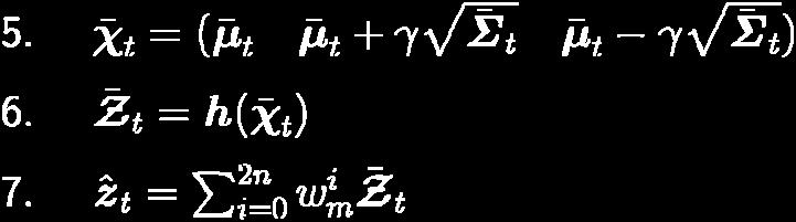
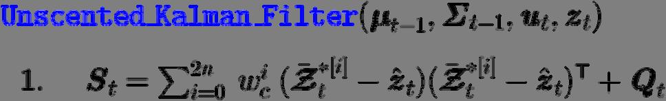


19 UKF Algorithm part a) Sigma points Basilio Bona June UKF Algorithm part b) Cross covariance Basilio Bona June
20 UKF_localization (,, u, z, m) μt Σ 1 t 1 t t 2 ( α v 1 2 ) 0 t + α ωt M = t 2 0 ( α v α ω Motion noise + 3 t 4 t ) 2 σ 0 r Q = Measurement noise t 2 0 σ r T T a T μ = μ 1 1 ( 00) ( 00 t t ) Σ 0 0 t 1 a Σ = 0 M 0 t 1 t Augmented covariance 0 0 Qt ( ) χ = μ μ + γ Σ μ γ Σ χ a a a a a a t 1 t 1 t 1 t 1 t 1 t 1 x t = g( χ) Prediction of sigma points PREDICTION Augmented state mean Sigma points 2L i x μ = t w χ m i, t Predicted mean i= 0 2L T i x x Σ = w t c ( χ μ i, t t) ( χ μ i, t t) Predicted covariance i= 0 Basilio Bona June x ( ) Ζ = h χ + χ UKF_localization ( (,,, u, u, z,, zm, m) ) z t t t μ μ t Σ 1t Σ 1 t 1t 1 t t t t CORRECTION 1) Measurement sigma points 2L i zˆ = t w Ζ m i, t Predicted measurement mean i= 0 ( Ζ ˆ)( Ζ ˆ) 2L T i = t c i, t t i, t t i= 0 S w z z ( )( zˆ,, ) 2L T xz, i x = t w c i t t i t t i= 0 Σ χ μ Ζ Pred. measurement covariance Cross covariance K = Σ S xz, 1 t t t Kalman gain μ = μ + K ( z zˆ ) t t t t t Σ = Σ KSK T t t t t t Updated mean Updated covariance Basilio Bona June
 Basilio Bona June 2011 41 UKF Prediction Step 3) High noise in rotation small in translation 1) Small noise in")
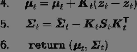
21 zˆ t 2 2 ( m μ, ) + ( m μ x t x y t, y) = Predicted measurement mean atan 2 ( m μ, m μ y t, y x t, x) μ t, θ r r r t t t h( μ, m) t μ μ μ tx, ty, t, θ H = = t x φ φ φ Jacobian of h w.r.t. location t t t t μ μ μ tx, ty, t, θ 2 σ 0 r Q = t 2 0 σ r S = H Σ H + Q T t t t t t K μ = μ + K ( z zˆ ) Σ = Σ H S T 1 t t t t t t t t t ( I K H ) Σt = t t t Pred. measurement covariance Kalman gain Updated mean Updated covariance CORRECTION 2) Basilio Bona June UKF Prediction Step 3) High noise in rotation small in translation 1) Small noise in translation and rotation Initial estimate 2) High noise in translation small in rotation 4) High noise in translation and in rotation Basilio Bona June


22 UKF Observation Prediction Step The left plots show the sigma points predicted from two motion updates along with the resulting uncertainty ellipses. The true robot and the observation are indicated by the white circle and the bold line, respectively The right plots show the resulting li measurement prediction sigma points. The white arrows indicate the innovations, the differences between observed and predicted measurements Basilio Bona June UKF Correction Step The panels on the left show the measurement prediction The panels on the right the resulting corrections, which update the mean estimate and reduce the position uncertainty ellipses Basilio Bona June
")

23 EKF Correction Step Basilio Bona June Estimation Sequence Robot trajectory according to the motion control (dashed lines) and the resulting true trajectory (solid lines) Landmark detections are indicated by thin lines EKF PF UKF Basilio Bona June

24 Prediction Quality EKF prediction UKF prediction Approximation error due to linearization The robot moves on a circle The reference covariances are extracted from an accurate, sample based prediction Basilio Bona June Mobile robot localization Grid and Monte Carlo methods These algorithms can process raw sensor measurement, i.e., there is no need to extract features from measurements These methods are non parametric, e.g., they are not limited to unimodal distributions as with the EKF localization method They can solve global localization problem and kidnapped robot problems (in some cases); the EKF algorithm is not able to solve such problems The first method is called grid localization The second method is called Monte Carlo localization Basilio Bona June

 Measurement model Correction/update step Motion model (prediction) Basilio Bona")
25 Grid localization Grid localization uses a histogram filter to represent posterior belief The grid dimension is a key factor for the performances of the method When the cell grid dimension is small, the algorithm can be extremely slow When the cell grid dimension is large, there can be an information loss that makes the algorithm not working in some cases Basilio Bona June Example Measurement model Correction/update step Motion model (prediction) Measurement model Correction/update step Motion model (prediction) Basilio Bona June
 exist Humans manage spatial knowledge primarily by topological information This information is used to construct a hierarchical topological map that describes the environment Basilio Bona June")
26 Topological grid map A topological map is a graph annotation of the environment Topological maps assign nodes to particular places and edges as paths if direct passage between pairs of places (end nodes) exist Humans manage spatial knowledge primarily by topological information This information is used to construct a hierarchical topological map that describes the environment Basilio Bona June Topological grid map Topological grid map representation: Coarse gridding Cells of varying size Resolution influenced by the structure of the environment (significant places and landmarks as doors, corridors windows, T junctions, dead ends, act as grid elements) Grid elements Basilio Bona June
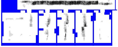
27 Metric grid map Metric grid representation: Finer gridding Cells of uniform size Resolution not influenced by the structure of the environment Usually cell sizes of 15 cm x 15 cm up to 1 m x 1m Motion model affected by robot velocity and cell size θ Basilio Bona June Cell size influence Cell size influence the performance of the grid localization algorithm Average localization error as a function of grid cell size, for ultrasound sensors and laser range finders Average CPU time needed for global localization as a function of grid resolution, shown for both ultrasound sensors and laser range finders Basilio Bona June


28 Example with metric grids 1 Basilio Bona June Example with metric grids 2 Basilio Bona June


29 Example with metric grids 3 Basilio Bona June Example with sonar data 1 Basilio Bona June

30 Example with sonar data 2 Basilio Bona June Example with sonar data 3 Basilio Bona June


31 Example with sonar data 4 Basilio Bona June Example with sonar data 5 Basilio Bona June
32 Monte Carlo localization Monte Carlo localization (MCL) is a relatively new, yet very popular algorithm It is a versatile method, where the belief is represented by a set of particles (i.e., a particle filter) ) It can be used both for local and for global localization problems In the context of localization, the particles are propagated according to the motion model They are then weighted according to the likelihood of the observations In a re sampling step, new particles il are drawn with iha probability proportional to the likelihood of the observation The method first appeared in 70 s, and was re discovered by Kitagawa and Isard & Blake in computer vision Basilio Bona June Particle filter localization (MCL) Particle filters based localization (Monte Carlo Localization MCL) uses a set of weighted random samples to approximate the robot pose belief Particle set size n ( ) [] i ( ˆ [] i t ω δ t t t ) bel p p p i= 1 n with i= 1 ω [] i t = 1 Pose of the particle Weight of the particle Basilio Bona June
33 Particle filter localization (MCL) Particle based Representation of position belief Particle based approximation Gaussian approximation (ellipse: 95% acceptance region) Basilio Bona June Particle filter localization (MCL) Using particle filters approximation, the Bayes Filter can be reformulated as follows (starting from the robot initial belief at time zero) 1. PREDICTION: Generate a new set of particles given the motion model and the applied controls 2. UPDATE: Assign to each particle an importance weight according to the sensor measurements 3. RESAMPLING: Randomly resample particles in function of their importance weight Basilio Bona June
 t t t t The variable is randomly extracted according to the noise distribution We obtain a set of predicted")
 t t Particles whose predictions match the measurements are given a high weight In red the particles with high weights Basilio Bona June")
34 Prediction Prediction Generate a new set of particles given the motion model and the applied controls For each particle: Given the particle pose at time step t-1 and the commands, the particle pose at time t is predicted using the motion model [] i [] i pˆ = f pˆ, u, ω ( 1 ) t t t t The variable is randomly extracted according to the noise distribution We obtain a set of predicted particles Basilio Bona June Update Update Assign to each particle an importance weight according to the sensor measurements For each particle: Compare particle s prediction of measurements with actual [ i ] measurements z vs h( pˆ ) t t Particles whose predictions match the measurements are given a high weight In red the particles with high weights Basilio Bona June

 Measurement model Correction/update step Motion model (prediction) Basilio Bona")
35 Resampling Resampling Randomly resample particles in function of their importance weight For each particle: For n times draw (with replacement) a particle from Γ t with probability given by the importance weights and put it in the set Γ t Particles whose predictions match the measurements are given a high weight The new set Γ t provides the particle based approximation of the robot pose at time t Basilio Bona June Example Measurement model Correction/update step Motion model (prediction) Measurement model Correction/update step Motion model (prediction) Basilio Bona June
 [ m] t t [ m] t 1 [ m] [ m] = measurement_model t t t [ m] [")
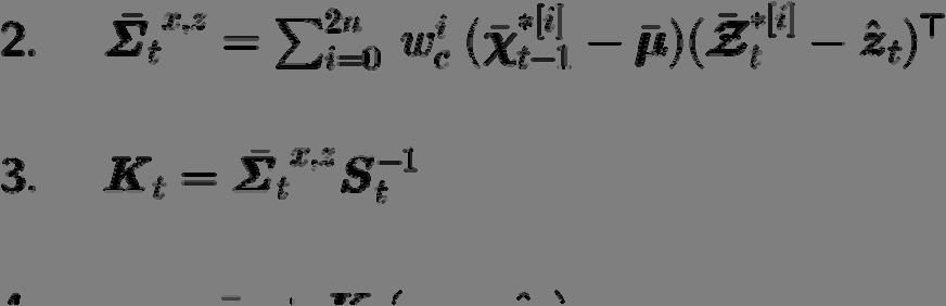
![m] = χ + x w t t t t 4: w ( z, x, m) 5: χ, 6: endfor 7: for m = 1to M do 8: 9: 10: endfor draw i with](/docs-images/79/78948702/images/36-2.jpg "probability add x [] i t to χ t w [] i t 11 : return χt see previous slides Basilio Bona June 2011 72")
36 Example Basilio Bona June MC_localization ( χ,,, ) t u z m 1 t t 1: χ t = χ = 2: for m = 1to M do t 3: x = sample_motion_model ( u, x ) [ m] t t [ m] t 1 [ m] [ m] = measurement_model t t t [ m] [ m] = χ + x w t t t t 4: w ( z, x, m) 5: χ, 6: endfor 7: for m = 1to M do 8: 9: 10: endfor draw i with probability add x [] i t to χ t w [] i t 11 : return χt see previous slides Basilio Bona June
37 Monte Carlo Localization within a sensor infrastructure Fixed sensors deployed in known positions in the environment STEP 1: Basilio Bona June STEP 1: Basilio Bona June
38 STEP 1: Acquire meas. Basilio Bona June STEP 1: Acquire meas. Weights Update Basilio Bona June
39 STEP 1: Acquire meas. Weights Update Resampling Basilio Bona June STEP 1: Acquire meas. Weights Update Resampling STEP 1: Basilio Bona June
40 STEP 1: Acquire meas. Weights Update Resampling STEP 1: Basilio Bona June STEP 1: Acquire meas. Weights Update Resampling STEP 2: Acquire meas. Basilio Bona June
41 STEP 1: Acquire meas. Weights Update Resampling STEP 2: Acquire meas. Weights Update Basilio Bona June STEP 1: Acquire meas. Weights Update Resampling STEP 2: Acquire meas. Weights Update Resampling Basilio Bona June
42 STEP 1: Acquire meas. Weights Update Resampling STEP 2: Acquire meas. Weights Update Resampling STEP 3: Basilio Bona June STEP 1: Acquire meas. Weights Update Resampling STEP 2: Acquire meas. Weights Update Resampling STEP 3: Basilio Bona June
43 STEP 1: Acquire meas. Weights Update Resampling STEP 2: Acquire meas. Weights Update Resampling STEP 3: Acquire meas. Basilio Bona June STEP 1: Acquire meas. Weights Update Resampling STEP 2: Acquire meas. Weights Update Resampling STEP 3: Acquire meas. Weights Update Basilio Bona June


44 STEP 1: Acquire meas. Weights Update Resampling STEP 2: Acquire meas. Weights Update Resampling STEP 3: Acquire meas. Weights Update Resampling Basilio Bona June Example for landmark based localization Basilio Bona June

45 Properties of MCL MCL can approximate any distribution, as it can represent complex multi modal distributions and blend them with Gaussian style distributions Increasing the total number of particles increases the accuracy of the approximation The number of particles M is a trade off parameter between accuracy and necessary computational resources Particles number shall remain large enough to avoid filter divergence The particles number may remain fixed or change adaptively Basilio Bona June Adapting the particle size In the example below, the number of particles is very high ( ) to allow an accurate representation of the belief during early stages of the algorithm, but is unnecessarily high in later stages, when the belief concentrates in smaller regions an adaptive strategy is required Basilio Bona June
46 KLD sampling Kullback Leibler divergence (KLD) sampling is a variant of MCL that adapts the number of particles over time KLD (also known as information divergence, information gain, relative entropy)is a measure of the difference between two probability distributions For probability distributions P and Q of adiscrete random variable their KLD is defined as For distributions P and Q of a continuous random variable, the KLD is defined as an integral Basilio Bona June KLD sampling The idea is to set adaptively the number of particles based on a statistical bound on the sample based approximation quality At each iteration of the PF, KLD sampling determines the number of samples such that, with probability 1 d, the error between the true posterior and the sample based approximation is less than ε To derive this bound, we assume that the true posterior is given by a discrete, piecewise constant distribution such as a discrete density tree or a multi dimensional histogram Basilio Bona June
")
 distribution 1 δ Basilio Bona")
47 KLD sampling Basilio Bona June Approximation formula n k z 2ε 9( k 1) 9( k 1) 1 δ 3 where z is the upper 1 δ quantile of the normal N(0,1) distribution 1 δ Basilio Bona June
48 Dynamic environment Markov assumptions are good for a static environment Oftenthe the environment where robots operate is full of people moving randomly People dynamics is not modeled by the state x t Probabilistic approaches are robust since they incorporate sensor noise, but... sensor noise must be independent at each time step... while people dynamics is highly dependent in time Basilio Bona June Dynamic environment: which solution State Augmentation include the hidden state into the state estimated by the filter it is more general, but suffer from high computational complexity: the pose of each subject moving around the robot must be estimated, and the number of states varies in time Outlier rejection pre process sensor measurements to eliminate measurements affected by hidden state it may work well when the people presence affects the sensors (laser range finder, and, to lesser extent, vision sensors) reading Basilio Bona June
49 Outlier rejection The Expectation maximization (EM) learning algorithm is used for outlier detection and rejection It comes from the beam model of range finders, where z unexp and p unexp parameters relates to unexpectedobjects we have to introduce and compute a correspondence variable that can take one of four values {hit, short, max, rand} the desired probability is computed as this integral does not have a closed form solution k p ( z x, m) z bel( x )dx k k unexp t t unexp t t pc ( = unexp z, z, u, m) = t t 1: t 1 1: t k p ( z x, m) z bel( x )dx c t t c t t c approximation with a representative sample of the posterior k c t the measurement is rejected if the probability exceeds a given threshold Basilio Bona June Comparison of different ML implementations EKF MHT Topological grid Metric grid MCL Measurements landmarks landmarks landmarks Measurement noise raw measurements raw measurements Gaussian Gaussian any any any Posterior Gaussian mixture of Gaussians histogram histogram particles Efficiency (mem) Efficiency (time) Ease of implementation i Resolution Robustness Global localization no no yes yes yes Basilio Bona June
Probabilistic Fundamentals in Robotics. DAUIN Politecnico di Torino July 2010
 Probabilistic Fundamentals in Robotics Probabilistic Models of Mobile Robots Robot localization Basilio Bona DAUIN Politecnico di Torino July 2010 Course Outline Basic mathematical framework Probabilistic
Probabilistic Fundamentals in Robotics. DAUIN Politecnico di Torino July 2010
 Probabilistic Fundamentals in Robotics Gaussian Filters Basilio Bona DAUIN Politecnico di Torino July 2010 Course Outline Basic mathematical framework Probabilistic models of mobile robots Mobile robot
ROBOTICS 01PEEQW. Basilio Bona DAUIN Politecnico di Torino
 ROBOTICS 01PEEQW Basilio Bona DAUIN Politecnico di Torino Probabilistic Fundamentals in Robotics Gaussian Filters Course Outline Basic mathematical framework Probabilistic models of mobile robots Mobile
Introduction to Mobile Robotics Bayes Filter Particle Filter and Monte Carlo Localization
 Introduction to Mobile Robotics Bayes Filter Particle Filter and Monte Carlo Localization Wolfram Burgard, Cyrill Stachniss, Maren Bennewitz, Kai Arras 1 Motivation Recall: Discrete filter Discretize the
2D Image Processing (Extended) Kalman and particle filter
 Kalman and particle filter") 2D Image Processing (Extended) Kalman and particle filter Prof. Didier Stricker Dr. Gabriele Bleser Kaiserlautern University http://ags.cs.uni-kl.de/ DFKI Deutsches Forschungszentrum für Künstliche Intelligenz
2D Image Processing (Extended) Kalman and particle filter Prof. Didier Stricker Dr. Gabriele Bleser Kaiserlautern University http://ags.cs.uni-kl.de/ DFKI Deutsches Forschungszentrum für Künstliche Intelligenz
Probabilistic Fundamentals in Robotics. DAUIN Politecnico di Torino July 2010
 Probabilistic Fundamentals in Robotics Probabilistic Models of Mobile Robots Robotic mapping Basilio Bona DAUIN Politecnico di Torino July 2010 Course Outline Basic mathematical framework Probabilistic
Mobile Robot Localization
 Mobile Robot Localization 1 The Problem of Robot Localization Given a map of the environment, how can a robot determine its pose (planar coordinates + orientation)? Two sources of uncertainty: - observations
Robotics. Mobile Robotics. Marc Toussaint U Stuttgart
 Robotics Mobile Robotics State estimation, Bayes filter, odometry, particle filter, Kalman filter, SLAM, joint Bayes filter, EKF SLAM, particle SLAM, graph-based SLAM Marc Toussaint U Stuttgart DARPA Grand
Recursive Bayes Filtering
 Recursive Bayes Filtering CS485 Autonomous Robotics Amarda Shehu Fall 2013 Notes modified from Wolfram Burgard, University of Freiburg Physical Agents are Inherently Uncertain Uncertainty arises from four
The Particle Filter. PD Dr. Rudolph Triebel Computer Vision Group. Machine Learning for Computer Vision
 The Particle Filter Non-parametric implementation of Bayes filter Represents the belief (posterior) random state samples. by a set of This representation is approximate. Can represent distributions that
Introduction to Mobile Robotics Probabilistic Sensor Models
 Introduction to Mobile Robotics Probabilistic Sensor Models Wolfram Burgard 1 Sensors for Mobile Robots Contact sensors: Bumpers Proprioceptive sensors Accelerometers (spring-mounted masses) Gyroscopes
Particle Filters. Pieter Abbeel UC Berkeley EECS. Many slides adapted from Thrun, Burgard and Fox, Probabilistic Robotics
 Particle Filters Pieter Abbeel UC Berkeley EECS Many slides adapted from Thrun, Burgard and Fox, Probabilistic Robotics Motivation For continuous spaces: often no analytical formulas for Bayes filter updates
Modeling and state estimation Examples State estimation Probabilities Bayes filter Particle filter. Modeling. CSC752 Autonomous Robotic Systems
 Modeling CSC752 Autonomous Robotic Systems Ubbo Visser Department of Computer Science University of Miami February 21, 2017 Outline 1 Modeling and state estimation 2 Examples 3 State estimation 4 Probabilities
Mobile Robot Localization
 Mobile Robot Localization 1 The Problem of Robot Localization Given a map of the environment, how can a robot determine its pose (planar coordinates + orientation)? Two sources of uncertainty: - observations
Simultaneous Localization and Mapping
 Simultaneous Localization and Mapping Miroslav Kulich Intelligent and Mobile Robotics Group Czech Institute of Informatics, Robotics and Cybernetics Czech Technical University in Prague Winter semester
SLAM Techniques and Algorithms. Jack Collier. Canada. Recherche et développement pour la défense Canada. Defence Research and Development Canada
 SLAM Techniques and Algorithms Jack Collier Defence Research and Development Canada Recherche et développement pour la défense Canada Canada Goals What will we learn Gain an appreciation for what SLAM
L11. EKF SLAM: PART I. NA568 Mobile Robotics: Methods & Algorithms
 L11. EKF SLAM: PART I NA568 Mobile Robotics: Methods & Algorithms Today s Topic EKF Feature-Based SLAM State Representation Process / Observation Models Landmark Initialization Robot-Landmark Correlation
Computer Vision Group Prof. Daniel Cremers. 11. Sampling Methods
 Prof. Daniel Cremers 11. Sampling Methods Sampling Methods Sampling Methods are widely used in Computer Science as an approximation of a deterministic algorithm to represent uncertainty without a parametric
Robot Localisation. Henrik I. Christensen. January 12, 2007
 Robot Henrik I. Robotics and Intelligent Machines @ GT College of Computing Georgia Institute of Technology Atlanta, GA hic@cc.gatech.edu January 12, 2007 The Robot Structure Outline 1 2 3 4 Sum of 5 6
Particle Filters; Simultaneous Localization and Mapping (Intelligent Autonomous Robotics) Subramanian Ramamoorthy School of Informatics
 Subramanian Ramamoorthy School of Informatics") Particle Filters; Simultaneous Localization and Mapping (Intelligent Autonomous Robotics) Subramanian Ramamoorthy School of Informatics Recap: State Estimation using Kalman Filter Project state and error
Particle Filters; Simultaneous Localization and Mapping (Intelligent Autonomous Robotics) Subramanian Ramamoorthy School of Informatics Recap: State Estimation using Kalman Filter Project state and error
CSE 473: Artificial Intelligence
 CSE 473: Artificial Intelligence Hidden Markov Models Dieter Fox --- University of Washington [Most slides were created by Dan Klein and Pieter Abbeel for CS188 Intro to AI at UC Berkeley. All CS188 materials
Computer Vision Group Prof. Daniel Cremers. 14. Sampling Methods
 Prof. Daniel Cremers 14. Sampling Methods Sampling Methods Sampling Methods are widely used in Computer Science as an approximation of a deterministic algorithm to represent uncertainty without a parametric
Bayes Filter Reminder. Kalman Filter Localization. Properties of Gaussians. Gaussians. Prediction. Correction. σ 2. Univariate. 1 2πσ e.
 Kalman Filter Localization Bayes Filter Reminder Prediction Correction Gaussians p(x) ~ N(µ,σ 2 ) : Properties of Gaussians Univariate p(x) = 1 1 2πσ e 2 (x µ) 2 σ 2 µ Univariate -σ σ Multivariate µ Multivariate
Bayesian Methods / G.D. Hager S. Leonard
 Bayesian Methods Recall Robot Localization Given Sensor readings z 1, z 2,, z t = z 1:t Known control inputs u 0, u 1, u t = u 0:t Known model t+1 t, u t ) with initial 1 u 0 ) Known map z t t ) Compute
Introduction to Mobile Robotics SLAM: Simultaneous Localization and Mapping
 Introduction to Mobile Robotics SLAM: Simultaneous Localization and Mapping Wolfram Burgard, Cyrill Stachniss, Kai Arras, Maren Bennewitz What is SLAM? Estimate the pose of a robot and the map of the environment
ECE276A: Sensing & Estimation in Robotics Lecture 10: Gaussian Mixture and Particle Filtering
 ECE276A: Sensing & Estimation in Robotics Lecture 10: Gaussian Mixture and Particle Filtering Lecturer: Nikolay Atanasov: natanasov@ucsd.edu Teaching Assistants: Siwei Guo: s9guo@eng.ucsd.edu Anwesan Pal:
Robots Autónomos. Depto. CCIA. 2. Bayesian Estimation and sensor models. Domingo Gallardo
 Robots Autónomos 2. Bayesian Estimation and sensor models Domingo Gallardo Depto. CCIA http://www.rvg.ua.es/master/robots References Recursive State Estimation: Thrun, chapter 2 Sensor models and robot
Markov localization uses an explicit, discrete representation for the probability of all position in the state space.
 Markov Kalman Filter Localization Markov localization localization starting from any unknown position recovers from ambiguous situation. However, to update the probability of all positions within the whole
CIS 390 Fall 2016 Robotics: Planning and Perception Final Review Questions
 CIS 390 Fall 2016 Robotics: Planning and Perception Final Review Questions December 14, 2016 Questions Throughout the following questions we will assume that x t is the state vector at time t, z t is the
Sensor Tasking and Control
 Sensor Tasking and Control Sensing Networking Leonidas Guibas Stanford University Computation CS428 Sensor systems are about sensing, after all... System State Continuous and Discrete Variables The quantities
PATTERN RECOGNITION AND MACHINE LEARNING CHAPTER 13: SEQUENTIAL DATA
 PATTERN RECOGNITION AND MACHINE LEARNING CHAPTER 13: SEQUENTIAL DATA Contents in latter part Linear Dynamical Systems What is different from HMM? Kalman filter Its strength and limitation Particle Filter
Robot Localization and Kalman Filters
 Robot Localization and Kalman Filters Rudy Negenborn rudy@negenborn.net August 26, 2003 Outline Robot Localization Probabilistic Localization Kalman Filters Kalman Localization Kalman Localization with
Autonomous Mobile Robot Design
 Autonomous Mobile Robot Design Topic: Extended Kalman Filter Dr. Kostas Alexis (CSE) These slides relied on the lectures from C. Stachniss, J. Sturm and the book Probabilistic Robotics from Thurn et al.
Robotics 2 Target Tracking. Kai Arras, Cyrill Stachniss, Maren Bennewitz, Wolfram Burgard
 Robotics 2 Target Tracking Kai Arras, Cyrill Stachniss, Maren Bennewitz, Wolfram Burgard Slides by Kai Arras, Gian Diego Tipaldi, v.1.1, Jan 2012 Chapter Contents Target Tracking Overview Applications
2D Image Processing. Bayes filter implementation: Kalman filter
 2D Image Processing Bayes filter implementation: Kalman filter Prof. Didier Stricker Kaiserlautern University http://ags.cs.uni-kl.de/ DFKI Deutsches Forschungszentrum für Künstliche Intelligenz http://av.dfki.de
EKF and SLAM. McGill COMP 765 Sept 18 th, 2017
 EKF and SLAM McGill COMP 765 Sept 18 th, 2017 Outline News and information Instructions for paper presentations Continue on Kalman filter: EKF and extension to mapping Example of a real mapping system:
Introduction to Machine Learning
 Introduction to Machine Learning Brown University CSCI 1950-F, Spring 2012 Prof. Erik Sudderth Lecture 25: Markov Chain Monte Carlo (MCMC) Course Review and Advanced Topics Many figures courtesy Kevin
Autonomous Mobile Robot Design
 Autonomous Mobile Robot Design Topic: Particle Filter for Localization Dr. Kostas Alexis (CSE) These slides relied on the lectures from C. Stachniss, and the book Probabilistic Robotics from Thurn et al.
2D Image Processing. Bayes filter implementation: Kalman filter
 2D Image Processing Bayes filter implementation: Kalman filter Prof. Didier Stricker Dr. Gabriele Bleser Kaiserlautern University http://ags.cs.uni-kl.de/ DFKI Deutsches Forschungszentrum für Künstliche
Linear Dynamical Systems
 Linear Dynamical Systems Sargur N. srihari@cedar.buffalo.edu Machine Learning Course: http://www.cedar.buffalo.edu/~srihari/cse574/index.html Two Models Described by Same Graph Latent variables Observations
AUTOMOTIVE ENVIRONMENT SENSORS
 AUTOMOTIVE ENVIRONMENT SENSORS Lecture 5. Localization BME KÖZLEKEDÉSMÉRNÖKI ÉS JÁRMŰMÉRNÖKI KAR 32708-2/2017/INTFIN SZÁMÚ EMMI ÁLTAL TÁMOGATOTT TANANYAG Related concepts Concepts related to vehicles moving
Lecture 2: From Linear Regression to Kalman Filter and Beyond
 Lecture 2: From Linear Regression to Kalman Filter and Beyond January 18, 2017 Contents 1 Batch and Recursive Estimation 2 Towards Bayesian Filtering 3 Kalman Filter and Bayesian Filtering and Smoothing
Partially Observable Markov Decision Processes (POMDPs)
") Partially Observable Markov Decision Processes (POMDPs) Sachin Patil Guest Lecture: CS287 Advanced Robotics Slides adapted from Pieter Abbeel, Alex Lee Outline Introduction to POMDPs Locally Optimal Solutions
Partially Observable Markov Decision Processes (POMDPs) Sachin Patil Guest Lecture: CS287 Advanced Robotics Slides adapted from Pieter Abbeel, Alex Lee Outline Introduction to POMDPs Locally Optimal Solutions
From Bayes to Extended Kalman Filter
 From Bayes to Extended Kalman Filter Michal Reinštein Czech Technical University in Prague Faculty of Electrical Engineering, Department of Cybernetics Center for Machine Perception http://cmp.felk.cvut.cz/
Lecture 2: From Linear Regression to Kalman Filter and Beyond
 Lecture 2: From Linear Regression to Kalman Filter and Beyond Department of Biomedical Engineering and Computational Science Aalto University January 26, 2012 Contents 1 Batch and Recursive Estimation
Mathematical Formulation of Our Example
 Mathematical Formulation of Our Example We define two binary random variables: open and, where is light on or light off. Our question is: What is? Computer Vision 1 Combining Evidence Suppose our robot
Efficient Monitoring for Planetary Rovers
 International Symposium on Artificial Intelligence and Robotics in Space (isairas), May, 2003 Efficient Monitoring for Planetary Rovers Vandi Verma vandi@ri.cmu.edu Geoff Gordon ggordon@cs.cmu.edu Carnegie
A Comparison of the EKF, SPKF, and the Bayes Filter for Landmark-Based Localization
 A Comparison of the EKF, SPKF, and the Bayes Filter for Landmark-Based Localization and Timothy D. Barfoot CRV 2 Outline Background Objective Experimental Setup Results Discussion Conclusion 2 Outline
Chapter 9: Bayesian Methods. CS 336/436 Gregory D. Hager
 Chapter 9: Bayesian Methods CS 336/436 Gregory D. Hager A Simple Eample Why Not Just Use a Kalman Filter? Recall Robot Localization Given Sensor readings y 1, y 2, y = y 1: Known control inputs u 0, u
Probabilistic Graphical Models
 Probabilistic Graphical Models Brown University CSCI 2950-P, Spring 2013 Prof. Erik Sudderth Lecture 13: Learning in Gaussian Graphical Models, Non-Gaussian Inference, Monte Carlo Methods Some figures
Target Tracking and Classification using Collaborative Sensor Networks
 Target Tracking and Classification using Collaborative Sensor Networks Xiaodong Wang Department of Electrical Engineering Columbia University p.1/3 Talk Outline Background on distributed wireless sensor
Probabilistic Graphical Models
 Probabilistic Graphical Models Brown University CSCI 295-P, Spring 213 Prof. Erik Sudderth Lecture 11: Inference & Learning Overview, Gaussian Graphical Models Some figures courtesy Michael Jordan s draft
Parametric Unsupervised Learning Expectation Maximization (EM) Lecture 20.a
 Lecture 20.a") Parametric Unsupervised Learning Expectation Maximization (EM) Lecture 20.a Some slides are due to Christopher Bishop Limitations of K-means Hard assignments of data points to clusters small shift of a
Parametric Unsupervised Learning Expectation Maximization (EM) Lecture 20.a Some slides are due to Christopher Bishop Limitations of K-means Hard assignments of data points to clusters small shift of a
Introduction to Mobile Robotics Information Gain-Based Exploration. Wolfram Burgard, Cyrill Stachniss, Maren Bennewitz, Giorgio Grisetti, Kai Arras
 Introduction to Mobile Robotics Information Gain-Based Exploration Wolfram Burgard, Cyrill Stachniss, Maren Bennewitz, Giorgio Grisetti, Kai Arras 1 Tasks of Mobile Robots mapping SLAM localization integrated
TSRT14: Sensor Fusion Lecture 8
 TSRT14: Sensor Fusion Lecture 8 Particle filter theory Marginalized particle filter Gustaf Hendeby gustaf.hendeby@liu.se TSRT14 Lecture 8 Gustaf Hendeby Spring 2018 1 / 25 Le 8: particle filter theory,
Robotics 2 Data Association. Giorgio Grisetti, Cyrill Stachniss, Kai Arras, Wolfram Burgard
 Robotics 2 Data Association Giorgio Grisetti, Cyrill Stachniss, Kai Arras, Wolfram Burgard Data Association Data association is the process of associating uncertain measurements to known tracks. Problem
Variable Resolution Particle Filter
 In Proceedings of the International Joint Conference on Artificial intelligence (IJCAI) August 2003. 1 Variable Resolution Particle Filter Vandi Verma, Sebastian Thrun and Reid Simmons Carnegie Mellon
Approximate Inference
 Approximate Inference Simulation has a name: sampling Sampling is a hot topic in machine learning, and it s really simple Basic idea: Draw N samples from a sampling distribution S Compute an approximate
Content.
 Content Fundamentals of Bayesian Techniques (E. Sucar) Bayesian Filters (O. Aycard) Definition & interests Implementations Hidden Markov models Discrete Bayesian Filters or Markov localization Kalman filters
Rao-Blackwellized Particle Filter for Multiple Target Tracking
 Rao-Blackwellized Particle Filter for Multiple Target Tracking Simo Särkkä, Aki Vehtari, Jouko Lampinen Helsinki University of Technology, Finland Abstract In this article we propose a new Rao-Blackwellized
Self Adaptive Particle Filter
 Self Adaptive Particle Filter Alvaro Soto Pontificia Universidad Catolica de Chile Department of Computer Science Vicuna Mackenna 4860 (143), Santiago 22, Chile asoto@ing.puc.cl Abstract The particle filter
CSEP 573: Artificial Intelligence
 CSEP 573: Artificial Intelligence Hidden Markov Models Luke Zettlemoyer Many slides over the course adapted from either Dan Klein, Stuart Russell, Andrew Moore, Ali Farhadi, or Dan Weld 1 Outline Probabilistic
Kalman filtering and friends: Inference in time series models. Herke van Hoof slides mostly by Michael Rubinstein
 Kalman filtering and friends: Inference in time series models Herke van Hoof slides mostly by Michael Rubinstein Problem overview Goal Estimate most probable state at time k using measurement up to time
Vlad Estivill-Castro. Robots for People --- A project for intelligent integrated systems
 1 Vlad Estivill-Castro Robots for People --- A project for intelligent integrated systems V. Estivill-Castro 2 Probabilistic Map-based Localization (Kalman Filter) Chapter 5 (textbook) Based on textbook
Introduction to Mobile Robotics Probabilistic Robotics
 Introduction to Mobile Robotics Probabilistic Robotics Wolfram Burgard 1 Probabilistic Robotics Key idea: Explicit representation of uncertainty (using the calculus of probability theory) Perception Action
Introduction to Mobile Robotics Probabilistic Motion Models
 Introduction to Mobile Robotics Probabilistic Motion Models Wolfram Burgard 1 Robot Motion Robot motion is inherently uncertain. How can we model this uncertainty? 2 Dynamic Bayesian Network for Controls,
E190Q Lecture 10 Autonomous Robot Navigation
 E190Q Lecture 10 Autonomous Robot Navigation Instructor: Chris Clark Semester: Spring 2015 1 Figures courtesy of Siegwart & Nourbakhsh Kilobots 2 https://www.youtube.com/watch?v=2ialuwgafd0 Control Structures
CS491/691: Introduction to Aerial Robotics
 CS491/691: Introduction to Aerial Robotics Topic: State Estimation Dr. Kostas Alexis (CSE) World state (or system state) Belief state: Our belief/estimate of the world state World state: Real state of
Probabilistic Graphical Models
 Probabilistic Graphical Models Lecture 12 Dynamical Models CS/CNS/EE 155 Andreas Krause Homework 3 out tonight Start early!! Announcements Project milestones due today Please email to TAs 2 Parameter learning
Why do we care? Measurements. Handling uncertainty over time: predicting, estimating, recognizing, learning. Dealing with time
 Handling uncertainty over time: predicting, estimating, recognizing, learning Chris Atkeson 2004 Why do we care? Speech recognition makes use of dependence of words and phonemes across time. Knowing where
SLAM for Ship Hull Inspection using Exactly Sparse Extended Information Filters
 SLAM for Ship Hull Inspection using Exactly Sparse Extended Information Filters Matthew Walter 1,2, Franz Hover 1, & John Leonard 1,2 Massachusetts Institute of Technology 1 Department of Mechanical Engineering
Using the Kalman Filter for SLAM AIMS 2015
 Using the Kalman Filter for SLAM AIMS 2015 Contents Trivial Kinematics Rapid sweep over localisation and mapping (components of SLAM) Basic EKF Feature Based SLAM Feature types and representations Implementation
L06. LINEAR KALMAN FILTERS. NA568 Mobile Robotics: Methods & Algorithms
 L06. LINEAR KALMAN FILTERS NA568 Mobile Robotics: Methods & Algorithms 2 PS2 is out! Landmark-based Localization: EKF, UKF, PF Today s Lecture Minimum Mean Square Error (MMSE) Linear Kalman Filter Gaussian
Mobile Robots Localization
 Mobile Robots Localization Institute for Software Technology 1 Today s Agenda Motivation for Localization Odometry Odometry Calibration Error Model 2 Robotics is Easy control behavior perception modelling
Bayesian Networks: Construction, Inference, Learning and Causal Interpretation. Volker Tresp Summer 2014
 Bayesian Networks: Construction, Inference, Learning and Causal Interpretation Volker Tresp Summer 2014 1 Introduction So far we were mostly concerned with supervised learning: we predicted one or several
Probabilistic Robotics
 Probabilisic Roboics Bayes Filer Implemenaions Gaussian filers Bayes Filer Reminder Predicion bel p u bel d Correcion bel η p z bel Gaussians : ~ π e p N p - Univariae / / : ~ μ μ μ e p Ν p d π Mulivariae
13: Variational inference II
 10-708: Probabilistic Graphical Models, Spring 2015 13: Variational inference II Lecturer: Eric P. Xing Scribes: Ronghuo Zheng, Zhiting Hu, Yuntian Deng 1 Introduction We started to talk about variational
Vlad Estivill-Castro (2016) Robots for People --- A project for intelligent integrated systems
 Robots for People --- A project for intelligent integrated systems") 1 Vlad Estivill-Castro (2016) Robots for People --- A project for intelligent integrated systems V. Estivill-Castro 2 Uncertainty representation Localization Chapter 5 (textbook) What is the course about?
1 Vlad Estivill-Castro (2016) Robots for People --- A project for intelligent integrated systems V. Estivill-Castro 2 Uncertainty representation Localization Chapter 5 (textbook) What is the course about?
Introduction to Mobile Robotics
 Inroducion o Mobile Roboics Bayes Filer Kalman Filer Wolfram Burgard Cyrill Sachniss Giorgio Grisei Maren Bennewiz Chrisian Plagemann Bayes Filer Reminder Predicion bel p u bel d Correcion bel η p z bel
L09. PARTICLE FILTERING. NA568 Mobile Robotics: Methods & Algorithms
 L09. PARTICLE FILTERING NA568 Mobile Robotics: Methods & Algorithms Particle Filters Different approach to state estimation Instead of parametric description of state (and uncertainty), use a set of state
PROBABILISTIC REASONING OVER TIME
 PROBABILISTIC REASONING OVER TIME In which we try to interpret the present, understand the past, and perhaps predict the future, even when very little is crystal clear. Outline Time and uncertainty Inference:
Bayesian Networks: Construction, Inference, Learning and Causal Interpretation. Volker Tresp Summer 2016
 Bayesian Networks: Construction, Inference, Learning and Causal Interpretation Volker Tresp Summer 2016 1 Introduction So far we were mostly concerned with supervised learning: we predicted one or several
Machine Learning Techniques for Computer Vision
 Machine Learning Techniques for Computer Vision Part 2: Unsupervised Learning Microsoft Research Cambridge x 3 1 0.5 0.2 0 0.5 0.3 0 0.5 1 ECCV 2004, Prague x 2 x 1 Overview of Part 2 Mixture models EM
Bayesian Methods for Machine Learning
 Bayesian Methods for Machine Learning CS 584: Big Data Analytics Material adapted from Radford Neal s tutorial (http://ftp.cs.utoronto.ca/pub/radford/bayes-tut.pdf), Zoubin Ghahramni (http://hunch.net/~coms-4771/zoubin_ghahramani_bayesian_learning.pdf),
Kalman Filter. Predict: Update: x k k 1 = F k x k 1 k 1 + B k u k P k k 1 = F k P k 1 k 1 F T k + Q
 Kalman Filter Kalman Filter Predict: x k k 1 = F k x k 1 k 1 + B k u k P k k 1 = F k P k 1 k 1 F T k + Q Update: K = P k k 1 Hk T (H k P k k 1 Hk T + R) 1 x k k = x k k 1 + K(z k H k x k k 1 ) P k k =(I
Stochastic Spectral Approaches to Bayesian Inference
 Stochastic Spectral Approaches to Bayesian Inference Prof. Nathan L. Gibson Department of Mathematics Applied Mathematics and Computation Seminar March 4, 2011 Prof. Gibson (OSU) Spectral Approaches to
Nonlinear and/or Non-normal Filtering. Jesús Fernández-Villaverde University of Pennsylvania
 Nonlinear and/or Non-normal Filtering Jesús Fernández-Villaverde University of Pennsylvania 1 Motivation Nonlinear and/or non-gaussian filtering, smoothing, and forecasting (NLGF) problems are pervasive
Sensor Fusion: Particle Filter
 Sensor Fusion: Particle Filter By: Gordana Stojceska stojcesk@in.tum.de Outline Motivation Applications Fundamentals Tracking People Advantages and disadvantages Summary June 05 JASS '05, St.Petersburg,
Simultaneous Localization and Mapping Techniques
 Simultaneous Localization and Mapping Techniques Andrew Hogue Oral Exam: June 20, 2005 Contents 1 Introduction 1 1.1 Why is SLAM necessary?.................................. 2 1.2 A Brief History of SLAM...................................
Probability Map Building of Uncertain Dynamic Environments with Indistinguishable Obstacles
 Probability Map Building of Uncertain Dynamic Environments with Indistinguishable Obstacles Myungsoo Jun and Raffaello D Andrea Sibley School of Mechanical and Aerospace Engineering Cornell University
1 Kalman Filter Introduction
 1 Kalman Filter Introduction You should first read Chapter 1 of Stochastic models, estimation, and control: Volume 1 by Peter S. Maybec (available here). 1.1 Explanation of Equations (1-3) and (1-4) Equation
Bayesian Inference and MCMC
 Bayesian Inference and MCMC Aryan Arbabi Partly based on MCMC slides from CSC412 Fall 2018 1 / 18 Bayesian Inference - Motivation Consider we have a data set D = {x 1,..., x n }. E.g each x i can be the
MMSE-Based Filtering for Linear and Nonlinear Systems in the Presence of Non-Gaussian System and Measurement Noise
 MMSE-Based Filtering for Linear and Nonlinear Systems in the Presence of Non-Gaussian System and Measurement Noise I. Bilik 1 and J. Tabrikian 2 1 Dept. of Electrical and Computer Engineering, University
Markov Models. CS 188: Artificial Intelligence Fall Example. Mini-Forward Algorithm. Stationary Distributions.
 CS 88: Artificial Intelligence Fall 27 Lecture 2: HMMs /6/27 Markov Models A Markov model is a chain-structured BN Each node is identically distributed (stationarity) Value of X at a given time is called
Why do we care? Examples. Bayes Rule. What room am I in? Handling uncertainty over time: predicting, estimating, recognizing, learning
 Handling uncertainty over time: predicting, estimating, recognizing, learning Chris Atkeson 004 Why do we care? Speech recognition makes use of dependence of words and phonemes across time. Knowing where
Post-exam 2 practice questions 18.05, Spring 2014
 Post-exam 2 practice questions 18.05, Spring 2014 Note: This is a set of practice problems for the material that came after exam 2. In preparing for the final you should use the previous review materials,
Lecture 15. Probabilistic Models on Graph
 Lecture 15. Probabilistic Models on Graph Prof. Alan Yuille Spring 2014 1 Introduction We discuss how to define probabilistic models that use richly structured probability distributions and describe how
Probabilistic Graphical Models
 Probabilistic Graphical Models Brown University CSCI 2950-P, Spring 2013 Prof. Erik Sudderth Lecture 12: Gaussian Belief Propagation, State Space Models and Kalman Filters Guest Kalman Filter Lecture by
Answers and expectations
 Answers and expectations For a function f(x) and distribution P(x), the expectation of f with respect to P is The expectation is the average of f, when x is drawn from the probability distribution P E
Density Propagation for Continuous Temporal Chains Generative and Discriminative Models
 $ Technical Report, University of Toronto, CSRG-501, October 2004 Density Propagation for Continuous Temporal Chains Generative and Discriminative Models Cristian Sminchisescu and Allan Jepson Department