Chapter 9: Bayesian Methods. CS 336/436 Gregory D. Hager

Transcription

1 Chapter 9: Bayesian Methods CS 336/436 Gregory D. Hager

2

3 A Simple Eample

4 Why Not Just Use a Kalman Filter?

5 Recall Robot Localization Given Sensor readings y 1, y 2, y = y 1: Known control inputs u 0, u 2,.. u = u 0: Known model P( t+1 t, u t ) with initial P( 1 u 0 ) Known map P(y t t ) Compute P( t y 1:t-1, u 0:t-1 ) Most liely sensor reading given state Most liely state at time t given a sequence of commands u 0:t-1 and measurements y 1:t-1 This is just a probabilistic representation of what you ve already learned! Let s try to connect the dots and do a couple of eamples

6 Some Probability Reminders P(,y) = P( y) P(y) ò P() = y P(, y) = y P( y) P(y) If is independent of z given y P( y, z) = P( y) Two important assumptions 1. Marov P( 1,, 0) P( 1) 2. Observation P( y,, 0) P( y ) ò P(Y) wiipedia P(X)

7 Bayes Filter Given a sequence of measurements y 1,, y and a sequence of commands u 0,, u -1 : { y 1:, u 0:-1 } Given a sensor model P( y ) Given a dynamic model P( -1 ) Given a prior probability P( 0 ) Find P( y 1:, u 0:-1 ) u 0 u -2 u y -2 y -1 y

8 Recall Bayes Theorem: Bayesian Localization P( y ) = P(y ) P()/ P(y) Also remember conditional independence Thin of as the state of the robot and y as the data we now P( u 0:-1, y 1: ) Posterior Probability Distribution P( u 0:-1, y 1: ) = P(y, u 0:-1, y 1:-1 ) P( u 0:-1, y 1:-1 ) / P(y u 0:-1, y 1:-1 ) = h P(y ) -1 P( u -1, -1 ) P( -1 u 0:-2, y 1:-1 ) observation state prediction recursive instance

9 A Simple Eample

10 Ways of Representing Probabilities We have already seen Kalman filters represent probabilities as Gaussians Gaussians are conjugate distributions How arbitrary distributions are represented? Mitures of Gaussians Suppose instead state space is partitioned and probability in partition is constant P( y ) = P(y ) P() / P(y) P( i y) = h P(y i ) P( i ) h = i P(y i ) P( i ) Thus, updating from observations is a simple multiplication of prior probability by lielihood of observation P( i () u(-1:0), y(-1)) = j P( i () u(-1), j (-1)) P( j (-1) u(-2:0), y(-1)) Thus, updating using dynamical model is simply a discrete convolution (blurring) of the prior by the driving noise of the planned motion A blast from the past:

11 How Do We Thin about Motion? Suppose we have P( ) We have P( +1, u ) Put together P( +1 ) = ò P( +1, u ) P( ) d What is the probability distribution for +1 given the command u and all the previous states?

12 Piecewise Constant Representation Updating from observations is a simple multiplication of prior probability by lielihood of observation Updating using dynamical model is simply a discrete convolution (blurring) of the prior by the driving noise of the planned motion Updating from observations is a simple multiplication of prior probability by lielihood of observation Updating using dynamical model is simply a discrete convolution (blurring) of the prior by the driving noise of the planned motion

13 Piecewise Constant Representation (Mobile Robot) Bel( =<, y, q > ) t Position of a mobile robot: (, y, q)

14 Propagating Motion Prior P( ) State space X = { 1, 2, 3, 4} P( ) 0.5 P( +1, u ) X +1 =1 X +1 =2 X +1 =3 X +1 =4 X = X = X = X = Compute Transition matri: The probability P(j i) of moving from i to j is given by P i,j. Each row must sum to 1. P ) ( 1) P( 1, u ) P( d

15 Propagating Motion State space X = { 1, 2, 3, 4} P( +1, u ) X +1 =1 X +1 =2 X +1 =3 X +1 =4 X = X = X = X = P( ) Prior P( ) ) ( ) 4, 1 ( 3) ( ) 3, 1 ( 2) ( ) 2, 1 ( 1) ( ) 1, 1 ( ) ( ), 1 ( 1) ( X P u P P u P P u P P u P P u P P

16 Propagating Motion State space X = { 1, 2, 3, 4} P( +1, u ) X +1 =1 X +1 =2 X +1 =3 X +1 =4 X = X = X = X = P( ) Prior P( ) ) ( ) 4, 2 ( 3) ( ) 3, 2 ( 2) ( ) 2, 2 ( 1) ( ) 1, 2 ( ) ( ), 2 ( 2) ( X P u P P u P P u P P u P P u P P

17 Propagating Motion State space X = { 1, 2, 3, 4} P( +1, u ) X +1 =1 X +1 =2 X +1 =3 X +1 =4 X = X = X = X = P( ) Prior P( ) P( 1 3) P( P( P( P( X P( , u 1, u 2, u 3, u 4, u ) P( ) P( ) P( ) P( ) P( ) 1) 2) 3) 4)

18 Propagating Motion State space X = { 1, 2, 3, 4} P( +1, u ) X +1 =1 X +1 =2 X +1 =3 X +1 =4 X = X = X = X = P( ) Prior P( ) ) ( ) 4, 4 ( 3) ( ) 3, 4 ( 2) ( ) 2, 4 ( 1) ( ) 1, 4 ( ) ( ), 4 ( 4) ( X P u P P u P P u P P u P P u P P

19 Propagating Motion P( +1 ) P ) ( 1) P( 1, u ) P( d

20 Discrete Bayes Filter Algorithm Algorithm Discrete_Bayes_filter( u 0:-1, y 1:, P( 0 ) ) 1. P() = P( 0 ) 2. for i=1: 3. for all states X 4. P ( ) P( u i1, ) P( ) 5. end for X 6. h=0 7. for all states X 8. P( ) P( y ) P i ( ) 9. h = h + P() 10. end for 11. for all states X 12. P() = P() / h 13. end for 14. end for Prediction given prior dist. and command Update using measurement Normalize to 1

21 Note About the Posterior It is a probability distribution P() What do we do with it? Maimum lielihood: Mean Squared Error: arg ma P( z ) E[( P( ) P( ˆ)) 2 ]

22 Bayes Filter Ingredients Motion model P( -1, u -1 ) Observation model P( y ) Bayes estimator MAP, MSE,

23 How To Get Lielihoods? How do we get p(y )? In the discrete case, is a fied value For a fied value and *nown* map, we can predict/simulate sensor readings y* (recall y = h() + v) But, we now y* - y ~ v for whatever distribution v has v is Gaussian with covariance L, then P(y ) = G(y*-y ; 0, L) v could be represented with an empirical histogram; P(y ) is a table looup

24 Grid-based Localization

25 Sonars and Occupancy Grid Map

26 Localization Algorithms - Comparison Kalman filter Multi-hypothesis tracing Grid-based (fied/variable) Sensors Gaussian Gaussian Non-Gaussian Posterior Gaussian Multi-modal Piecewise constant Efficiency (memory) /+ Efficiency (time) o/+ Implementation + o +/o Accuracy /++ Robustness Global localization No Yes Yes

27 Particle Filters Represent belief by random samples Estimation of non-gaussian, nonlinear processes Monte Carlo filter, Survival of the fittest, Condensation, Bootstrap filter, Particle filter Filtering: [Rubin, 88], [Gordon et al., 93], [Kitagawa 96] Computer vision: [Isard and Blae 96, 98] Dynamic Bayesian Networs: [Kanazawa et al., 95]d

28 Sample-based Density Representation

29 draw i t1 from Bel( t1 ) draw i t from p( t i t1,u t1 ) Importance factor for i t: ) ( ) ( ), ( ) ( ), ( ) ( distribution proposal target distribution t t t t t t t t t t t t i t z p Bel u p Bel u p z p w µ = = h ) ( ), ( ) ( ) ( ò = t t t t t t t t d Bel u p z p Bel h Particle Filter Algorithm

30 Monte Carlo Localization Monte-Carlo-Localization(a, z, N, map) S = N samples from P(X(t)) from previous call for i = 1 to N S[i] = sample from P(X(t+1) X(t) = S[i], A = a) W[i] = 1 for j = 1 to M do z* = epected-sensor-reading(j,s[i],map) W[i] = W[i] * P(Z = z(j) Z* = Z*) S = weighted-sample-with-replacement(n, S, W) return S Note that S is a discrete representation of the probability of robot location

31 The Liehihood Function Generating the sensor lielihood is essentially a sensor simulation can be epensive pre-compute approimate A good fast approimation is often a weighted sum of a nominal model that is fast to compute other deviations that are modeled as random elements

32 Proimity Sensor Model Tuned model that taes into account normal reflection, unepected returns and randomness and out of range Laser sensor Sonar sensor

33 Resampling Given: Set S of weighted samples. Wanted : Random sample, where the probability of drawing i is given by w i. Typically done n times with replacement to generate new sample set S.

34 Resampling W n-1 w n w 1 w 2 W n-1 w n w 1 w 2 w 3 w 3 Roulette wheel Binary search, log n Stochastic universal sampling Systematic resampling Linear time compleity Easy to implement, low variance

35 Resampling Algorithm 1. Algorithm systematic_resampling(s,n): 1 2. S ' = Æ, c1 = w 3. For i = 2 n Generate cdf i 4. c i = ci -1 + w 5. u 1 ~ U[0,1 / n], i = 1 Initialize threshold 6. For j =1 n Draw samples 7. While ( u j > c i ) Sip until net threshold reached 8. i = i S' = S'È { < i,1 / n > } Insert 10. u j = u j +1/ n Increment threshold 11. Return S Also called stochastic universal sampling

36 Motion Model Reminder Start

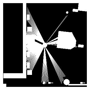
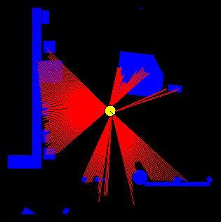
37 Sample-based Localization (sonar)

38

39

40

41

42

43

44

45

46

47

48

49

50

51

52

53

54

55

56

57

58 Using Ceiling Maps for Localization [Dellaert et al. 99]

59 Ceiling Light Localization

60 Vision-based Localization z P(z ) h()

61 Under a Light Measurement z: P(z ):

62 Net to a Light Measurement z: P(z ):

63 Elsewhere Measurement z: P(z ):

64 Sample-based Localization Demos

65 Localization Algorithms - Comparison Kalman filter Multi-hypothesis tracing Topological maps Grid-based (fied/variable) Particle filter Sensors Gaussian Gaussian Features Non-Gaussian Non-Gaussian Posterior Gaussian Multi-modal Piecewise constant Piecewise constant Samples Efficiency (memory) /+ +/++ Efficiency (time) o/+ +/++ Implementation + o + +/o ++ Accuracy /++ ++ Robustness /++ Global localization No Yes Yes Yes Yes

66 Bayes Filters for Robot Localization Grid fied/variable resolution Topological Kalman filter Etended / unscented Kalman filter Piecewise constant approimation Arbitrary posteriors Non-linear dynamics/observations Optimal, converges to true posterior Eponential in state dimensions Global localization Abstract state space Arbitrary, discrete posteriors Abstract dynamics/observations One-dimensional graph Global localization First and second moment Linear dynamics/observations Optimal (linear, Gaussian) Quadratic in state dimension Position tracing First and second moment Non-linear dynamics/observ. Not optimal (linear appro.) Quadratic in state dimension Position tracing Particle filter Sample-based approimation Arbitrary posteriors Non-linear dynamics/observations Optimal, converges to true posterior Eponential in state dimensions Global localization Multi-hypothesis tracing (EKF) Multi-modal Gaussian Non-linear dynamics/observations Not optimal (linear appro.) Polynomial in state dimension Global localization Discrete Bayes filters Continuous

67 Some Maps

68 Problems in Mapping Sensor interpretation How do we etract relevant information from raw sensor data? How do we represent and integrate this information over time? Do we map for the purpose of localization or do we map for human consumption (dense vs sparse)? Robot locations have to be nown How can we estimate them during mapping?

69 Occupancy Grid Maps Introduced by Moravec and Elfes in 1985 Represent environment by a grid. Estimate the probability that a location is occupied by an obstacle. Key assumptions Occupancy of individual cells is independent Bel(m t ) = P(m t (1: ), y(1: )) Õ,y = Bel(m t [ y] (1: ), y(1: )) Robot positions (1:) are nown!

70 The Basic Intuition A ray that flies through an area of space indicates that the space is probably free A ray where that reflects at a point indicates something there Otherwise, we don t now

71 One Idea: Simple Counting For every cell count hits(,y): number of cases where a beam ended at <,y> misses(,y): number of cases where a beam passed through <,y> Bel( m [ y] ) = hits(, y) hits(, y) + misses(, y) Assumption: P(occupied(,y)) = P(reflects(,y)) Many cases where this is not a good approimation e.g. sonar reflection model

72 Updating Occupancy Grid Maps Note that the following also can be derived: P(Øm [y] (1: ), y(1: )) = P(Øm [y] y(), ())P(y() ())P(Øm [y] (1: - 1), y(1: - 1)) Now, consider the odds ratio: O(m [ y] (1: ), y(1: )) = P( ) Odds( ) 1 P( ) P( ) P( ) ho(m [y] y(), ())O(m [ y] (1: - 1), y(1: - 1)) inverse sensor model Prior odds

73 Updating Occupancy Grid Maps Typically updated using inverse sensor model and log odds ratio (log ab = log a + log b) log O( m (1: ), y(1: )) log O( m ( ), y( )) log O( m (1: 1), y(1: 1)) logh and then recover the probability with P( ) 1 1 Odds( ) 1 P( m (1: ), y(1: )) 1 P( m ( ), y( )) h 1 P( m (1: 1), y(1: 1) 1 ( ( ), ( ) 1 ( (1: 1), (1: 1) P m y h P m y 1

74 The Inverse Sensor Model The probability a cell is occupied given observation and localization P( m ( ), y( )) Assume that all cells are independent l P ( m) P( ) then specify P( m l ( ), y( )), which is the probability of cell m l is occupied given the measurement y() in position () m l

75 Learning Inverse Sensor Model Learn probabilities with neural networ. Consider four beams simultaneously. [Thrun 98]

76 Occupancy Grid Algorithm Algorithm Occupancy_grid( 1:, y 1:, P 0 (m) ): 1. P m = P 0 (m) 2. for i=1 to ) ( ), ( ( )) ( ), ( ( 1 1 m m m P P y m P y m P P h h

77 Occupancy Grids: From scans to maps

78 Tech Museum, San Jose CAD map occupancy grid map

79 Concurrent Mapping and Localization Chicen-and-egg problem Mapping with nown poses is simple Localization with nown map is simple But in combination the problem is hard! 70 m

80 Mapping with Epectation Maimization Idea: Maimum lielihood with unnown data association. Bel(m, ()) º P((1: ), m u(0 : -1), y(1: )) Bel(m, ()) = h p(y() m, ()) ò p(() ( -1),u( -1))Bel(m, ( -1)) d t-1 Tae this apart: first estimate location given map, then estimate map given location EM: Maimize log-lielihood by iterating E-step: M-step: Q[(1: ) m [] ] = E m [ ][log p((1: ) m [],u(0 : -1), y(1: ))] [ +1] m = argma m Localization (bi-directional) Q [(1: ) m [] ] Mapping with nown poses

81 EM Mapping, Eample (width 45 m)

82 CSIRO

83 SLAM Idea: Given the true trajectory of the robot, all landmar detections are independent. P((1:),m u(0:-1),y(1:)) = P(m (1:), y(1:), u(0:-1)) P((1:) y(1:) u(0:-1)) = P(m (1:),y(1:)) P((1:) y(1:),u(0:-1)) The first term is easy (mapping given location and data) The second term is easy (predict location from prior data) The hard part: we now have to represent distributions on *trajectories*! We can use Rao-Blacwellised particle filters to estimate robot locations and landmar locations. (FastSLAM, Montemerlo) Update can be done efficiently (O(m log n)).

84 Sufficient Statistic A statistic is a function T(X 1,X 2, X n ) of the random samples X 1,X 2,,X n Eamples: X 1 n n i1 X i s 2 1 n 1 n X i X i1 T ma X1, X 2,..., 2 X n

85 Sufficient Statistic Given X 1,X 2,,X n, is there a small set of statistics that can contain all the information about the samples? If f q () is a probability distribution (q is parameter), then T is a sufficient statistic for q if we can factorize f q ( ) h( ) g ( T( )) If T is a sufficient statistic then it contain all the information to compute an estimate of q q Function of the statistic Not a function of q

86 Sufficient Statistic Given X 1,X 2,,X n, is there a statistic that can contain all the information about the samples? Poisson distribution: X 1,X 2,,X n are independent samples from a Poisson distribution with parameter l. Then a sufficient statistic T(X) of l is T( X ) i1 Note that T(X) does not depend on l n X i

87 Sufficient Statistic Given X 1,X 2,,X n, is there a statistic that can contain all the information about the samples? Eponential distribution: X 1,X 2,,X n are independent and eponentially distributed with epected value l. Then a sufficient statistic T(X) of l is T( X ) i1 Note that T(X) does not depend on l n X i

88 Rao-Blacwell Theorem Improve the efficiency of an estimator by taing its conditional epectation with respect to a sufficient statistic Estimator qˆ ( X ) : Is a statistic (rule) used to estimate an unobservable parameter q in a population The average of N random samples is an estimator of the population s average (i.e. height) Sufficient statistic T(X): Given T(X), the distribution of observable samples X does not depends on the unobservable parameter q Rao Blacwell estimator of q is defined by ˆ q ( X ) R E[ ˆ( q X ) T( X )] and has better mean squared error than qˆ ( X )

89 What About SLAM? Recall the Bayes filtering problem. The posterior satisfies the recursion P( z0: y1: ) hp( y z ) P( z z 1) P( z0: 1 y1: 1) 1 where z is hidden (put up with z instead of for now) That integral is often not tractable and numeric approimations with samples is often used z

90 Marginalize the State Space in Two Suppose we can divide z in two groups: and m such that P(z z -1 ) = P(m -1:, m -1 )P( -1 ) and assume that P(m 0: y 1:, 0: ) is tractable Then we can marginalize 0: from the posterior and focus on estimating P( 0: y 1: ) which is a smaller problem. Essentially we convert the problem to P( 0:, m 0: y 1: ) = P(m 0: y 1:, 0: ) P( 0: y 1: ) Optimal Filt. Particle Filt. and the posterior distribution of P( 0: y 1: ) is given P ( 0: y1: ) n P( y ) P( 1) P( 0: 1 y1: 1 The dimension of P( 0: y 1: ) is smaller than P( 0:, m 0: y 1: ) 1 )

91 Rao-Blacwellized SLAM Compute a posterior over the map and possible trajectories of the robot : map and trajectory p( 1 :, m y1:, u0: 1) measurements p( m 1 :, y1:, u0: t1) p( 1: y1:, u0: 1) mapping Localization map robot motion trajectory Begin Courtesy Dieter Fo

92 A Graphical Model of Rao-Blacwellized SLAM If we now the map Estimate localize at each step 1: If we now locations 1: Compute the map Particle filtering Each particle represent the posterior trajectory Compute the map corresponding to the particle s trajectory Particle s weight is given by the most lielihood of the most recent observation given the map 0 m u u u 0 1 t y 1 y 2 t y t Courtesy Dieter Fo

93 Rao-Blacwellized SLAM Brea it down even further if a map m consists of N individual landmars l i = N(m i, S i ) then P( 1:,m y 1:, u 0:-1 ) =P( 1: y 1:, u 0:-1 )P(m 1:,y 1:, u 0:-1 ) N (mi, Si ) Rao-Blacwellized particle filter (RBPF) maintains an individual map for each sample and updates this map based on the trajectory estimate of the sample Landmar are filtered individually and have low dimensionality If M particles with N landmars there is NM landmar filters i

94 FastSLAM Particle #1 Robot Pose, y, q Kalman Filters m 1, S 1 m 2, S 2 m N, S N Particle #2, y, q m 1, S 1 m 2, S 2 m N, S N Particle #3, y, q m 1, S 1 m 2, S 2 m N, S N Particle M, y, q m 1, S 1 m 2, S 2 m N, S N [Begin courtesy of Mie Montemerlo]

95 FastSLAM Algorithm O(MN) Sample a new robot pose for each particle = g( -1, u ) + v add this to trajectory giving 1: Update the landmar EKFs in each particle We have a ``nown (estimate) trajectory; run EKFs for each landmar Calculate an importance weight (difference between actual observation, y, and epected observation, with covariance Z) 1 1 T 1 w ep y yˆ n Yn y yˆ,, n, 2Y n, 2 Resample particle set

96 SLAM Data Association Angle increment = Inde1= [ ] Range1=[6.0000, , ,, , , ,, , , ] Inde2= [ ] Range2=[2.0254, , ,, , , ,, , , ]

97 SLAM Data Association In practice we use a variable n to associate each measurement to a landmar number (id#) For eample n 3 = 8 means that measurement at time =3, y 3, is associated with the landmar #8 How do we get this n? nˆ arg ma (,, ˆ, ˆ P y n y 1 n 1, u 1) n This is a Maimum Lielihood estimator.

98 FastSLAM Data Association In FastSLAM, each landmar is estimated with an EKF and the lielihood can be estimated from the EKF innovation Particle #1 Particle #2 Particle #3 Particle M Robot Pose, y, q, y, q, y, q, y, q Kalman Filters m 1, S 1 m 2, S 2 m N, S N m 1, S 1 m 2, S 2 m N, S N m 1, S 1 m 2, S 2 m N, S N m 1, S 1 m 2, S 2 m N, S N P( y y 1 1 1, nˆ 1, ˆ, u 1) ep ˆ n, n, 2Y 2 n, T 1 y yˆ Y y y n, If the lielihood falls below a threshold, a new landmar is added y ŷ

99 Tree of Landmars Particle #1 Particle #2 Particle #3 Particle M Robot Pose Particle, y, q #1 Particle, y, q #2 Particle, y, q #3 Particle M, y, q Robot Pose, y, q, y, q, y, q, y, q Kalman Filters m 1, S 1 m 2, S 2 m N, S N m 1, S 1 m 2, S 2 m N, S N m 1, S 1 m 2, S 2 m N, S N m 1, S 1 m 2, S 2 m N, S N Kalman Filters m 1, S 1 m 2, S 2 m N, S N m 1, S 1 m 2, S 2 m N, S N m 1, S 1 m 2, S 2 m N, S N m 1, S 1 m 2, S 2 m N, S N Robot Pose Particle, y, q #1 Particle, y, q #2 Particle, y, q #3 Particle M, y, q Kalman Filters m 1, S 1 m 2, S 2 m N, S N m 1, S 1 m 2, S 2 m N, S N m 1, S 1 m 2, S 2 m N, S N m 1, S 1 m 2, S 2 m N, S N FastSLAM compleity is log(mn) M number of particles N number of landmars When we resample (with replacement) the same particle may be duplicated several times Copying is linear in the size of the map Most of the landmars remain unchanged during a map update (only the visible landmars are updated) From Montemerlo 2003

100 Tree of Landmars Balanced binary tree with 8 landmars Use a tree of landmars that is shared between particles If the tree is balanced then accessing a landmar taes log(n) and FastSLAM runs in log(m logn) [Courtesy of Mie Montemerlo]

101 Tree of Landmars Modifying a landmar #3. Only m 3 and S 3 are modified Avoid duplicating the entire tree Create a new path from the root to landmar #3 Copy the missing pointers to the rest of the old tree Keep the old pointers so the other particles can use the old values [Courtesy of Mie Montemerlo]

102 FastSLAM: Victoria Par Results 4 m traverse 100 particles GPS ground truth Uses negative evidence to remove spurious landmars Uneven terrain [Courtesy of Mie Montemerlo]

103 FastSLAM: Victoria Par Results 100 meters away from it s true position 100 particles RMS error over 4m is ~4m [End courtesy of Mie Montemerlo]

104 Grid-Based FastSLAM (occupancy grid) 3 particles map of particle 1 map of particle 3 Each particle must carry its entire map map of particle 2 [Courtesy of Mie Montemerlo]

105 FastSLAM Eample 500 particles 28m28m Length of trajectory 491m Map resolution 10cm

106 Closing the Loop BEFORE AFTER [Newman 2005] Start at you are here (no uncertainty) When the loop is Close you are bac here Recognize a previously landmar Typically SLAM will drift, after a long drive the position and landmars will be off Once an previously located object is seen Mae the correction Propagate the correction bac Uncertainties collapse With great powers comes great responsibility Uncertainty is not a bad thing

107 Use camera images to detect landmars Single camera (mono) is similar to bearing only SLAM Two cameras (stereo) will give you depth as well Detect landmars (aa features ) in the image(s) Build an appearance vector around the landmar to describe its appearance Visual Landmars

108 Visual Landmars Etract landmars and their descriptors from two images. Then match the descriptors Landmars have a scale and orientation

109 Visual SLAM Bird s eye view of the 3D SIFT map SIFT landmars from stereo camera Disparities are indicated by lines Se, Lowe and Little 2005

110 RGBD SLAM (Red Green Blue Depth) Use camera and depth Provide a dense point cloud

111 Build dense, 3D, colored maps Lots of data so maps are usually small (small rooms or scanning objects) Use 3D data for localization Associate visual landmars to 3D coordinates RGBD SLAM

112 Mapping Algorithms - Comparison SLAM (Kalman) EM ML* FastSLAM Output Posterior ML/MAP ML/MAP Posterior Convergence Strong Wea? No Stong Local minima No Yes Yes No Real time Yes No Yes Yes Odom. Error Unbounded Unbounded Unbounded Unbounded Sensor Noise Gaussian Any Any Any # Features 10 3 >10 3 Feature uniq Yes No ~No Yes Raw data No Yes Yes No

113 Localization and Mapping Summary There are several methods for localization and mapping; two dominant are Kalman filter fast and efficient; very well understood local convergence strong assumptions Hypothesis-based methods (particle filters/monte Carlo methods) not as fast or efficient; not as well understood global convergence very wea assumptions The best methods today are hybrids use hypotheses as necessary use KF-lie techniques whenever possible The largest revolution in mapping and localization has been data: It s all in the lielihood function laser scanners have really revolutionized the trade vision is net?