Chapter 1. Summer School GEOSTAT 2014, Spatio-Temporal Geostatistics,

Transcription

1 Chapter 1 Summer School GEOSTAT 2014, Geostatistics, sum- Institute for Geoinformatics University of Muenster 1.1

2 Spatial Data From a purely statistical perspective, spatial data is multivariate data with special covariates: the coordinates. Tobler s first law of Geography states [3]: Everything is related to everything else, but near things are more related than distant things. sum- 1.2

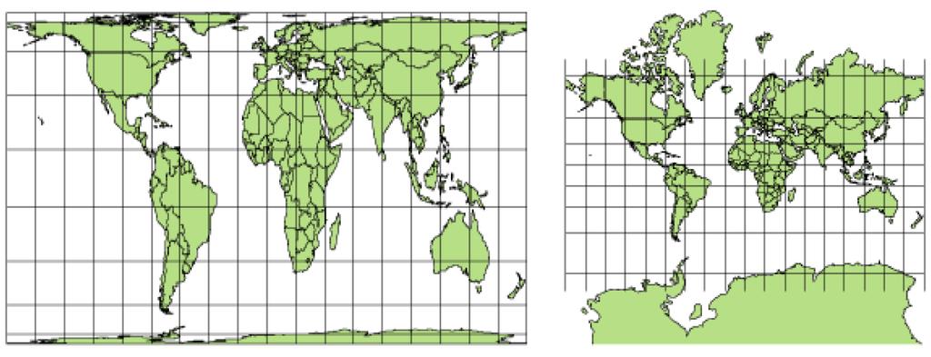
3 Coordinate Reference System We model the earth, but think in maps: locations are projected from a curved surface in 3D to flat 2D space. Be aware of geographic coordinates and different projections that maintain angles, certain distances or area. Imagine the following distances between: the Fjord of Oslo (59.85 N E) and Uppsala (59.85 N E) that are at the same latitude: Degrees: 6.88 Great Circle: 385 km Rate: 56 km/degree the intersections of the Congo river with the equator (0.00 N E) and (0.00 N, E): Degrees: 7.32 Great Circle: 814 km Rate: 111 km/degree sum- 1.3

4 Coordinate Reference System We model the earth, but think in maps: locations are projected from a curved surface in 3D to flat 2D space. Be aware of geographic coordinates and different projections that maintain angles, certain distances or area. Imagine the following distances between: the Fjord of Oslo (59.85 N E) and Uppsala (59.85 N E) that are at the same latitude: Degrees: 6.88 Great Circle: 385 km Rate: 56 km/degree the intersections of the Congo river with the equator (0.00 N E) and (0.00 N, E): Degrees: 7.32 Great Circle: 814 km Rate: 111 km/degree sum- 1.3

5 Coordinate Reference System We model the earth, but think in maps: locations are projected from a curved surface in 3D to flat 2D space. Be aware of geographic coordinates and different projections that maintain angles, certain distances or area. Imagine the following distances between: the Fjord of Oslo (59.85 N E) and Uppsala (59.85 N E) that are at the same latitude: Degrees: 6.88 Great Circle: 385 km Rate: 56 km/degree the intersections of the Congo river with the equator (0.00 N E) and (0.00 N, E): Degrees: 7.32 Great Circle: 814 km Rate: 111 km/degree sum- 1.3

6 Coordinate Reference System We model the earth, but think in maps: locations are projected from a curved surface in 3D to flat 2D space. Be aware of geographic coordinates and different projections that maintain angles, certain distances or area. Imagine the following distances between: the Fjord of Oslo (59.85 N E) and Uppsala (59.85 N E) that are at the same latitude: Degrees: 6.88 Great Circle: 385 km Rate: 56 km/degree the intersections of the Congo river with the equator (0.00 N E) and (0.00 N, E): Degrees: 7.32 Great Circle: 814 km Rate: 111 km/degree sum- 1.3

7 Coordinate Reference System We model the earth, but think in maps: locations are projected from a curved surface in 3D to flat 2D space. Be aware of geographic coordinates and different projections that maintain angles, certain distances or area. Imagine the following distances between: the Fjord of Oslo (59.85 N E) and Uppsala (59.85 N E) that are at the same latitude: Degrees: 6.88 Great Circle: 385 km Rate: 56 km/degree the intersections of the Congo river with the equator (0.00 N E) and (0.00 N, E): Degrees: 7.32 Great Circle: 814 km Rate: 111 km/degree sum- 1.3

8 Coordinate Reference System We model the earth, but think in maps: locations are projected from a curved surface in 3D to flat 2D space. Be aware of geographic coordinates and different projections that maintain angles, certain distances or area. Imagine the following distances between: the Fjord of Oslo (59.85 N E) and Uppsala (59.85 N E) that are at the same latitude: Degrees: 6.88 Great Circle: 385 km Rate: 56 km/degree the intersections of the Congo river with the equator (0.00 N E) and (0.00 N, E): Degrees: 7.32 Great Circle: 814 km Rate: 111 km/degree sum- 1.3

9 Coordinate Reference System We model the earth, but think in maps: locations are projected from a curved surface in 3D to flat 2D space. Be aware of geographic coordinates and different projections that maintain angles, certain distances or area. Imagine the following distances between: the Fjord of Oslo (59.85 N E) and Uppsala (59.85 N E) that are at the same latitude: Degrees: 6.88 Great Circle: 385 km Rate: 56 km/degree the intersections of the Congo river with the equator (0.00 N E) and (0.00 N, E): Degrees: 7.32 Great Circle: 814 km Rate: 111 km/degree sum- 1.3

10 Coordinate Reference System We model the earth, but think in maps: locations are projected from a curved surface in 3D to flat 2D space. Be aware of geographic coordinates and different projections that maintain angles, certain distances or area. Imagine the following distances between: the Fjord of Oslo (59.85 N E) and Uppsala (59.85 N E) that are at the same latitude: Degrees: 6.88 Great Circle: 385 km Rate: 56 km/degree the intersections of the Congo river with the equator (0.00 N E) and (0.00 N, E): Degrees: 7.32 Great Circle: 814 km Rate: 111 km/degree sum- 1.3

11 CRS identifier To distinguish different projections, a well prepared data set comes with its coordinate reference system (CRS) as metadata. These are often encoded as EPSG-codes (by the European Petroleum Survey Group) proj4string They define how the reference surface (sphere, ellipsoid) is fixed to the real world (called the datum) and how the projection (surface in 3D to 2D plane) is made. sum- 1.4

12 Projection sum- 1.5

13 Fields Fields are understood as continuously spreading over space and/or time (e.g. temperature recordings) and typically observed at a set of distinct locations for a series of time steps. Fields are typically illustrated as interpolated maps and modelled as a realisation of a spatial/ random field. obs. zinc concentrations interpol. zinc concentrations sum- 1.6

14 Stationarity and Isotropy stationarity The process looks the same at each location (e.g. mean and variance do not change from east to west) isotropy The dependence between locations is determined only by their separating distance neglecting the direction (e.g. locations 2 km apart along the north-south axis are as correlated as stations 2 km apart along the east-west axis) Some tricks exist to weaken these assumptions (e.g. rotating and rescaling coordinates). sum- 1.7

15 Variograms I The dependence across space of a random field Z is assessed using a variogram γ: γ(h) = 1 2 E( Z(s) Z(s + h) ) 2 the estimator looks like ˆγ(h) = 1 2 N h (i,j) N h ( Z(si ) Z(s j ) ) 2 while N h = {(i, j) : h ɛ s i s j h + ɛ} sum- 1.8

16 Variograms II The sample variogram is obtained through vgmmeuse <- variogram(zinc~1, meuse) semivariance sum distance 1.9

17 Variograms III And a theoretical variogram model can be fitted > head(vgm()) short long 1 Nug Nug (nugget) 2 Exp Exp (exponential) 3 Sph Sph (spherical) 4 Gau Gau (gaussian) 5 Exc Exclass (Exponential class) 6 Mat Mat (Matern) > vgmmodelmeuse <- fit.variogram(vgmmeuse, vgm(0.6, "Sph", 1000, 0.1)) vgmmodelmeuse model psill range 1 Nug Sph sum- 1.10

18 Variograms IV semivariance sum distance 1.11

19 I Certain variogram models can be used to parametrize a covariance matrix for a Gaussian random field over a finite set of locations s 1,..., s n : Z Gau ( µ, Σ ) while Σ = (σ 2 ij ) ij and σ 2 ij = σ2 γ( s i s j ), 1 i, j n with σ 2 = Var ( Z(s) ), µ = (µ 1,..., µ n ). Predictions can be made using matrix inversion and matrix multiplications. sum- 1.12

20 II krige(zinc~1, meuse, meuse.grid, model=vgmmodelmeuse) obs. zinc concentrations kriged zinc concentrations sum- 1.13

21 III The model quantifies how uncertain it is about the estimates through the kriging variance: kriged zinc concentrations kriging variance sum

22 Overview of kriging types simple kriging the mean value is known ordinary kriging prediction based on coordinates universal kriging prediction based on coordinates and additional regressors (distance to the river) co-kriging the cross-variogram between two variables is as well exploit (zinc and lead) sum- 1.15

23 Overview of kriging types simple kriging the mean value is known ordinary kriging prediction based on coordinates universal kriging prediction based on coordinates and additional regressors (distance to the river) co-kriging the cross-variogram between two variables is as well exploit (zinc and lead) sum- 1.15

24 Overview of kriging types simple kriging the mean value is known ordinary kriging prediction based on coordinates universal kriging prediction based on coordinates and additional regressors (distance to the river) co-kriging the cross-variogram between two variables is as well exploit (zinc and lead) sum- 1.15

25 Overview of kriging types simple kriging the mean value is known ordinary kriging prediction based on coordinates universal kriging prediction based on coordinates and additional regressors (distance to the river) co-kriging the cross-variogram between two variables is as well exploit (zinc and lead) sum- 1.15

26 Data S T works as a data structure, but modelling needs to consider special properties of the product of space and time. direction Today s values influence tomorrow, but will not take effect on yesterday s values. anisotropy What is the equivalent in terms of dependence of 1 m separation in seconds or minutes? The easiest way to think of data is as time slices - but this neglects the temporal dependence. After modelling temporal trend or periodicities, the residuals might be modelled as a random field. sum- 1.16

27 Almost approaches slice wise the easiest adoption is to do interpolation per slice fitting a variogram model for each time slice pooled the variogram is fitted based on all data and is used to predict each time slice separately with the same model evolving models mix the both extremes such that the variogram model adopts to the daily situation (e.g. in terms of overall variability, the sill) but range and the nugget/sill ratio depend on larger data samples. sum- 1.17

28 Almost approaches slice wise the easiest adoption is to do interpolation per slice fitting a variogram model for each time slice pooled the variogram is fitted based on all data and is used to predict each time slice separately with the same model evolving models mix the both extremes such that the variogram model adopts to the daily situation (e.g. in terms of overall variability, the sill) but range and the nugget/sill ratio depend on larger data samples. sum- 1.17

29 Almost approaches slice wise the easiest adoption is to do interpolation per slice fitting a variogram model for each time slice pooled the variogram is fitted based on all data and is used to predict each time slice separately with the same model evolving models mix the both extremes such that the variogram model adopts to the daily situation (e.g. in terms of overall variability, the sill) but range and the nugget/sill ratio depend on larger data samples. sum- 1.17

30 The variogram Extending the variogram to a twoplace function for random fields Z(s, t): γ(h, u) = E ( Z(s, t) Z(s + h, t + u) ) 2 at any location (s, t). And version ˆγ(h, u) = 1 2 N h,u (i,j) N h,u ( Z(si, t i ) Z(s j, t j ) ) 2 { while N h,u = (i, j) h ɛ } s s i s j h + ɛ s u ɛ t t i t j u + ɛ t sum- 1.18

31 sum Scenario We have a set of spatially spread time series of daily measurements and are asked to produce a map of means for the provided time frame. The data is provided by the EEA, the presentation is composed along the lines of [2] [0,5] (5,10] (10,15] (15,20] (20,25] (25,30]

32 variogram surface The idea is the same as in the spatial case: binning of locations according to their separating distance. In the case, distances are pairs of spatial and temporal distance yielding a variogram surface, not a single line. empvgm <- variogramst(pm10~1, ger_june, tlags=0:4, cutoff=500e3) # rescalig of distances empvgm$dist <- empvgm$dist/1000 empvgm$spacelag <- empvgm$spacelag/1000 # wireframe: plot(empvgm, wireframe=t, scales=list(arrows=f), col.regions=bpy.colors(),zlab=list(rot=90),zlim=c(0,20)) sum- # levelplot: plot(empvgm) 1.20

33 variogram surface - wireframe 18 gamma sum time lag (days) distance

34 variogram surface - levelplot 18 4 time lag (days) sum distance 1.22

35 kriging The kriging follows the natural idea of extending the 2-dimensional geographic space into a 3-dimensional one. In order to achieve an isotropic space, the temporal domain has to be rescaled to match the spatial one ( anisotropy correction κ). All spatial, temporal and sptio-temporal distances are treated equally resulting in a joint covariance model C j : The variogram evaluates to C m (h, u) = C j ( h 2 + (κ u) 2) sum- γ m (h, u) = γ j ( h 2 + (κ u) 2 ) where γ j is any known variogram including some nugget effect. 1.23

36 kriging in R Model <- vgmst("", joint=vgm(0.8,"exp", 150, 0.2), stani=100) Fit <- fit.stvariogram(empvgm,model, lower=c(0,10,0,10)) attr(fit,"optim.output")$value > plot(empvgm, Fit) predmetric <- krigest(pm10~1, ger_june, STF(ger_gridded,tgrd), Fit) sum- 1.24

37 variogram surface sample time lag (days) sum distance 1.25

38 kriged map for day 15 - model day sum

39 covariance models In space and under the assumptions of isotropy and stationarity, the covariance is a function C(h) of the separating distance h between two locations. A covariance function is thought of as a function of a spatial and a temporal distance C(h, t). A covariance function is assumed to fulfill C sep (h, u) = C s (h)c t (u). This is in general a rather strong simplification. Its variogram is given by γ sep (h, u) = nug 1 h>0,u>0 +sill (γ s (h)+γ t (u) γ s (h)γ t (u) ) sum- where γ s and γ t are spatial and temporal variograms without nugget effect and a sill of 1. The overall nugget and sill parameters are denoted by nug and sill respectively. 1.27

40 covariance model in R sepmodel <- vgmst("", space=vgm(0.8,"exp", 150, 0.2), time =vgm(0.7,"exp", 6, 0.3), sill=18) sepfit <- fit.stvariogram(empvgm,sepmodel, lower=c(10,0,1,0,0)) attr(sepfit,"optim.output")$value > plot(empvgm, sepfit) predsep <- krigest(pm10~1, ger_june, STF(ger_gridded,tgrd), sepfit) sum- 1.28

41 variogram surface of the model sample time lag (days) sum distance 1.29

42 kriged map for day 15 - seperable covariance model day sum

43 covariance model The product sum covariance model extends the simplifying assumption of the covariance model to [1]: C ps (h, u) = k 1 C s (h) + k 2 C t (u) + k 3 C s (h)c t (u) with k 1 > 0, k 2 0 and k 3 0 to fulfil the positive-definite condition. The corresponding variogram can be written as γ ps (h, u) = nug 1 h>0,u>0 + γ s (h) + γ t (u) kγ s (h)γ t (u) where γ s and γ t are spatial and temporal variograms without nugget effect and in general different sills. The parameter k needs to fulfil 0 < k 1/(max(sill s, sill t )) to let γ ps be a valid model. The overall nugget is denoted by nug. sum- 1.31

44 covariance model in R empvgm$dist <- empvgm$dist/10 empvgm$spacelag <- empvgm$spacelag/10 psmodel <- vgmst("productsum", space=vgm(11,"exp", 2), time =vgm(5,"sph", 6), sill=16, nugget=5) psfit <- fit.stvariogram(empvgm,psmodel) attr(psfit,"optim.output")$value > plot(empvgm, psfit) predps <- krigest(pm10~1, ger_june, STF(ger_gridded,tgrd), psfit) sum- 1.32

45 variogram of the model sample productsum 18 time lag (days) sum distance 1.33

46 kriged map for day 15 - covariance model day sum

47 sum- covariance model The sum- covariance model is given by: C sm (h, u) = C s (h) + C t (u) + C j ( h 2 + (κ u) 2) Originally, this model allows for spatial, temporal and joint nugget effects, a simplified version may allow only for a joint nugget. The non-simplified variogram is given by γ sm (h, u) = γ s (h) + γ t (u) + γ j ( h 2 + (κ u) 2 ) where γ s, γ t and γ j are spatial, temporal and joint variograms with a separate nugget-effect. sum- 1.35

48 sum- covariance model in R empvgm$dist <- empvgm$dist/10 empvgm$spacelag <- empvgm$spacelag/10 summetricmodel <- vgmst("summetric", space=vgm(5,"exp",10,2), time =vgm(5,"exp", 6,2), joint=vgm(5,"exp",10,2), stani=10) summetricfit <- fit.stvariogram(empvgm,summetricmodel, lower=c(0,1,0,0,1,0,0)) attr(summetricfit,"optim.output")$value > plot(empvgm, summetricfit) sum- predsummetric <- krigest(pm10~1, ger_june, STF(ger_gridded,tgrd), summetricfit) 1.36

49 variogram of the sum- model sample summetric time lag (days) sum distance 1.37

50 kriged map for day 15 - covariance model day sum

51 variogram of all models sample 20 productsum summetric sum

52 kriged map for 10 days sum

53 over time In the above scenario and with the presented methods, it is hard to get an uncertainty estimate of the temporally averaged value. Block kriging, with blocks over time, is one way to get such estimates. However, one has to decide on a model beforehand. Here, we will use the model again. Block kriging does not provide estimates for single locations but for areas or volumes. It has the property of providing the correct kriging variance for the block estimate that is typically lower due to the larger area. sum- 1.41

54 monthly mean concentration - block kriged sum- 1.42

55 variance sum- 1.43

56 kriging variance day 15 sum- 1.44

57 in R - workaround tmp_pred <- data.frame(cbind(ger_gridded@coords,15*tmpscale)) colnames(tmp_pred) <- c("x","y","t") coordinates(tmp_pred) <- ~x+y+t blockkrige <- krige(pm10~1, air3d[as.vector(!is.na(air3d@data)),], newdata=tmp_pred, model=model3d, block=c(1,1,15*tmpscale)) ger_grid_time@sp@data <- blockkrige@data sum- 1.45

58 local kriging Purely spatial kriging allows to select the n-nearest neighbours and use only these for prediction. What does nearest mean in a context? The idea is to select the most valuable locations, i.e. the strongest correlated ones. Simply set the argument nmax and a local neighbourhood of the most correlated values is selected from a larger neighbourhood. sum- 1.46

59 I [1] S. De Iaco, D.E. Myers, and D. Posa. Space-time analysis using a general model. Statistics & Probability Letters, 52(1):21 28, [2], Lydia E. Gerharz, and Edzer J. Pebesma. Spatio-temporal analysis and interpolation of PM10 measurements in Europe. Technical report, ETC/ACM, [3] W. R. Tobler. A computer movie simulating urban growth in the detroit region. Economic Geography, 46: , sum- 1.47