ESTIMATING THE MEAN LEVEL OF FINE PARTICULATE MATTER: AN APPLICATION OF SPATIAL STATISTICS

Transcription

1 ESTIMATING THE MEAN LEVEL OF FINE PARTICULATE MATTER: AN APPLICATION OF SPATIAL STATISTICS Richard L. Smith Department of Statistics and Operations Research University of North Carolina Chapel Hill, N.C., U.S.A. Boston University April

2 I. CONSTRUCTING A MAP OF ANNUAL AVERAGES OF FINE PARTICULATE MATTER Based on Smith, Kolenikov and Cox, Journal of Geophysical Research, II. SOME THEORETICAL ASPECTS OF BAYESIAN SPATIAL PREDICTION Work currently in progress, with Z. Zhu, J. Ibrahim and E. Shameldin (UNC). 2

3 Background to Part I A new set of air pollution standards, first proposed in 1997, is finally being implemented by the U.S. Environmental Protection Agency (EPA). One of the requirements is that the mean level of fine particulate matter (PM 2.5 ) at any location should be no more than 15 µg/m 3. A network of several hundred monitors has been set up to assess this. The present study is based on 1999 data for a small portion of this network, 74 monitors in North Carolina, South Carolina and Georgia. We converted the raw values to weekly averages, but even so more than 1 4 of the data are missing. The EPA also recorded a land-use variable, classified as one of five types of land-use: agricultural (A), commercial (C), forest (F), industrial (I) and residential (R). 3

4 4

5 Exploratory data analysis The first issue considered is whether to make any transformation, such as square roots or logarithms, of the raw PM 2.5 values. We show a plot of sample variance against sample mean, across all 74 stations, for each of three transformations, (a) no transformation, (b) square root transformation, (c) logarithmic transformation. On the basis that (b) is the closest fit to a constant-variance model, the rest of the analysis is based on the square root of PM 2.5 as a variance-stabilizing transformation. 5

6 6

7 The time trend The time trend was estimated both as a B-spline smooth curve and (more simply) by using a weekly indicator variable to represent the overall mean level for that week. Fig. (a) shows both versions of the fitted time trend, with all data points superimposed. Also shown are the same fitted time trend curves, but with different portions of the data superimposed, (b) (d) corresponding to each of the three states, (e) (i) corresponding to each of the five land-use variables. The results show a significant discrepancy between states, with Georgia values generally higher than the overall mean, while the land-use variables show significant variations in the directions one would expect. 7

8 8

9 These comparisons suggest the model y xt = w t + ψ x + θ x + η xt (1) in which y xt is the square root of PM 2.5 in location x in week t, w t is a week effect, ψ x is the spatial mean at location x (in practice, estimated through a thin-plate spline representation), θ x is a land-use effect corresponding to the land-use as site x, and η xt is a random error. So far we have ignored temporal and spatial correlations among the η xt, but we consider these next. 9

10 Spatial and temporal dependence Take residuals from preceding linear regression. Plots of autocorrelations suggest series are uncorrelated in time but not in space. 10

11 11

12 We show variograms of residuals from simple linear regression, where a number of subsets of the data (classified by state and also by season) have been identified to look for comparability of the estimated variogram among different subsets of data. Key points are Substantial inhomogeneity among subgroups despite initial variance stabilization Does not seem to follow standard nugget-range-sill shape 12

13 13

14 We fit the power law variogram { 0 if h = 0, γ(h) = θ 0 + θ 1 h λ if h > 0, where θ 0 > 0, θ 1 > 0, 0 λ < 2. (2) 14

15 To fit this model by maximum likelihood, we need the concept of generalized covariances, introduced by Matheron (1973). For modern references see Cressie (1993), Chilès and Delfiner (1999) or Stein (1999). In the present context the key formula is the following: for an intrinsically stationary process defined by a semivariogram γ, Cov x ν x η x,t, x κ x η x,t = ν x κ x G( x x ), x x provided x ν x = x κ x = 0. Here G is known as the generalized covariance function: however for an intrinsically stationary process, it suffices to take G = γ. 15

16 Practical implementation: In (1), replace each y xt by yxt = y xt n 1 t x y x t where the second sum is over all x values available in week t; n t is the number of such x values in a given week. With some further simplifications we replace (1) by where y xt = ψ x + θ x + η xt (3) Cov{η x,t, η x,t } = 1 n t + 1 n t 1 n 2 t x 1 γ( x x 1 ) x 1 γ( x x 1 ) γ( x x ) x 1 x 2 γ( x 1 x 2 ). (4) The model defined by (2) (4) may now be fitted by maximum likelihood. 16

17 There are additional complications because of the missing values, which mean that n t and the fitted covariance matrix are different from week to week. The present data set is relatively small and we were still able to compute exact maximum likelihood, but some variants of the EM algorithm (Little and Rubin 1987, McLachlan and Krishnan 1997) were also used, and remain the focus of further research. 17

18 Results The model (3) was fitted to the data values from which each weekly mean had been subtracted. The residuals ηxt were assumed independent at different time points but with spatial covariances given by (4) with (2). As an example of the results, the maximum likelihood of the parameter θ 2 was 0.92 with standard error Since a linear variogram corresponds to θ 2 = 1, this shows that the spatial dependence is not significantly different from a linear variogram. 18

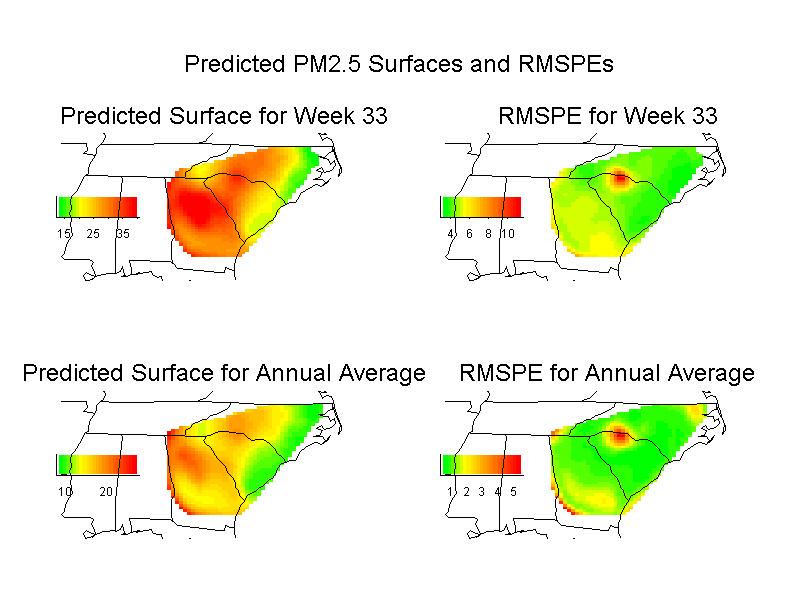
19 The fitted model was then used to construct a predicted surface, with estimated root mean squared prediction error (RMSPE), for each week of the year and also for the average over all weeks. The latter is of greatest interest in the context of EPA standards setting. 19

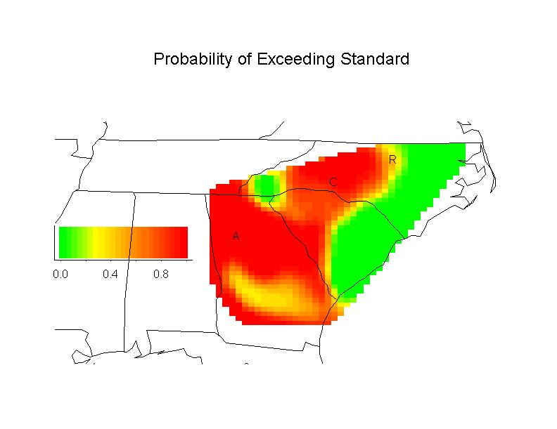
20 We show the predicted surface and RMSPE for week 33 (the week with highest average PM 2.5 ) and overall for the annual mean. WE also show shows the estimated probability that any particular location exceeds the 15 µg/m 3 annual mean standard. These maps are based on kriging the residuals ηxt in (2) and then combining them with the estimated fixed effects for ψx and θx, transforming back to the original scale of the data for the actual plots. The RMSPE values used here take into account the averaging of kriged values, but do not take account of the additional uncertainty in estimating the parameters θ 1 and θ 2. Fig. 6 is based on the assumption that (on a square root scale) the difference between the predicted and true values, scaled by the RMSPE, has a standard normal distribution. 20

21 It can be seen that substantial parts of the region, including the western portions of North and South Carolina and virtually the whole of the state of Georgia, appear to be in violation of the standard. Of the three major cities marked on the last figure, Atlanta and Charlotte are clearly in the violation zone; Raleigh is on the boundary of it. In future work, we hope to extend this analysis to other parts of the country (this will certainly involve consideration of nonstationary spatial models), to analyze more recent data, and to consider the associated network design questions. 21

22 22

23 23

24 II. SOME THEORETICAL ASPECTS OF SPATIAL PREDICTION We assume data follow a Gaussian random field with mean and covariance functions represented as functions of finite-dimensional parameters. Define the prediction problem as ( ) [( Y Xβ N x T 0 β Y 0 ), ( V w T w v 0 where Y is an n-dimensional vector of observations, Y 0 is some unobserved quantity we want to predict, X and x 0 are known regressors, and β is a p-dimensional vectors of unknown regression coefficients. For the moment, we assume V, w and v 0 are known. )] 24 (5)

25 Where notationally convienient, we also define Y = write (5) as ( Y Y 0 ) and Y N[X β, V ]. (6) 25

26 Specifying the Covariances The most common and widely used spatial models (stationary and isotropic) assume the covariance between components Y i and Y j is a function of the (scalar) distance between them, C(d ij ). For example, C θ (d) = σ exp where θ = (σ, ρ) (exponential), C θ (d) = σ exp where θ = (σ, ρ) (Gaussian), C θ (d) = σ 2 ν 1 Γ(ν) ( ( 2ν 1/2 d ρ d ρ ) ( ) 2 d ρ )ν, (7), (8) ( 2ν 1/2 ) d K ν, (9) ρ where K ν is a modified Bessel function and we have θ = (ν, σ, ρ) (Matérn). 26

27 Estimation Model of form Y N[Xβ, V (θ)] where the unknown parameters are (β, θ) and V (θ) is a known function of finite-dimensional parameters θ. Methods of estimation: 1. Curve fitting to the variogram, based on residuals from OLS regression. 2. Maximum likelihood (MLE) 3. Restricted maximum likelihood (REML) 27

28 The Main Prediction Problem Assume model (5) where the covariances V, w, v 0 are known but β is unknown. The classical formulation of universal kriging asks for a predictor Ŷ 0 = λ T Y that minimizes σ 2 0 = E { (Y 0 Ŷ 0 ) 2} subject to the unbiasedness condition E { Y 0 Ŷ 0 } = 0. The classical solution: Ŷ 0 = w T V 1 Y + (x 0 X T V 1 w) T (X T V 1 X) 1 X T V 1 Y, σ 2 0 = v 0 w T V 1 w + (x 0 X T V 1 w) T (X T V 1 X) 1 (x 0 X T V 1 w). 28

29 In traditional geostatistics, the covariances are estimated in a separate estimation step assuming a parametric model such as one of (7) (9). However, the estimation is then ignored in applying universal kriging. This is potentially a problem, because we would expect the prediction variance to be larger if we took into account the uncertainty in estimating θ. Bayesian methods provide a potential way round this difficulty, because in a Bayesian analysis we integrate out the predictive density with respect to the posterior density of all the unknown parameters. This is straightforward to implement via MCMC and is starting to be implemented in some widely available packages (GeoR, GeoBugs). However, this raises the question of what are the sampling properties of such procedures. The aim of the present research is to investigate such questions via asymptotic theory. 29

30 Bayesian Reformulation of Universal Kriging Assume the model (5) or equivalently (6). Suppose β (the only unknown parameter, for the moment) has a prior density which is assumed uniform across R p. The Bayesian predictive density of Y 0 given Y is then p(y 0 Y ) = f(y β)dβ f(y β)dβ. (10) This may be rewritten in the form p(y 0 Y ) = (2π) 1/2 V 1/2 X T V 1 X 1/2 e G 2 /2 V 1/2 X T V 1 X 1/2. (11) e G2 /2 where G 2 = Y T {V 1 V 1 X(X T V 1 X) 1 X T V 1 }Y is the generalized residual sum of squares for the vector Y and G 2 is the same thing for the vector Y. 30

31 However, with some algebraic manipulation we can show, V X T V 1 X V X T V 1 X = σ 2 0, (12) G 2 = G 2 + (Y 0 Ŷ 0 ) 2. (13) The Bayesian predictive density then becomes p(y 0 Y ) = 1 ( ) 2 Y0 2πσ0 2 exp 1 Ŷ 0 (14) 2 σ 0 Thus, in the case where β is the only unknown, we have rederived universal kriging as a Bayesian predictor. However, because of the usual (frequentist) derivation of universal kriging, it follows that in this case, Bayesian procedures have exact frequentist properties, e.g. a Bayesian 95% prediction interval for Y 0 will indeed cover the true Y 0 in 95% of repeated samples. σ

32 Now consider the case where θ is also unknown. We assume θ has a prior density π(θ), independent of β. The Bayesian predictive density of Y 0 given Y is now p(y 0 Y ) = f(y β, θ)π(θ)dβdθ f(y β, θ)π(θ)dβdθ = (2π) 1/2 V 1/2 X T V 1 X 1/2 e G 2 /2 π(θ)dθ V 1/2 X T V 1 X 1/2 e G2 /2. π(θ)dθ Using (12) and (13), p(y 0 Y ) may be rewritten V 1/2 X T V 1 X 1/2 e G2 /2 (2πσ 2 0 ) 1/2 exp V 1/2 X T V 1 X 1/2 e G2 /2 π(θ)dθ { ( ) } 2 1 Y0 Ŷ 0 2 σ 0 π(θ)dθ. (15) 32

33 (15) is of the form p(y 0 Y ) = ψ = e l n (θ) ψ(θ)π(θ)dθ e l n (θ) π(θ)dθ (16) where e l n(θ) is the restricted likelihood of θ given the data Y and ψ(θ) = (2πσ 2 0 ) 1/2 exp { ( ) } 2 1 Y0 Ŷ 0 2 σ 0 is the predictive density we are trying to evaluate, written as a function of θ. The function e l n(θ) may be alternatively derived from purely frequentist considerations as the likelihood of a set of orthogonal contrasts in the original X space. However, it has been known since Harville (1974) that this is equivalent to the Bayesian derivation as an integrated likelihood with respect to β. The best regarded (frequentist) estimator of θ is the so-called restricted maximum likelihood or REML estimator ˆθ which maximizes l n (θ). 33

34 Solution of (16): Use Laplace approximation. First, some notation. Let U i = l n(θ) θ i, U ij = 2 l n (θ) θ i θ j, U ijk = 3 l n (θ) θ i θ j θ k, where θ i, θ j... denote components of the vector θ. Suppose inverse of {U ij } matrix has entries {U ij }. 34

35 We shall introduce other quantities such as Q(θ) and ψ(θ) that are functions of θ, and where needed, we use suffixes to denote partial differentiation, for example Q i = Q/ θ i, ψ ij = 2 ψ/ θ i θ j. All these quantities are evaluated at the true θ unless denoted otherwise. The maximum likelihood estimator (MLE) is denoted ˆθ with components ˆθ i. The MLE of ψ is ˆψ = ψ(ˆθ). Any expression with a hat on it, such as Û ijk, means that it is to be evaluated at the MLE ˆθ rather than the true value θ. 35

36 Using summation convention, define D = 1 2 U ijku ik U jl ψ l 1 2 (ψ ij + 2ψ i Q j )U ij (17) and let ˆD denote the same expression where all terms have hats. With these conventions, an application of Laplace s integral formula leads to accurate to O p (n 1 ). ψ = ˆψ + ˆD, (18) Apply to predictive inference: recast as predictive distribution function (rather than density) so ( y λ T ) Y ψ(y; Y, θ) = Φ σ 0 where Ŷ 0 = λ T Y and σ0 2 universal kriging. are the point prediction and MSPE under 36

37 ψ (y; Y, θ) = 1 [ Φ y λ T Y, σ 0 σ 0 ψ (y; Y, θ) = 1 [ σ0 2 Φ y λ T ] Y, σ 0 ψ i (y; Y, θ) = { y λ T } [ Y θ i Φ y λ T ] Y, σ 0 σ 0 { ψ ij (y; Y, θ) = 2 y λ T } [ Y θ i θ j Φ y λ T Y + θ i σ 0 { y λ T Y σ 0 ] } Φ [ y λ T Y σ 0 θ j ]. σ 0 { y λ T Y σ 0 ] } 37

38 Define a maximum likelihood or plug-in formula by ˆψ(y; Y ) = ψ(y; Y, ˆθ). The Bayesian predictor, ψ(y; Y ), is defined by (16) in which ψ(θ) is replaced by ψ(y; Y, θ). Equations (17) and (18) so far give an approximation to ψ(y; Y ), accurate to O p (n 1 ). Now let us consider the corresponding quantile problem. Suppose we are interested in determining the value y P for which the event Y 0 y has conditional probability P, given Y. Here P is a fixed constant between 0 and 1. We can define two natural estimators by inverting the maximum likelihood and Bayesian predictive distribution functions. Specifically, ŷ P satisfies ˆψ(ŷ P ; Y ) = P and ỹ P satisfies ψ(ỹ P ; Y ) = P. In the case P 1 = α/2, P 2 = 1 α/2, the intervals (ŷ P1, ŷ P2 ) and (ỹ P1, ỹ P2 ) are natural candidates for a 100(1 α)% prediction interval for y 0. One of the questions of interest is what is the true coverage probability of either of these intervals in repeated sampling it would be ideal if the coverage probability was exactly 1 α. 38

39 For ŷ P, we simply substitute maximum likelihood estimator for unknown parameters throughout, and obtain the exact solution ŷ P = ˆλ T Y + ˆσ 0 Φ 1 (P ) (19) where Φ 1 ( ) is the inverse standard normal distribution function. For ỹ P, a Taylor expansion based on (18) suggests the approximation ỹ P = ŷ P ˆD(ŷ P ) ˆψ (ŷ P ; Y ). (20) Here ˆD(ŷ P ) is defined by (17) where we evaluate all functions of θ at θ = ˆθ and, in addition, evaluate the function ψ(y; Y, θ) at y = ŷ P ; we also define ˆψ (y; Y ) = ψ (y; Y, ˆθ). Since ˆD = O p (n 1 ), it follows that (20) is also accurate to O p (n 1 ). 39

40 Future Work 1. Investigate the computational properties of this procedure as an alternative to MCMC. 2. Bias in coverage probability how far do the true coverage probabilities of either the likelihood or Bayesian prediction intervals differ from their nominal levels? 3. Design of a network: a reasonable criterion for design of a monitoring network might be to do it to minimize the expected length of a Bayesian prediction interval (of some quantity of particular interest, such as the statewide average of particular matter). The present approach allows for a combination of estimative and predictive criteria which is in line with recent research in this field (Zhu, 2002, U. Chicago thesis). 40