Lecture 9: Introduction to Kriging

Transcription

1 Lecture 9: Introduction to Kriging Math 586 Beginning remarks Kriging is a commonly used method of interpolation (prediction) for spatial data. The data are a set of observations of some variable(s) of interest, with some spatial correlation present. Usually, the result of kriging is the expected value ( kriging mean ) and variance ( kriging variance ) computed for every point within a region. Practically, this is done on a fine enough grid. Illustration: suppose we observe some variable Z along 1-dim space (X). There are 5 measurements made. We might ask ourselves, knowing the probabilistic behavior of the random field being observed, what are possible trajectories (realizations) of the random field, that agree with the data? This is answered by conditional simulation. In Fig. 1, you see two sets of 5 conditional simula- Conditional simulation: 5 realizations Other 5 realizations: higher krig. variance Z Z X X Figure 1: Conditional simulations, data given by dots tions for the same data. The one on the left is for one value of σ 2 = variance 1

2 of the random field, the one on the right is for another, higher, value. All the realizations are faithful to the data, but also faithful to the statistical model for the random field (i.e. mean and variogram) that we selected. Kriging mean for every location can be thought of as the average of the whole ensemble of possible realizations, conditioned on data. Kriging variance is the variance of that ensemble. (The ensemble is of course infinite, we only show 5 of its representatives.) You may see that the trajectories tend to diverge away from the observed data, that is, the kriging variance increases. Also, for the random field with higher variance (the one on the right in Fig. 1) We will observe similar qualitative behavior frequently in the future. Simple kriging (SK) Let us observe some stationary (WSS) random field V (x) at some points x j, j = 1,..., n. First, assume that the mean m and covariance function C( ) of this process are known. The case of prediction with the known mean is often called simple kriging. In order to better understand what happens and to devise an extendable approach, let s attack the question by directly trying to minimize MSE. We will seek an estimate ˆV 0 of the value of V at the point x 0. For simplicity, denote V j := V (x j ). Also, denote C(i, j) = Cov(V i, V j ). We may assume that the mean m = 0. Otherwise, subtract m from all of the V j values, estimate V 0, then add the mean back. Search for the estimate of the form ˆV 0 = n λ j V j, j=1 under the assumption of 0 mean, it is automatically unbiased. (Why?) We will find the kriging weights λ j that minimize MSE: [ ( MSE = E V 0 ) ] 2 λ j V j = V ar (V 0 ) λ j V j = (Why?) = V ar(v 0 ) 2 λ j Cov(V 0, V j ) + λ j λ i Cov(V i, V j ) That is, MSE = C(0, 0) 2 λ j C(0, j) + λ j λ i C(i, j) (1) 2

3 where C(i, j) = C V (x i x j ) might be interpreted as the elements of covariance matrix C. Note that the values C(0, j) depend on the location x 0. To minimize MSE, we take the derivatives with respect to λ k and equate to 0: MSE λ k = 2C(0, k) + 2λ k C(k, k) + 2 j k λ j C(k, j) = 0, k = 1,..., n That is, solve the system of equations 1 n λ j C(k, j) = C(0, k), k = 1,..., n (2) j=1 In matrix form, the above equations look like Cλ = b same as λ = C 1 b (3) If we denote the covariance matrix of the vector (V 0, V 1,..., V n ) as Σ, then [ ] σ 2 Σ = 0 b and MSE= σsk 2 = C(0, 0) 2λ b+λ Cλ = C(0, 0) λ b b C Now compare the equation (3) with the formula for conditional mean in Lecture 6, p. 4. It turns out that the above minimization argument is directly related to the BLUE theory for multivariate Normal! To avoid ambiguity, we will sometimes denote the optimal kriging weights λ SK. From the equations (1) and (2), the optimal kriging variance is σ 2 SK = C(0, 0) λ SK j C(0, j) (4) Compare this to the conditional variance formula from Lecture 6. What happens when you predict at one of the existing points x j? It is clear that the best choice is to just take V j, in which case the kriging variance is 0! If we use the covariance function such that C(h) C(0)σ 2 as h 0, that is, dealing with a continuous random field (no nugget!), then we should obtain lim ˆV (x0 ) = V j and σsk 2 0 x 0 x j 1 Note that we really did not use the assumption of WSS stationarity, since we allowed C(i, j) to vary with location x i. We don t have to assume a constant mean m, either, and can replace it by varying values m i, as long as these are known. 3

4 A simple case: Suppose that C(i, j) = 0, i j, only C(0, j) 0, j = 1,..., n. In this case, the kriging equations (2) are solved by λ j = σ 0 C(0, j) C(j, j) = ρ 0,j, σ j where ρ 0,j is the correlation coefficient. We obtain the prediction ˆV 0 σ 0 = ρ 0,j V j σ j That is, the weights reflect the strength of correlation. This reminds us of simple linear regression. Also, σ 2 SK = σ 2 0(1 ρ 2 0,j) where we recognize the quantity ρ 2 0,j as coefficient of determination R 2! (Question: why ρ 2 0,j 1?) Summary: Kriging is an exact interpolator (it preserves the observations) when there s no nugget effect. Kriging weights λ j depend only on locations and covariance function C, not on data. Kriging variance also depends on locations and C only. Kriging is a smooth predictor (if two points are close, then their kriging estimates are close). In MVN case, SK is the optimal predictor in the mean square sense (follows from MVN theory). Computationally, we only need to find the matrix C 1 once, then, as we vary the location, we will only vary vector b in (3) 4

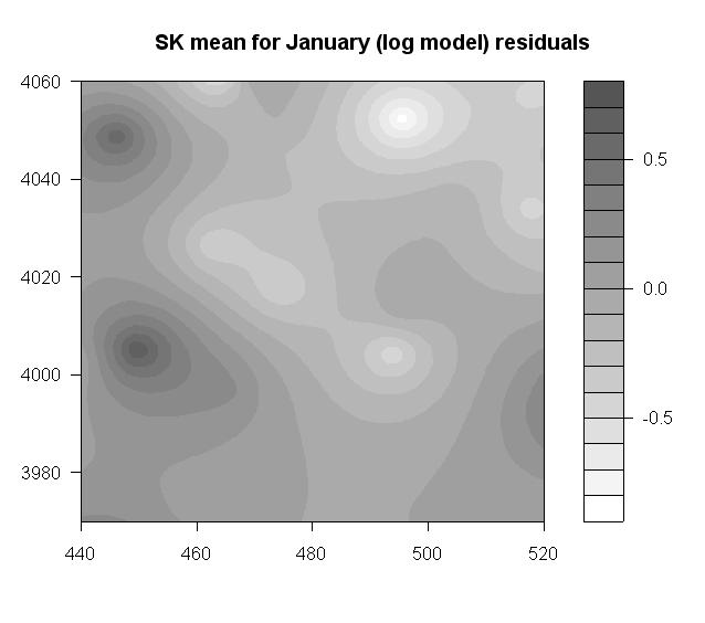
5 Example Northern NM precipitation, January log-model residuals The covariance function used in kriging is C(h) = e h/ , with the practical range of about 30. One look at the kriging st. dev. map tells us that we cannot reliably predict the precipitation (at least for January) in-between the stations. 5

6 Ordinary kriging (OK) The next issue will be estimating the mean m, which we assumed known in simple kriging. Option 1: first, estimate mean from the observations, then apply SK. Option 2: do both at the same time (Ordinary kriging). Option 1: We could try and estimate m by simply averaging the observations, but this does not take into account the correlations between V j. For example, if two locations are close together, and there is spatial continuity, then we have effectively one observation instead of two. This will require a Generalized least square approach, discussed later. Option 2: To keep the estimate unbiased, we need Thus, we need λ j = 1. m = E [V 0 ] = λ j E [V j ] = λ j m MSE is still expressed by (1), and we need to minimize it. We will apply Lagrange multiplier method of constrained optimization: minimize the function F (λ, µ) = MSE 2µ( λ j 1) where µ is the Lagrange multiplier. Taking partials with respect to λ k and µ and equating them to 0, we will get a system of equations { λ OK j C(k, j) µ = C(0, k), k = 1,..., n λ OK j = 1 In matrix form: C(1, 1)... C(1, n) 1 C(2, 1)... C(2, n) C(n, 1)... C(n, n) The kriging variance is, similarly to (4), λ 1 λ 2... λ n µ = σ 2 OK = C(0, 0) λ OK j C(0, j) + µ C(0, 1) C(0, 2)... C(0, n) 1 Overall, σ 2 OK is slightly higher than σ 2 SK because of higher uncertainty associated with estimating m. 6

7 Example continued Let s zoom in on a portion of NM precipitation map: the locations marked are stations close to the point x 0 = 470, y 0 = 4010, marked by. Comparing kriging st.dev. at that point, σ SK = , σ OK = , and maximum possible is σ = C(0, 0) = The kriging weights λ j were sorted according to their absolute values and the first 10 are: lambda_sk lambda_ok point no. [1,] [2,] [3,] [4,] [5,] [6,] [7,] [8,] [9,] [10,] Generally, closer points get higher weights. Notice, though, that 15 is masked by the presence of 14, and some stations get negative weights! 7

8 8