Optimal Interpolation

Transcription

1 Optimal Interpolation Optimal Interpolation and/or kriging consist in determining the BEST LINEAR ESTIMATE in the least square sense for locations xi where you have no measurements: Example 1: Collected SST ZI=? Estimated SST ZI = a Z1 + b Z2 + c Z3 Linear Estimate

2 Optimal Interpolation General Case: N measurements estimated data at location (xi,yi) linear coefficients: we attribute a weight to each collected data measured data at locations (xk,yk), k=1,...n How do we calculate the linear coefficients, wk? minimizing the estimated error variance! True Value error Estimated value

3 Optimal Interpolation ERROR VARIANCE where is the expected mean drawn form a large number of realizations or some large statistical population. NOTE: This large statistical population is usually not sampled, meaning a priori information must be given!

4 Optimal Interpolation We solve for the unknowns wk minimizing the error variance (similar to the least square problem) N unknowns, N linear equations! MATRIX FORM Do we still have a problem?

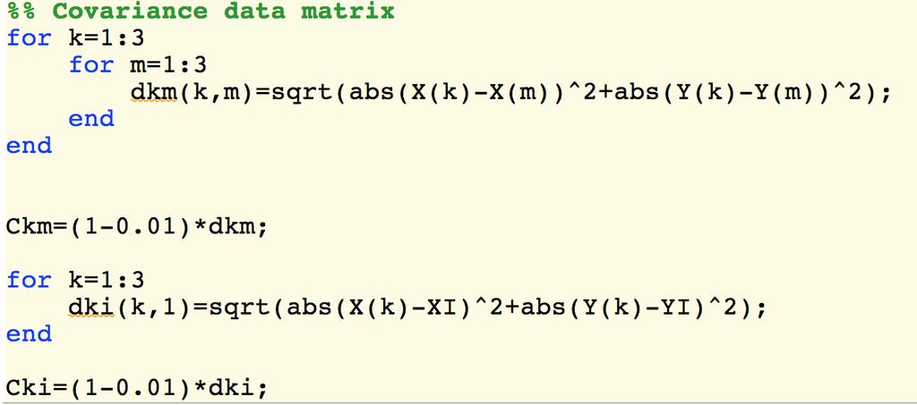
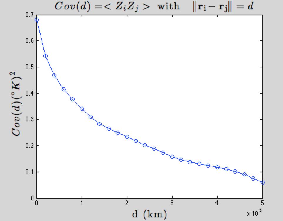
5 Optimal Interpolation Problems: The true values Zi is not known We have usually not sampled a large statistical population to estimate the <ZiZk>. We add a priori information to the problem: a covariance model, from which we are getting the Covariance Matrix The covariance between data collected at two locations depends on the distance that separates the two location NOTE: Z'k is the anomaly ( a spatial trend has been removed) refers to a spatial trend or mean

6 We go back to our linear system of N equations: We rewrite the problem using the anomalies (removing the mean or trend) We define:

7 In Matrix Form: estimated-data covariance vector data covariance matrix (a priori information) N x N if data at N locations linear coefficients ( weights ) for the optimal interpolation at location i

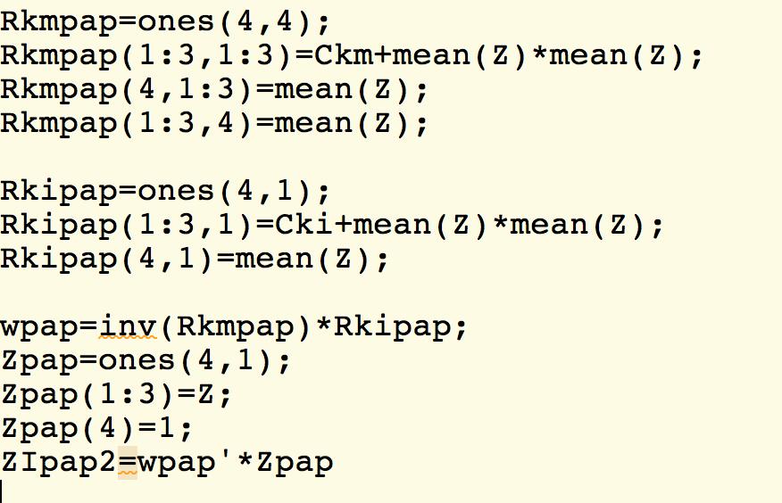
8 transpose NxN data covariance matrix Nx1 estimated-data covariance vector 1*N line vector of weights Nx1 vector of data estimated value at one location (xi,yi)

9 Computing the error in the mean square sense: Minimizing the mean square error has led to: Therefore:

10 Note: Therefore: 1) If no data available : Best estimate is the expected value Expected error is the Covariance of the data at zero lag

11 2) If data available : >0 The presence of data results in a reduction of the error by: Error variance estimate (or square error or confidence interval ) covariance of the data at zero lag expected error if no observations weights: nearby data that is expected to covary positively are assigned larger weights

12 Optimal Interpolation ordinary krigging We relax the assumption that we know the mean drift: To do so, we must add a constraint. In order to keep the estimate unbiased, this constraint must be: The problem now results in minimizing a function of N variables, the error variance that is function of the wk, with a constraint on the wk. Mathematically,we look for wk that satisfy:

13 In Matrix form:

14 Example:

15

16 Check that:

17 IF the MEAN is not removed: BAD ESTIMATE There is a better way of estimating the data, adding a variable ZN+1=1 (Papoulis, p393)

18

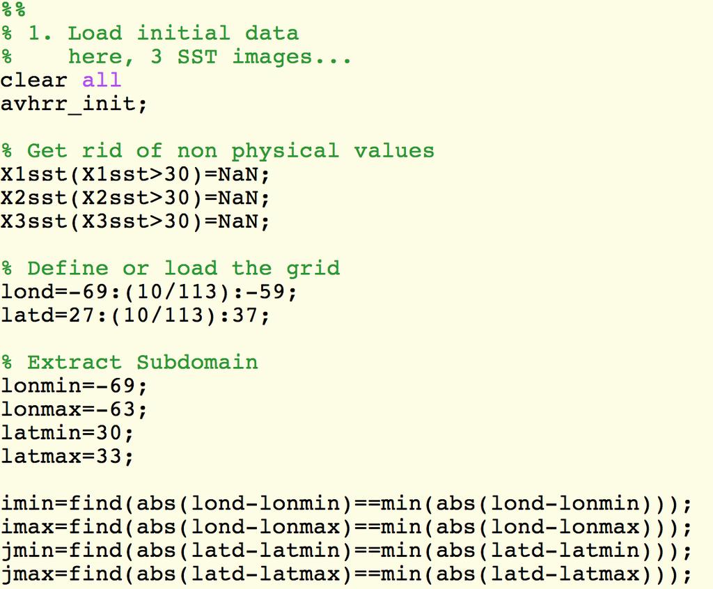
19 Example 2: AVHRR SST image with NAN values (due to clouds) 114 x 114 SST image with NaN values Objective: estimate the SST at locations where we have no data

20

21

22

23

24 The full image after filling the gaps with the ordinary krigging method

25 The error!!!!! The error is maximum at the points where we estimated data The error is maximum at points located far away (beyond d0) from good data, therefore it depends on d0 The amplitude of the error also depends on your variance (C0).

26 To do: Vary the parameter d0 chosen in the covariance model: choose large d0 and small d0 How can we objectively choose a covariance model and the parameters associated to it?

27 Variance and Covariance Variance of ONE variable Z: It is mean of square deviation of your data Covariance of TWO variables Zj and Zk:

28 Correlation Correlation coefficient of TWO variables Z j and Zk: It is a statistical measure of whether two variables are linearly related to each other perfectly positively correlated data uncorrelated data perfectly negatively correlated data Of course, if j=k, the two variables are identical, and they are perfectly correlated to each other

29 Auto Covariance Time Series You want to know to what extent the measurement you collected at time t+τ depends on the measurement you collected at time t Consider you have a times series of length N, with equally time spaced measurement Zk. We define the autocovariance because the two variables are the same) at lag nδt: Mean of the (N-n) data values starting from the n+1 measurement Mean of the (N-n) data values starting from the 1st measurement

30 Autocorrelation at zero lag: only difference with variance is the division by instead of (N-1)!

31 Z1 ZN-1 Z N Z2 C(0) Z1 ZN-1 Z N Z2 C(1) Z1 ZN-1 Z N Z2 Z1 Zn+1 Z2 C(n) Z1 Z2 Zn+1 2N+1 values with the zero lag at the middle: Czz(N)=cov0 ZN-1 ZN

32 Notes: Covariance has units! You may wish to compare several time series with different units. In that case, we use correlation. Correlation is a normalized form of covariance. Autocorrelation (when the two variables are the same): At zero lag, the autocorrelation is 1. In case of non periodic signal, it rapidly decreases as time increases. C(n) for n> N/5 usually not trustable

33 Example 1: Periodic signal... How does the covariance function look like? Title:./covariance-exemple1.eps Creator:MATLAB, The MathWorks, Inc. Vers CreationDate:03/17/ :20:30 LanguageLevel:2

34 Matlab solution: Analytic solution:

35 The covariance of a periodic signal is periodic! X axis is the lag n To convert it into unit: n Δt In our example, Δt=1 hour

36 Example 2: Mimicking a tidal signal... How does the covariance function look like?

37

38 Auto Covariance Spatial Data You want to know to what extent the data you collected at two locations separated by a distance d depend on each other. Consider data collected at N locations, equally spaced. We define the distance autocovariance ( because the two variables are the same) at lag nd: difficult to estimate C(d), computed from experimental data and plotted as a function of the distance lag d, is named the variogram

39 variograms (covariance) models commonly used for optimal interpolation Linear: Exponential: Gaussian: Spherical:

40 C0: Unresolved variance, or measurement error found as the intercept of the variogram at d=0. This is also named the nugget Cinfty: variance between uncorrelated data pairs as lag (d) goes to infinity; This is also named the sill d0: distance beyond which data points are no longer correlated. This is also named the range

41 Problem: Choose the SST image chosen as an example for the optimal interpolation Compute the lag autocovariance function, also named variogram of this image Fit one of the covariance model to your empirical variogram Apply it to your optimal interpolation.

42

43

44 TIPS: Check the physical aspect of your estimated data Is the estimated data in a respectable range of values? If not, what can I do? Modify the parameters of the covariance model... Check the covariance matrix (see on of the next point) Check the sensitivity of your method to the covariance model. Check the sensitivity of your method to the parameters of the covariance model (nugget, sill, range) Remember that the results of the method depends on the invertibility of the covariance matrix. This means that the matrix must not be singular. Why should it be singular at the first place? The data that you use to build the variogram may have some errors. Taking into account this error can help making the covariance matrix less singular Check the error given by the method.

45 NOTES: Measured data points will influence the estimated data within the range d0. Beyond d0, they will not estimate the solution of the interpolation. If you have no data, or estimated data located beyond d0, then the best estimate given by the method will be the mean, Z0. And the error will be maximal!

46 Adding some errors to the measurements We consider a sequence of two random variable, Zk (collected data) and Zsk(signal) related by the following relation: collected data true signal noise Our purpose is the same as before: it consists in estimating some data Zi using a linear combination of the the Zk, that minimizes the error in the least square sense function to minimize

47 Adding some errors to the measurements We consider a sequence of two random variable, Zk (collected data) and Zsk(signal) related by the following relation: collected data true signal noise Our purpose is the same as before: it consists in estimating some data Zi using a linear combination of the the Zk, that minimizes the error in the least square sense function to minimize

48 Adding some errors to the measurements

49 Adding some errors to the measurements Minimizing the error, looking for a local extremum: We can simplify the problem if we make the assumption that: 1) the noise attached to the measurement collected at location rm is not correlated to the noise attached to the data collected at location rk kronecker symbol noise variance 2) the signal is uncorrelated to the noise:

50 Adding some errors to the measurements

51 Adding some errors to the measurements

52 Adding some errors to the measurements

53 Adding some errors to the measurements Minimizing the mean square error has led to: Therefore: avec

54 SST ( C) Error (mean square sense) in ( C)2

55 To be done next year: Show that the error is orthogonal to the data, so that extremum that is found corresponds to a minimum Take an example from real data (fromvar, or TP rade)