Low-Level Monitoring of Bottlenose Dolphins, Tursiops truncatus, Charlotte Harbor, Florida Final Report. Contract 50-WCNF

Transcription

1 Low-Level Monitoring of Bottlenose Dolphins, Tursiops truncatus, in Charlotte Harbor, Florida Final Report Contract 50-WCNF Submitted to the U.s. Department of Commerce National Oceanic and Atmospheric Administration National Marine Fisheries Service Southeast Fisheries Center 75 Virginia Beach Drive Miami, Florida April 1996 R.S. Wells, M.K. Bassos, K.W. Urian, W.J. Carr, and M.D. Scott Chicago Zoological Society Sarasota Dolphin Research Program c/o Mote Marine Laboratory 1600 Thompson Parkway Sarasota, Florida 34236

2 Table of Contents Executive Summary Introduction Methods Study Area Survey Schedule Field Techniques and Logistics Photo-Identification Catalog Analysis of Photographs Data Processing Estimation Procedures Abundance Interannual Trends and Power Analyses Natality Mortality Immigration, Emigration, Residency, Transience Results Survey Effort Photo-ill Catalog Development Abundance Estimates and Trends Power Analysis Natality Mortality Immigration, Emigration, Residency, and Transience Discussion Photo-Identification Catalog Abundance Estimates and Trends Natality Mortality Immigration, Emigration, Residency, Transience Summary of Population Parameters Comparison of Abundance Estimation Methods Power Analyses Survey Design Recommendations Acknowledgments Literature Cited List of Tables List of Figures List of Appendices

3 Low-Level Monitoring of Bottlenose Dolphins, Tursiops truncatus, in Charlotte Harbor, florida, Final Report, NMFS Contract 50-WCNF Randall S. Wells, M. Kim Bassos, Kim W. Urian, William J. Carr, Michael D. Scott Chicago Zoological Society, Sarasota Dolphin Research Program c/ o Mote Marine Lab, 1600 Thompson Parkway, Sarasota, Florida Executive Summary The National Marine Fisheries Service (NMFS) has recognized a need for low-level monitoring of bottlenose dolphin stocks in southeastern U.s. waters, designed to detect catastrophic changes in the stocks. The main goals of the monitoring are detection of large-scale changes in dolphin abundance and establishment of archival databases for long-term trend detection. Low-level monitoring can provide a short-term means of detecting large-scale changes in population abundance and give decision makers the information necessary to determine if modification of management plans is necessary. To these ends, the NMFS has funded several local research efforts in the southeastern U.s., including the photographic identification effort in Charlotte Harbor, Florida, reported here. Charlotte Harbor was of interest to management agencies at least in part because of the use of this region from the 1960's through the 1980's for commercial dolphin collection. More recently, Charlotte Harbor has been designated as a National Estuary under the Clean Water Act. Our Charlotte Harbor study area included the inshore waters from Lemon Bay southward to northern Pine Island Sound on the central west coast of Florida. Photographic identification surveys were conducted through the study area on an average of 24 boat-days in August of each year from 1990 through Markresighting analyses modeled after a comparable study in Tampa Bay during allowed estimation of abundance and natality, analysis of inter-year trends, and evaluation of seasonal residency. Our Charlotte Harbor photo-id catalog for included 411 different dolphins. During August of each year from 1990 through 1994, an average of about 308 dolphins used the Charlotte Harbor study area. The abundance apparently increased from (95% CLs) in to in Part of this increase appeared to be due to an increase in reproduction. The average natality across the study years was 0.034, but a peak of was reached in The increase in the proportion of calves from in 1990 to in 1993 and 1994 suggests the successful recruitment of many of the young-of-the year. It was not possible to calculate rates of immigration or emigration. Evidence from the high proportion of animals present in multiple years and the absence of documentation of unidirectional movements between Charlotte Harbor and other adjacent and distant contiguous study areas along the central west coast of Florida indicate that permanent immigration and emigration appear to be rare events. About 9% of the

4 dolphins appeared to be transients. Immigration, emigration, and transience are not major influences on the number of animals present at any given time, but they ma y be important ecologically by providing a means of genetic exchange between populations, as demonstrated for the Sarasota dolphin community and for Tampa Bay. It was not possible to calculate a meaningful mortality rate, but stranding data mirrored patterns of mortality reported from other parts of the central west coast of Florida during the same period. We attempted to summarize the components of the interannual differences in abundance estimates. It appears that the increase in abundance from 1992 and 1993 may be attributed to a return to presumably normal mortality after high mortality the previous year, a higher-than-normal number of young-of-the-year recorded, a higher-than-normal number of calves recorded after a relatively low number recorded the previous year, and a higher-than-normal number of residents recorded in the area (due to increased movement into the area or more effective photographic effort). These data suggest that conditions in the area improved in 1993, particularly in comparison to 1992, with relatively high recruitment and possibly site fidelity, and improved survivorship. A number of recommendations were made as a result of the findings of this project. We recommend that monitoring be continued at least annually to track and evaluate the apparent trend. More-intensive surveys would permit more-refined determinations of natality, immigration, emigration, transience, and mortality. Although two or three annual surveys can detect large trends in abundance, this study illustrates the difficulty of interpreting the causes for the abundance changes without more detailed or longer-term information. Photo-ID work should be expanded to other seasons to examine previous reports of seasonal fluctuations in abundance. Empirical studies designed to identify the appropriate level of effort for mark-recapture surveys should be conducted. Photo-ID efforts should be expanded to greater distances offshore and along the coast to examine immigration, emigration, and transience in greater detail. Patterns of habitat use in Charlotte Harbor should be examined through integration of GIS habitat data with our sighting data. Efforts should be made to integrate ecological studies of the dolphins of Charlotte Harbor with other research efforts under the National Estuary Program. Dolphin community structure needs to be examined in more detail to define biologically meaningful management units. Existing information on residency, ranging and social patterns, and genetics should be integrated to arrive at population designations. Analysis of community structure is necessary to interpret immigration, emigration, and transience relative to population size. Sample sizes for examination of mt-dna haplotype distributions in Charlotte Harbor should be augmented through biopsy darting or capture-release efforts. The genetics data should be supplemented with telemetry data on movements and additional photo ID efforts. A correlation between increases in the number of dolphin strandings and the occurrence of red tide blooms suggests that further investigation into the role of red tide in dolphin mortality may be warranted. 11

5 Introduction The National Marine Fisheries Service (NMFS) is responsible for establishing quotas for take of bottlenose dolphins (Tursiops truncatus) and for monitoring the populations of dolphins in the southeastern United States waters. Quotas have been based on a rule-of-thumb developed by the Marine Mammal Commission in which the annual quota has been set at 2% of the estimated dolphin abundance for a geographical location. Most of the live-capture fishery for bottlenose dolphins has occurred in the coastal Gulf of Mexico and the Florida east-coast waters. In recent years, large scale mortalities of bottlenose dolphins have occurred in several locations in southeastern U.s. waters. The NMFS completed sampling surveys in these areas for abundance estimation, and recognized a need for low-level monitoring of bottlenose dolphin stocks in southeastern U.s. waters, designed to detect catastrophic changes in the stocks. The main goals of the monitoring were detection of large-scale changes in dolphin abundance and establishment of archival databases for long-term trend detection. Low-level monitoring could provide a short-term means of detecting large-scale changes in population abundance and give decision makers the information necessary to determine if modification of management plans is necessary. To these ends, in 1987 the NMFS began funding several local research efforts in the southeastern U.s. with the following stated objectives: 1) Detection of large-scale (halving or doubling) interannual changes in relative abundance and/or production of the bottlenose dolphin stocks in the southeast U.s. The population rate parameters of relevance include: a reliable index or estimate of local relative abundance, natality, mortality, emigration, and immigration. 2) Establishment of archival databases for long-term trend detection in localized geographical regions around the southeast US. One of the regions selected by the NMFS for low-level monitoring was Charlotte Harbor, along the southwestern coast of Florida. Charlotte Harbor was of interest to management agencies at least in part because of the use of this region for commercial dolphin collection. In addition to those removed by several active collectors prior to regulation under the Marine Mammal Protection Act of 1972 (R. Wells, pers. obs.), 43 dolphins were collected from these waters during (Scott 1990). More recently, Charlotte Harbor has been designated as a National Estuary under the Clean Water Act. Aerial surveys to estimate bottlenose dolphin abundance in Charlotte Harbor have been conducted on four occasions since 1975: by Odell and Reynolds (1980) during , and by the National Marine Fisheries Service during , , and 1994 (Thompson 1981; Scott et ai. 1989; Blaylock et ai. 1995). The aerial survey study area included Charlotte Harbor proper, as well as Pine Island Sound to

6 the south, and Gasparilla Sound to the north. The results of these surveys are summarized in Table 1. The approach selected for the low-level monitoring of Charlotte Harbor dolphins was photographic identification (photo-id) surveys from small boats (see reviews by Scott et al. 1990a; Wiirsig and Jefferson 1990). This technique has proven effective in long-term studies of population-rate parameters in contiguous waters of Sarasota Bay, immediately to the north (Wells and Scott 1990), and Tampa Bay (Wells et al. 1995), the next bay system to the north of Sarasota. The residency suggested by tagging studies in (Irvine and Wells 1972) and 1984, and longterm resightings of distinctive dolphins photographed by Wells (1986) during surveys initiated in 1982, indicated that Charlotte Harbor would be appropriate for photo-id surveys. Photo-ID offers several advantages over aerial surveys for measuring certain population rate parameters. The greatest advantage of using photo-id methods is the accumulation of information on the occurrence, distribution, and ranging patterns of specific individuals. The ability to recognize individuals over time provides opportunities to estimate abundance using mark-resight methods, to evaluate possible cases of immigration, emigration, or transience, to monitor individual female reproductive case histories, to determine the origins of carcasses for mortality estimates, and to examine community structure (Wells 1986). This report summarizes the results of five years of NMFS-sponsored bottlenose dolphin research in Charlotte Harbor, conducted by the Chicago Zoological Society (CZS). Annual photo-id surveys were conducted during August of each year from 1990 through The study area included more than half of the region of the aerial surveys, but did not include all of Pine Island Sound, due to logistical and budgetary constraints. Photographs and sighting data were collected to examine trends in abundance, natality, mortality, immigration, and emigration. Methods Study Area The Charlotte Harbor study area includes the enclosed bay waters eastward of the chain of barrier islands from the north end of Lemon Bay southward to Captiva Pass, as well as the shallow Gulf coastal waters and passes immediately surrounding the barrier islands (Figure 1). The southern boundary of the study area extends from Captiva Pass, through northern Pine Island Sound to Matlacha Bridge, east of Pine Island. To the northeast, the study area extended to the Rt. 41 bridge over the Peace River in Punta Gorda, and the EI Jobean bridge over the Myakka River. The region is composed of a variety of habitats and conditions, including highly productive seagrass meadows and mangrove shorelines, deep passes between barrier islands, shallow, sandy Gulf waters, dredged channels, river mouths, and open bays.

7 3 This study area was selected in part because of its proximity to the long-term Sarasota study site (Scott et al. 1990b; Wells 1991). Preliminary studies indicated that a number of distinctively marked dolphins inhabited the region, and at least some were present over a number of years (Irvine and Wells 1972; Wells 1986). The photo-id research being conducted in the Sarasota (ongoing) and Tampa Bay (through 1993) waters to the north facilitated examination of immigration and emigration. Inclusion of the Charlotte Harbor study area completed a nearly 200 km long section of contiguous coastline for which movement patterns of bottlenose dolphins could be determined. The Charlotte Harbor study area provided a unique opportunity for comparison with population rate parameter data collected from the Sarasota study area. Strong similarities among the areas allowed some measure of control for the effects of habitat on population parameters. The Charlotte Harbor study area is a mirror image of the Sarasota study area, in terms of geography. Physiographically, the areas are nearly identical, with bays of shallow seagrass meadows separated from the Gulf of Mexico by long, narrow barrier islands. The bays communicate with the Gulf through narrow passes. Each study area opens at one end into a large deepwater, estuarine embayment, and each is restricted at the opposite end to a narrow, artificially-maintained waterway. Both areas are of similar size. The Charlotte Harbor area is much more nearly pristine than the Sarasota area, however. We have divided the 701-km2 study area into five regions for assessment of survey effort (Figure 1). Regions were identified by physiographic and effort criteria. Because of the distances of some parts of the study area from our field stations, it was not possible to survey all of Charlotte Harbor with uniform effort. The segmentation was done in order to be able to quantify effort in different parts of the study area in an attempt to make the within-region effort comparable across years. The northernmost section, Region 1, includes Lemon Bay, a shallow bay with a narrow dredged Intracoastal Waterway (ICW) channel and Stump Pass, a variably navigable inlet from the Gulf of Mexico. Water depths range from less than 1 m nearshore to 6 m in the Pass, but generally waters were 2 m or less. Coastal development, primarily residential, was greater in this region than in all others. Region 2 included Gasparilla Sound, Placida Harbor, Gasparilla Pass, and Bull and Turtle Bays. Waters were generally less than 2 m deep, except for the dredged ICW channel and a basin in Gasparilla Sound, where depths ranged up to 3 m, and Gasparilla Pass, where depths reached 7 m. Bull and Turtle Bays are very shallow, undeveloped, mangrove-fringed bays with extensive coverage by seagrass meadows. Between these bays and Charlotte Harbor to the south is a wide band of shallow waters, less than 2 m deep. Coastal development in this region in general is intermediate between Region 1 and the remaining regions. The next section to the south, Region 3, includes a large inlet, Boca Grande Pass, and the open waters of Charlotte Harbor proper, along with the shallow southeastern coastal waters. Boca Grande Pass is the primary connection between Charlotte Harbor and the Gulf of Mexico, with depths of up to 24 m. Charlotte Harbor is about 3 m to 7 m deep

8 through its east-west axis, with fringing shallows of less than 2 m. Region 4 is the continuation of Charlotte Harbor to the north and east, to the mouths of the Peace and Myakka Rivers. The open waters of the north-south axis of Charlotte Harbor are generally 3 m to 7 m deep, with fringing shallows of less than 2 m depth. Freshwater inflow from the rivers varies seasonally, but continues year-round. Little development is evident except at the mouths of the rivers, especially the town of Punta Gorda on the Peace River. Region 5 includes the shallow waters to the south between Charlotte Harbor and Pine Island Sound. This region includes numerous sandy shoals and small mangrove islands, with channels through some of the shoals and seagrass meadows. Depths average less than 2 m in most areas, ranging up to 3 m to 4 m in the channels. Low levels of residential development occur on some of the islands. Survey Schedule A two- to three-week window during August was selected to provide ample opportunity to fully survey each region of the study area at least three to five times. This timing was selected for several reasons. Late summer historically brought a period of calm weather, providing a window of favorable survey conditions before the cold fronts begin to penetrate southward into central Florida. The timing was also considered to be advantageous for natality estimates. In adjacent waters to the north, most of the year's calves were born by late summer (Wells et ai. 1987; Urian et ai. in press). Based on an assumption of similar patterns of reproductive seasonality, it seemed that a late summer survey would provide the best estimate of numbers of calves born during that year (young-of-the-year). Additional information on the occurrence of identifiable dolphins in Charlotte Harbor was provided by occasional surveys during other times of the year. Data from outside of the NMFS survey period each year were not included in quantitative analyses for this report, but provided perspective. Field Techniques and Logistics Surveys were conducted from 6-7-m outboard-powered boats. Two or, during later years, three boats were used during each survey. Each boat was equipped with a VHF radio, depth sounder, compass, thermometer, and eventually a hand-held LORAN. Survey crews ranged in size from two to six people per boat. Survey routes were selected each day based on predicted weather conditions and the status of survey coverage. While searching for dolphin schools, the boats were operated at the slowest possible speed that would still allow the vessel to plane, typically 33 to 46 km/hr, depending on the vessel. Once schools were encountered, the boats were slowed to match the speed of the dolphins and moved parallel to the schools to obtain photographs. Every dolphin school encountered along a survey route was approached for photographs. We remained with each dolphin school until we were satisfied that we had photographed the dorsal fin of each member of the school, or until conditions precluded complete coverage of the group. A suite of data including

9 5 date, time, location, activities, headings, and environmental conditions were recorded for each sighting. Numbers of dolphins were recorded in real time as minimum, maximum, and best point estimates of numbers of total dolphins, calves (dolphins ~ about 80-85% adult size, typically swimming alongside an adult), and young-of-the-year (as a subset of the number of calves). A young-of-the-year is defined as a calf in the first calendar year of life and is recognized by one or more of the following features: (1) small size; 50%-75% of the presumed mother's length, (2) darker coloration than the presumed mother, (3) non-rigid dorsal fin, (4) characteristic head-out surfacing pattern, (5) presence of neonatal vertical stripes, (6) consistently surfacing in "calf position" alongside the dorsal fin of the mother. The specific parameters recorded are defined, and a sample data sheet is presented, in the Appendices 1 and 2. We used Nikon camera systems (FE, F3, 2020, 8008) with zoom-telephoto lenses, motor drives, and data backs to photograph each school. Over the course of the project, longer lenses (up to 300 mm) and auto-focus cameras and lenses were incorporated, resulting in improved photo quality, and decreasing the time required to obtain satisfactory photographic coverage of each group. Kodachrome 64 color slide film was used throughout the surveys. The fine grain of this film provided excellent clarity for resolution of fin features. Color film allowed evaluation of the age of some wounds and fin features. The survey team was based on Don Pedro Island, at the southern end of Lemon Bay, near the southern extent of Region 1. This field station was 42 km from the farthest edge of the study area in Region 4, 32 km from the most distant point in Region 5, and 23 km from the most distant point in Region 6. The long distance and the large areas of exposed waters in Charlotte Harbor meant that the boats often faced abrupt changes in weather conditions and sea states during any given day, at times preventing us from reaching or adequately covering some regions. To facilitate access to the more distant regions, we began using a third boat in 1993 to reduce the time required to cover these areas. Photo-Identification Catalo~ The patterns of nicks, notches, and scars on the dorsal fin and visible body scars have been used successfully in numerous studies of bottlenose dolphins to identify individuals over time (Scott et al. 1990a; Wlirsig and Jefferson 1990). Our photographic catalog is based on exclusive categories that classify individuals with similar features together. Each of the 12 categories of the catalog is based on: (1) the division of the trailing edge of the dorsal fin into thirds and distinctive features located in each third; (2) distinctive features on the leading edge of the fin; (3) distinctive features on the anterior portion of the peduncle and (4) evidence of permanent scarring or pigmentation patterns on the fin or body. The primary photo-id catalog is composed of the most diagnostic and best quality original slides of each animal, filed alphabetically by each individual dolphin's unique four-character code. Prints are made from the original slides and

10 6 filed in a working catalog used for initial searching for matches. A duplicate catalog made from color photocopies of the color prints is maintained off-site as a backup copy. We maintain three photo-id catalogs that represent our different study areas: the Sarasota Bay region, Charlotte Harbor, and Tampa Bay and the inshore waters of the Gulf of Mexico. The catalog used for these analyses is a subset of a larger catalog incorporating dolphins sighted outside of the limited Charlotte Harbor region considered for this report. All catalogs are ultimately searched before an addition is made to the appropriate catalog. The photo-id catalog for the surveys included 16 dolphins first identified from the Charlotte Harbor study area during 1982 through We collaborated with Dr. Susan Shane in examination of 272 identification photographs taken by her in Pine Island Sound during her behavioral studies (Shane 1987, 1990a,b). Examination of these photographs resulted in 24 matches with animals in our identification catalogs for all areas, including 12 matches with our Charlotte Harbor catalog. As of September 1995, there were 2,247 dolphins (1,870 distinctive non-calves) in the DBRI photo-id catalogs for all study areas, including Charlotte Harbor. Analysis of Photographs Photographic slides are labeled with information from the corresponding sighting: date, film roll number, sighting number, and location code. Labeled slides are filed chronologically in archival-quality storage pages in binders. Comments from sighting data sheets are read for clues and additional information to ass i ~t in identification of animals (for example, distinctive features noted in the field, or features distinguishing between two similar animals). Each slide is examined using a IS-power lupe eyepiece to find all distinctive dolphins. Slides are sorted by each identifiable individual within a sighting and the best-quality slides of each animal showing the distinctive features of the fin are selected to compare with the photo-id catalog. The most prominent feature of the fin is identified and the category that best describes that feature is searched for a potential match. Matches are often made by comparing the slide directly to the print in the catalog. However, with a close match or to distinguish between fins with similar features, the original slide is used for comparison. To verify a match between similar fins, both fins are projected using a slide projector with a zoom lens and traced to line up distinguishing features. To confirm long-term, long-distance, or difficult matches, three experienced photo-id researchers examine the potential matches and must vote unanimously on the final match. When a match is made with a fin in our catalog, all slides are labeled with the dolphin's unique 4-character code and its name, and the dolphin is scored as a positive identification. When a match is not found in the first category searched, all other possible categories are searched to account for dolphins that have multiple identifying characteristics. The entire catalog is searched before a new animal is added to the

11 7 catalog. If we are confident the fin is reliably recognizable, the dolphin is given a name that describes the most obvious feature of the fin and a unique 4-character code that abbreviates the name is selected. To be considered a catalog-quality image, a new entry into the catalog must meet the following criteria: the entire fin, from the anterior insertion to the posterior insertion of the dorsal fin and the trailing edge of the fin must be visible, the image must be in focus and perpendicular to the photographer, and, when available, both right and left side images of the fin are selected for the catalog. The best-quality slide is labeled with the name, code, and catalog category that describes the most prominent feature of the fin. A print is made and added to the print catalog and the original slide is filed alphabetically in the slide catalog. An animal was occasionally "visually confirmed" in the field when it was recognized because it was familiar to an observer and it was counted as a positive identification for photo-analysis even though it may not have been documented photographically. For photo-analysis, a calf or young-of-the-year is considered positively identifiable only if it can be recognized because of distinctive features that make it identifiable independent of its mother. A small animal that appears in all slides next to a larger animal in the "calf position," (i.e., alongside and slightly behind the presumed mother), is assumed to be a calf. If the calf is with an identifiable mother, but the calf is not distinctive, it is not scored as a positive identification. In some cases it is possible to identify animals in a sighting that are not sufficiently distinctive to make long-term matches, or appear distinctive but are unidentifiable because the entire fin is not visible, photo coverage is incomplete, or photo quality is substandard. Each of these dolphins is classified as an "other... " with some reference to the most distinguishing feature. Although it is not considered a positive identification, an "other... " dolphin is counted toward revision of the group-size estimates. Fins that lack distinctive markings are considered "clean" but may also be used in calculating or adjusting group size estimates. In some cases, "clean" fins may be distinguished from one another within a sighting based on differences in fin shape. This minimum count of "clean" fins is added to the positive identifications and "other" fins to calculate the minimum, maximum, and best group size estimates. Thus, the minimum estimate is a minimum count of distinguishable fins within a sighting. A grading system that integrates recognizability, photographic quality, and coverage is used to identify the quality of a given sighting: Grade-l - All dolphins in the group were photographed or otherwise positively identified. All the animals in the best field estimate are accounted for as a) confirmed positive identifications; or b) as individuals that can be

12 8 distinguished within a sighting from a high quality photograph but do not warrant status as a 'marked' dolphin in the catalog. Grade-2 - There are photographs of some dolphins with distinctive fins that may be in the catalog, but because of the quality of photographs it is not possible to make appropriate comparisons with the catalog and make a match or assign an identification. Grade-3 - Photographic coverage is known to be incomplete, because all dolphins were not approached for photographs, no photos were taken, film did not turn out, sighting conditions were poor, etc. Data Processing Sighting data and results from photo-analysis are entered into the Dolphin Biology Research Institute (DBRI) database. As of September 1995, the database includes 10,307 sighting records of dolphin groups from Sarasota Bay, Tampa Bay, Charlotte Harbor and the inshore Gulf waters from 1975 through We use the FoxBase+ /Mac Version 1.1 relational database management system containing dbase programming language that permits us to write specific programs to manipulate the database. A Macintosh IIsi computer is used for data entry and a Macintosh Centris 650 computer is used primarily for data manipulations. We defined our dataset based on temporal and geographic criteria. We included sightings collected during the August surveys of 1990, 1991, 1992, 1993, and 1994 within the designated boundaries considered to comprise Charlotte Harbor (Figure 1). Group size estimates were derived from adjustments of field estimates based on photo-analysis (see Appendix 2). Minimum, maximum, and best field estimates were increased if the sum of the number of positively identified individuals plus the number of "other... " dolphins, plus the number of "clean" dolphins exceeded the original field estimates. The resulting revised minimum, revised maximum, and final best estimates were used in all calculations involving group size. Several of the abundance and trend estimates and the power analyses were conducted at the Inter-American Tropical Tuna Commission with a VAX 3100/80 micro-computer and a 486 IBM-compatible personal computer. Linear regressions were performed using a SAS procedure (SAS 1989). A FORTRAN program designed for use on IBM-compatible personal computers (TRENDS2; Gerrodette 1993) allowed us to conduct a power analysis to detect trends in abundance (Gerrodette 1987). Estimation procedures: Abundance The basic questions considered by this project were: "How many dolphins use the Charlotte Harbor study area during the August survey period, and how does this number vary from year to year?". A closed population was assumed because of the brief period during which the surveys took place each year. There are a variety of ways to calculate indices of abundance of bottlenose dolphins inhabiting Charlotte

13 9 Harbor. We followed the analytical procedures of Wells et al. (1995) as applied to bottlenose dolphins in Tampa Ba y during a similar study. Method 1 (catalog-size method) simply involves tallying the number of positively identified ("marked") individuals (M) sighted within the study area during the survey period. We derived our overall catalog of marked animals for each survey year by considering all sightings during the survey period regardless of the photo grade. The inclusion of a fin in the catalog was dependent on the recognizability of a dolphin, not the overall quality of coverage of a sighting. The catalog-size method does not account for dolphins that are not distinctively marked. The size of the annual Charlotte Harbor catalog (M) is an integral part of each of the following three abundance estimation procedures. Assuming comparable levels of sighting effort from year to year, the catalogsize approach may provide a reasonable index for detection of trends of abundance. To conduct a power analysis, however, a coefficient of variation (CV = vari12 I N) could only be calculated by considering each year ( ) as a replicate sample. A regression analysis of the five annual estimates was conducted to remove the effects of a potential trend; a CV was then calculated from the residuals. Method 2 (mark-proportion method) calculated the proportion of positively identified dolphins (m) relative to the total group size (n) in each sighting of "Grade-I" quality. The accuracy of the population-size estimates depends on the confidence in identifications. Therefore, only Grade-I sightings were used to derive the proportion of marked animals. There was no relationship between group size and the proportion of dolphins identified (r2 = 0.002). The proportions of marked dolphins to group size (min) for each sighting were averaged for each year. The total number of marked dolphins in the catalog for a given year (M) was divided by the average proportion of marked dolphins to yield an annual population estimate (N). A similar method was used by Shane (1987) to estimate abundance in Pine Island Sound. A 2000-replicate non-parametric bootstrap resampled the min proportions from observed groups to produce variance estimates and percentile confidence limits. Method 3 (mark-resight method) uses the Bailey modification of the Petersen method to estimate abundance (Bailey 1951; Seber 1982; Hammond 1986). The Bailey modification incorporates resampling with replacement in the model. Because both marked and unmarked dolphins may be resighted multiple times, this modification was deemed appropriate. The equation used was: N = M (n2 + 1) I (m2 + 1) with a binomial variance of

14 10 where N is the population size, M is the total number of different marked dolphins sighted during the year, n2 is the total number of dolphins sighted during all complete surveys of the area, and m2 is the total number of marked dolphins sighted during the same surveys. A complete survey consisted of a combination of daily surveys that covered all of the regions (Figure 1) once during good or excellent sighting conditions. These combinations were developed a posteriori for the purpose of testing this estimation technique. Each "complete survey" required three to six boat days over periods of three to fifteen days for completion due to the large area to cover and the incidences of poor weather conditions. Only "Grade-I" sightings were used to ensure that all marked dolphins present during these sightings were identified and the group size was accurately counted. Because of the difficulties of covering such a large area, only 2-3 complete surveys were conducted each year. CVs were calculated from binomial variance estimates. Method 4 (resighting-rate method) attempts to first estimate the number of unmarked dolphins (u) in the area and then add them to the number of marked dolphins in the catalog sighted that year (M) to estimate N. By assuming that unmarked dolphins are resighted at the same rate as marked dolphins, the following equation would estimate the number of unmarked dolphins: where M is the number of different marked dolphins sighted during the annual survey period, n2 is the total number of dolphins counted from "Grade-I" sightings during the annual survey period, m2 is the total number of marked dolphins counted from "Grade-I" sightings during these same sightings, n2-m2 is the number of unmarked dolphins counted from these sightings, and M/m2 is the proportion of the number of marked individuals to the number of sightings of these marked individuals.. The population size is then estimated by N =M + u and a CV was estimated by the regression analysis described in Method 1. Estimation procedures: Interannual Trends and Power Analysis Linear regression analyses were conducted to determine whether a trend was present in the indices or estimates of abundance (i.e., the slope of the regression line of abundance vs. year was significantly different from zero). We used a power analysis to calculate the number of surveys or the CVs of the estimates required to detect a trend (Gerrodette 1987). The power analysis relates five parameters: alpha (the probability of making a Type-l error, i.e. conduding that

15 11 a trend exists when in fact it does not), the power, or 1 - beta (beta is the probability of making a Type-2 error, i.e. concluding that a trend does not exist when in fact it does), n (the number of surveys), r (the rate of change in population size), and the CV of the abundance estimate. Additionally, one must choose whether a t- or z distribution and a one- or two-tailed test is appropriate, and whether r changes exponentially or linearly. It is also necessary to determine whether the CV is constant with abundance, the square root of abundance, or to the inverse of the square root of abundance. Notice that the actual estimate is not used, only the coefficient of variation of the estimate. This estimate can be the actual abundance (population size as determined from mark-resight methods or censuses) or indices of abundance (such as total number of marked animals in the photo-id catalog for a particular year, or total number of dolphins sighted per surveyor time period). One of the objectives of this research was to determine whether the photo-id method could detect a doubling or halving of population size with 80% certainty. Thus, alpha = 0.05, beta = 0.20, power = 0.80, r = 1.00 or -0.50, n = 2 annual surveys, and it is only necessary to calculate the CV required to detect a trend and compare it with the CV of the abundance estimate calculated from the data. Alternatively, one can use the CV of the estimate to solve for n, the number of surveys necessary to detect the trend. In general, the lower the CV, the fewer the number of surveys required to detect a trend (Gerrodette 1987). For mark-resight estimates, the CV decreases as the proportion of marked animals in the population increases (Wells and Scott 1990). Traditionally in research, one is concerned mainly with alpha and Type-l errors. This is conservative when considering whether to accept an alternate hypothesis as truth or not, but may not be conservative from a management point of view. Such a case might occur when the null hypothesis that a population is stable is accepted when, in fact, it is declining (Type-2 error). Gerrodette (1987) applied power analysis to linear regressions of abundance. Because the question posed is whether a large change can be detected from one year to the next, and because we used an annual survey period as the sampling unit, the sample size (n), equals two. A linear regression is not feasible with only two data points, so it is necessary to compare two distributions presumed to have known variances rather than use a linear regression (TRENDS2 does this automatically). Given the initial parameters specified by the NMFS (alpha = 0.05, power = 0.80, r = 1.00 or -0.50, and n = 2), one can calculate the CV necessary to detect trends in abundance. We used a I-tailed t-distribution for the TRENDS2 program, and specified that rates of increase or decrease be exponential. We made this choice because an exponential function is more typical of biological processes and because detecting a 50% linear decline is a moot exercise given that the population would be reduced to zero at the end of the second year. TRENDS2 also requires that the model of the relationship between CV and abundance be specified. As suggested by Gerrodette (1987) and a graph of our data, the "CV proportional to the square root of abundance" option was selected. Given these parameters, a maximum CV of 0.05 is

16 12 required to detect an increasing trend and a CV of 0.07 is required for a decreasing trend. Assuming that the calculated estimates and variances are the true population parameters, then a less conservative z-distribution can be used and the maximum CVs would be 0.16 (increasing trend) and 0.23 (decreasing trend). Conversely, if a more-conservative 2-tailed test were used, the maximum CVs would be 0.02 (increasing trend) and 0.03 (decreasing trend). We chose the I-tailed t-distribution option because it better fits the situation of considering a change in only one direction at a time and because it could be argued that calculated variances may not truly represent those of the population. Estimation procedures: Natality Natality was calculated as the proportion of dolphins in each sighting considered to have been born within the calendar year. Though the total number of calves was recorded for each group sighted, only the subset of calves considered to be young-of-the-year was considered to be relevant to the measurement of natality (Wells and Scott 1990). The average proportion of young-of-the-year was calculated for each year. Estimation procedures: Mortality We obtained stranding records from the Southeast U.s. Marine Mammal Stranding Network (D. Odell, pers. comm.) for bottlenose dolphins recovered from southern Sarasota, Charlotte, and Lee counties from 1979 through 1994 to estimate a minimum mortality rate for the Charlotte Harbor area. We examined photographs of dorsal fins of carcasses provided by Bob Wasno of the Lee County Department of Community Services, Torn Pitchford of the Florida Department of Environmental Protection, and Mote Marine Laboratory's Marine Mammal Stranding Program. We used photographs of animals that died during the period 1990 through 1995 and were recovered within the counties encompassing the Charlotte Harbor study area. Stranding records from outside our specified study area may be included because the exact locations of strandings within Lee County were not available and Lee County waters extend beyond our Charlotte Harbor study area. Photographs of the stranded animals were examined to determine if the markings occurred post-mortem or if decomposition obscured recognition. Estimation procedures: Immigration / Emigration/Residency /Transience We were unable to calculate rates of immigration and emigration for the dolphins in Charlotte Harbor, because the criteria we have used in other areas (eg., Tampa Bay, Wells et ai. 1995) were too restrictive for use in this project. To calculate a rate of immigration, we needed to identify "permanent" movement into or out of the study area during our survey period. "Permanent" is defined as being present or absent for a period of at least two consecutive years (Wells and Scott 1990). For an immigrant, we would have to document that the animal was not present for at least two years prior to its first appearance in the catalog, and that it was seen in the study area during each subsequent survey session (for at least two years). Thus, by

17 [ 3 definition an immigrant would have to be absent during (to clearly establish its prior absence), first identified in 1992 (its year of immigration), and present during Similarly, an emigrant would have to demonstrate its presence by being seen since the beginning of the study and for at least two consecutive years before disappearing, and remaining absent for at least two years. Given these restrictions, the only year for which such analyses would be possible was This is the year for which we have the least data available, due to Hurricane Andrew bringing our field season to a premature close. In the absence of meaningful quantitative measures of immigration and emigration, we provide qualitative descriptions of residency and movements between study areas, and we present quantitative estimates of transience. Marked dolphins were considered to be "residents" during the survey season if they were identified in at least four of the five survey years. It must be recognized that this definition of residency is limited; the repeated occurrence of these animals during our surveys does not necessarily indicate a year-round presence. The incidence of transience was estimated by identifying individuals that were sighted in only one year of the five-year survey period and had no other sighting records in the DBRI database. The incidence of transience was calculated as the proportion of individuals that met the criteria above relative to the total catalog size for each survey year. This rate is probably an overestimate because it may include dolphins that in fact are not transients, but were missed during other surveys, died, or their fins changed without being detected. Results Survey Effort Surveys were conducted during windows of days each year (Table 2). The size of the window each year depended on weather and the number of boats available. Weather, induding Hurricane Andrew in 1992, adversely affected survey schedules. During the first years of the project, only two boats were used, but in 1993 and 1994 three boats were used. Survey effort was measured in two ways. One measure was a count of the number of boat-days. A boat-day was scored when a boat left the dock to search for dolphins. On average, 24 boat-days were spent in the study area each year (range = days, Table 2). A more refined measure of survey effort is the number of linear kilometers covered by our survey boats searching for dolphins within the study area. The total number of kilometers surveyed while "on-effort", (under excellent, good, or fair survey conditions, see appendix) are summarized in Table 2, and are presented by region to allow a comparison of within-region effort across years. Differences across years reflect the effects of weather, and the use of variable numbers of boats. Dolphins were seen throughout the study area, but they were not uniformly distributed. Larger groups tended to be found in the more open and deeper waters

18 [ ~ (Figures 2a-e). The total number of sightings and dolphins seen each year closely track the level of survey effort (Figure 3). On average, six or seven photographs per dolphin were taken each year. These results compare favorably with those of the Tampa Bay survey project (Wells, et ai, 1995). Photo-ID Catalog Deyelopment The level of survey effort was considered sufficient to warrant generation of abundance estimates based on mark-resighting analyses. This conclusion was supported by the high proportion of identifiable dolphins in the population (58% to 80%, Table 3), and the frequency distribution of resightings of identifiable dolphins within survey years (Figures 4a-e). About one quarter of the dolphins were sighted at least twice during a given survey year, up to a maximum of 8 times each. Our Charlotte Harbor catalog for included 411 different dolphins. The catalog size provides a minimum population estimate for the Charlotte Harbor study area ranging from 165 identifications in 1992 to 243 in On average, 55% of the dolphins in an annual catalog were also seen in either the previous or subsequent year, 51 % were seen two years earlier or later, 51% were seen three years earlier or later, 50% were seen four years earlier or later (Table 4). Photographs taken during the NMFS surveys built upon an existing Charlotte Harbor catalog initiated in 1982 (Figure 5; Wells 1986). Of the animals identified prior to the initiation of the surveys, 16 individuals were sighted subsequently during the surveys in As expected, during the initial years of the surveys many identified dolphins were added to the catalog. New fins were added to the catalog at a slower rate during subsequent years (Figure 5). The proportion of first-time identifications comprising the annual catalog each year declined from 99% in 1990 to 14% in These results are comparable to those from the Sarasota community (Wells and Scott 1990) and Tampa Bay (Wells et al. 1995), suggesting a relatively closed population for the Charlotte Harbor study area. Identifications added to the catalog over the years may represent changes to the fins of known animals, non-distinctive calves acquiring new markings (only a small number of calves are in our catalog), or animals that may have been missed in previous years. We found that overall there were few changes to fin markings throughout the surveys, and minor changes could be detected by a skilled observer familiar with the catalog. However, dramatic changes to fin markings could easily be undetected and could result in a previously identified animal being entered twice in the catalog. The stability of fin markings over time enhances the probability of resighting individuals. The high frequency of resighting individuals and the long-term sighting histories suggested a high degree of residency for some animals in the Charlotte Harbor study area during the survey period (Figure 6). The consistency of the catalog and stability of fin markings over time contribute to our confidence in

19 15 meeting the assumptions associated with generating abundance estimates from mark-resighting analyses. Abundance Estimates and Trends The catalog-size index (Method 1) resulted in minimum population estimates of 165 to 243 dolphins over the five years of the study, with an average of 203 (Table 3). The Method-1 estimates are known to be underestimates because they do not take into account the unmarked dolphins. Methods 2, 3, and 4 attempted to correct for this underestimation. Method 2 (mark-proportion method) calculated population-size estimates from proportions of marked animals relative to revised minimum, revised maximum, and final best group size estimates. The differences between minimum and maximum population-size estimates were so small that we present only the estimates based on the final best group size. The number of dolphins estimated by Method 2 ranged from 226 to 422, with an average of 302 (Table 3). Method 3 (mark-resight method) provided annual point estimates from the combined sightings made during two or three "complete surveys". The estimates ranged from 238 to 385 across all years, with an average of 313 (Table 3). Method 4 (resighting-rate method) provided annual point estimates ranging from 194 to 385 dolphins, with an average of 267 (Table 3). The abundance estimates were examined for trends across the five years of the surveys. Population-size estimates varied from one year to the next (Figure 7). The trends in abundance roughly followed variation in field effort, but the relationship did not appear to be strong. Comparison of 95% CL for Methods 2 and 3 (Figure 8) indicate a significant difference in the abundance estimates from the first three years compared to the last two years of the survey. Power Analysis The catalog-size index (Method 1) used a regression analysis of the five annual estimates to remove the effect of a potential trend and calculated a CV of 0.15 from the residuals (although no trend was apparent, a test with only five data points would be sensitive to outliers and would have low power). Given that alpha = 0.05, power = 0.80, r = 1.00 or -0.50, and CV = 0.15, we can then calculate the minimum number of surveys necessary to detect a trend. Three survey sessions would be required to detect a decreasing trend and four for an increasing trend. A bootstrap variance procedure applied to Method 2 (mark-proportion method) yielded CVs ranging from 0.04 to 0.06, with an average CV of This would allow an increasing or a decreasing trend to be detected in two surveys.

20 16 The CVs for the estimates for the mark-resight method (Method 3) ranged from 0.06 to 0.10, with an average CV of 0.08 for This would allow an increasing or a decreasing trend to be detected in three surveys. Method 4 (resighting-rate method) used the regression analysis described in Method 1 to yield a CV of Three survey sessions would be required to detect a decreasing trend and four for an increasing trend. Natality The natality rate, the proportion of dolphins considered young-of-the-year, varied during the course of the surveys, ranging from to (Table 5). If these rates are applied to the population size estimates derived by Method 2 (markproportion method), then annual estimates of 7 to 17 young-of-the-year are derived for the Charlotte Harbor study area. The mark-proportion estimates are used here because the variances were low, and the estimates for population size and natality were calculated in a similar manner, i.e. on a proportion-of-school basis. Mortality There were 116 records of stranded animals from South Sarasota, Charlotte, and Lee counties from ; 70 of these records were from 1990 to 1994 (Table 6, Figure 9). We were unable to calculate a mortality rate due to the bias associated with an increase in stranding response effort since the mid-1980s. Coastal development and boating activity on Charlotte Harbor waters have also increased dramatically, possibly contributing to the discovery of carcasses in previously isolated areas. However, there are still many remote and inaccessible areas within Charlotte Harbor where carcasses are unlikely to be found. All these factors confound determination of the actual number of strandings and make it impractical to calculate a mortality rate based on stranding records alone. In an attempt to distinguish between mortalities and other kinds of losses from the population, photographs of stranded dolphins were examined. A total of 30 photographs were available to compare with the photo-id catalog. Dorsal fins in photographs of 7 animals were deemed non-distinctive, i.e., they belonged to neonates, calves or otherwise had no diagnostic markings. Twenty;.three animals were considered distinctive and were used to compare with the photo-id catalog (Table 6). We identified 2 of the stranded animals: One animal was sighted in the first four years of the Charlotte Harbor surveys and stranded in March of The other was first identified in 1990 and died in November of Of the 411 dolphins in the Charlotte Harbor catalog, 165 were not seen during the last year of the study. Two of these (0.012) were confirmed as mortalities based on fin identifications. Immigration, Emigration, Residency, and Transience We were unable to develop a reasonable quantitative estimate of rates of immigration or emigration for Charlotte Harbor due to the brevity of the study

21 17 period, as discussed under "Methods". All available data indicate that permanent immigration and emigration were rare occurrences. None of the more than 900 dolphins identified from Sarasota Bay ( ) and Tampa Bay ( ), the adjacent waters to the north, nor the 272 dolphins in photographs provided by Shane from her Pine Island Sound study area immediately to the south, were identified as immigrants to the Charlotte Harbor area during our study. Conversely, none of the 411 dolphins identified from Charlotte Harbor waters during were observed to take up residence in Sarasota Bay or Tampa Bay. Residency to portions of the Charlotte Harbor study area was suggested by repeated sightings of some individuals in the same waters over multiple years. Sixteen of the 411 dolphins in the catalog (3.8%) were also seen in the area prior to the initiation of the surveys in Twelve of these were first identified during Twenty-seven dolphins (6.6%) were identified from the Charlotte Harbor study area during all five of the survey years; 97 (23.6%) were seen during at least four of the five survey years. We did not find animals with regular movements through the entire study area when we examined those seen in multiple years, and those with the requisite 15 or more sightings needed for description of a horne range (Wells 1978). Instead, we found clusters of sightings within localized areas, as has been described elsewhere along the central west coast of Florida (Wells 1986; Wells et al. 1995). For example, "CURL" was seen frequently in Lemon Bay during (Figure 10 a). Sightings of dolphins such as "THUV" ( , Figure 10 b), "HISC" ( , Figure 10 c), and "TSMD" ( , Figure 10 d) were concentrated in Gasparilla Sound. Long-term sightings of dolphin "RPPR" ( , Figure 10 e) were spread through both Lemon Bay and Gasparilla Sound. Sightings of dolphin "LGSL" ( , Figure 10 f) were concentrated in and near the deep waters of Boca Grande Pass. "TFLN" ( , Figure 10 g) was seen repeatedly in the shallows in northern Pine Island Sound. Dolphins "CLTO" ( , Figure 10 h) and "ZIGY" ( , Figure 10 i) were seen primarily in the open, deeper waters of southern and western Charlotte Harbor proper. Dolphin "POTP" ( , Figure 10 j) was seen primarily in the shallow waters of eastern Charlotte Harbor. Little can be said about the year-round residency of these animals, except that all of the catalog members identified prior to the surveys were seen in months other than August. While these examples provide documentation of the tentative existence of long-term home ranges in the Charlotte Harbor area, they should not be interpreted as indicating that all of the dolphins in the area fall into these patterns. Additional sightings during different seasons would be required to accurately assign horne ranges or other movement patterns to the dolphins in Charlotte Harbor. Movements back and forth between Charlotte Harbor and waters to the north were recorded for ten (2.4%) dolphins of the 411 in the Charlotte Harbor catalog. A few individuals, such as "DIPT" (Figures 10 k,l) appear to spend equivalent amounts of time in southern Sarasota, Lemon Bay, and Gasparilla Sound, suggesting the existence of a horne range connecting these two regions. Others, such as"ry34 "

22 18 (Figures 10 m,n) and "BSLC" (Figures 10 o,p), emphasize one region, Sarasota or Charlotte Harbor, over the other, but on occasion move between regions. The most extreme movements were made by "SLIT" (Figures 10 q,r). This dolphin was observed in eastern Charlotte Harbor in August 1990, and in southern Tampa Bay in July 1991, a minimum swimming distance of about 125 km. It was not possible to describe a pattern for this animal based on only two sightings. The longer-distance movements were similar to those demonstrated by Sarasota males making occasional excursions into Tampa Bay (Wells 1993; Wells et ai. 1995). The gender is known for only three of the ten dolphins moving between regions. Two of the dolphins traveling the longest distance between regions are known males ("BSLC" and "RY34"), whereas one of the dolphins for which sightings are more evenly spread across a more limited extent of border waters is a female ("BRDO"). None of the other seven dolphins have been seen with a calf of their own, suggesting, but not conclusively demonstrating, that they may be males. Limited movements between our Charlotte Harbor study area and waters to the south were indicated by matches with 12 of 272 photographs provided by Shane from her study area including southern Pine Island Sound and associated waters. These findings also supported the concept of local residency for dolphins in this region, since none of the dolphins matched between our Charlotte Harbor catalog and Shane's photographs were seen north of regions three and four of our study area. In addition, while another 12 Shane dolphins were identified in our records from nearby waters outside of our Charlotte Harbor study area, none of Shane's 272 dolphins were known from our Sarasota or Tampa Bay identification catalogs. Shane (1987) reported that several of her dolphins apparently inhabited horne ranges in Pine Island Sound. Thus, at least some of the Charlotte Harbor and Pine Island Sound dolphins appear to follow the horne range mosaic pattern seen elsewhere along the central west coast of Florida, in Sarasota and Tampa Bay (Wells 1986; Wells et ai ). Dolphins identified during only one year of the surveys were defined as transients. There were a minimum of six and a maximum of 34 dolphins per year that met our criteria for transience (Table 4) representing 4% to 14 9 /0 of the annual catalog size. This should be considered a maximum estimate, since it may also include animals present during multiple years but not identified because of undetected changes to the dorsal fin, or because they were not photographed. None of the "transient" animals was seen in the Charlotte Harbor study area outside of the survey season, nor were they seen in adjacent study areas, so their origins and destinations remain undetermined.

23 19 Discussion Photo-Identification Catalog The ability to identify individuals over time using natural markings has proved to be a valuable and benign research tool and a standard in population studies of marine mammals. Maintaining a photographic database of individual dolphins enables researchers to monitor not only population parameters but habitat use, social association and distribution patterns. The high proportion of marked dolphins and the high frequency of resightings underscores the importance of including only excellent quality images of distinctively marked individuals in the photo-id catalog. This minimizes subjectivity in the matching process and reduces the chance of making incorrect identifications or missing them altogether. The development and use of our photo-identification catalog has been tested in three study areas, including Charlotte Harbor, and has proven effective in each case. However, as the catalogs grow and we expand into different study areas, we recognize the utility of developing computer-assisted matching and archiving abilities. Abundance Estimates and Trends Comparison of the point abundance estimates from Methods 2, 3, and 4 indicates reasonable consistency across methods, and an indication of change from the first three years to the last two years of the study (Figure 7). In all cases the lower 95% CLs were greater than or equal to the minimum count provided by the catalogsize method. Thus, if we consider the most extreme 95% CL values to be the limits to our estimates, the number of dolphins using the Charlotte Harbor study area during the surveys was between 198 and 369 during , and between 315 and 463 during We attempted to identify the reasons for the apparent increase in abundance of dolphins in Charlotte Harbor during the later years of the survey. Contraindicative results for Methods 2 and 3 in 1990 confound evaluation of the significance of differences between 1990 and later years (Figure 8). An apparent increase from 1992 to 1993 and 1994 was also evident, but field effort limitations brought about by Hurricane Andrew complicate interpretation of this year's estimate. Consistent patterns were obtained for both Methods 2 and 3 for comparisons between 1991, and 1993 and 1994, however. Based on Method 2, the abundance estimate from 1991 increased 31% and 61 % in 1993 and 1994, respectively. For Method 3, the comparable increases were 40% and 45%. For perspective, this increase, within the summer season across years, is much smaller than the summer to winter increases of 176% and 223% reported by Thompson (1981) and Scott et al. (1989) for Charlotte Harbor and Pine Island Sound.

24 20 Though the increase does not represent an interannual doubling of the population, the change was significant, based on comparisons of 95% confidence limits (Figure 8). The increase was evident through all four abundance estimation methods, and it ran counter to the patterns of consistency across years demonstrated for Tampa Bay and Sarasota (Wells et al. 1995; Wells and Scott 1990). Our evaluation approach was to first examine corroborative indicators of the change, and then to test hypotheses about the possible biological or methodological source(s) of the increase. The apparent increase in numbers of dolphins during was corroborated by changes in the number of dolphins sighted per unit of sighting effort. For this analysis, we divided the sum of the final best point estimates of numbers of dolphins for each sighting for each year by the number of kilometers of survey transects for that year. This density indicator should be less prone to potential biases that might have resulted from violations of mark-recapture assumptions. The number of dolphins per km increased by 14% from 1991 through 1993 and 1994 (Table 7). This measure provided additional supportive evidence of an increase in the numbers of dolphins in Charlotte Harbor. We hypothesized three potential biological sources of dolphins to account for the increase: (1) through recruitment of young, (2) through an influx of new dolphins, andl or (3) from the return of previously identified individuals. If the increase was due to recruitment of young, then several expectations follow. If we assume that Charlotte Harbor is a relatively closed population unit, and the entire increase resulted from reproduction, then the number of young-ofthe-year during a given year should be greater than or equal to the change in abundance from the previous year. As can be seen from Table 5, production of young was nearly 2.5 times greater in 1993 than in At no time, however, does reproduction during one year entirely account for abundance increases in the next year. If recruitment of young accounted for some, but not necessarily all, of the apparent abundance increase, then the proportion of marked animals (min for Method 2, Table 3) should decline over the years, since identifying marks tend to be acquired with age, and calves tend to be less marked than older animals. The accumulation of young-of-the-year from several years of increased reproductive output should be reflected in increased numbers of unmarked calves and juveniles in later years. The proportion m i n did in fact decline, from 0.80 in 1990, to 0.58 in 1994, suggesting a dilution of the pool of marked animals by young, as-yet unmarked individuals. Any increase indicated from mark-recapture analyses that is due to recruitment of young, should be expected to be reflected by other indicators that are not based on marked animals. Increases in numbers of young-of-the-year should result in subsequent increases in calves. The number of young-of-the-year per kilometer of survey transect tripled from 1990 through 1991, 1992, and 1993 (Table 7).

25 2 1 The number of calves of all ages observed per kilometer of survey transect increased from 1990 values by 20% in 1991 and 1992, 40% in 1993, and 30% in 1994 (Table 7). Thus, it seems reasonable to conclude that at least a portion of the apparent increase in abundance of dolphins in Charlotte Harbor is the result of increases in reproduction during the course of our project. If reproduction accounts for only a portion of the increase in abundance, then the balance must come from an influx of non-calves, either new to the area, or residents that had not been identified in the middle years of the study. As described above, non-calves would be expected to have acquired markings over time. Thus, an influx of new animals should be reflected in an increase in the annual catalog size in later years. Such an increase was apparent, but not dramatic (Figure 5). The number of new animals added to the catalog each year declined from through , however, indicating that many, but not all, of the non-calves identified in later years were re-identifications of animals originally added to the catalog in earlier years. In addition, the average proportion of dolphins in the catalog in a given year that were identified in previous or subsequent years increased in (Table 4). This increase may be explained partially by fluctuations in the timing of seasonal increases in abundance. Aerial surveys by Thompson (1981) and Scott et al. (1989) have shown summer-to-winter increases of % in Charlotte Harbor and Pine Island Sound. If the main reason for the increased abundance was an influx of non-calves, then we would expect the proportion min to remain relatively constant over the five years. The fact that the proportion declined over the years suggests that more of the increase is due to reproduction than to an influx of older, bettermarked animals (Table 3). The source of additional non-calves in Charlotte Harbor was not the contiguous coastal waters to the north, based on the results of censuses in Sarasota and Tampa Bays. It seems likely that any additional dolphins would have originated in the Gulf of Mexico or Pine Island Sound. Thus we are left with a series of potential explanations for the apparent increase, none of which alone seems sufficient to explain the entire increase. In terms of relative contributions to the increase, it seems that recruitment of young had a greater potential effect than did reidentifications of earlier catalog members, and each of these accounted for more of the increase than did an influx of new noncalves. We examined the possibility that the increase was at least in part a result of methodological complications, perhaps exaggerating a smaller real increase in numbers of dolphins. The low CVs, only slightly larger than those obtained by Wells et al. (1995) for our first application of these estimation techniques, during the Tampa Bay surveys, argued against methodological problems. We explored them, however, because of several differences in methods between the two studies.

26 22 The primary methodological differences involved level of effort. We had fewer boat-days each year for the Charlotte Harbor surveys than for the Tampa Bay surveys due to budgetary limitations. Though the Charlotte Harbor study area was 82% as large as the Tampa Bay study area, we had only 56% as many within-studyarea boat-days each year compared to Tampa Bay. Fewer boat-days translated into fewer kilometers of survey transects, which meant less intensive photographic coverage of dolphins in the study area than was accomplished in Tampa Bay. This in turn might have affected the development of the identification catalog, resulting in an artificially low M in some cases. Differences in weather conditions from year to year resulted in varying geographical coverage within the study area, which may also have affected the size of M, and may have influenced min as well. Each of these factors is critical to the calculation of abundance estimates. Each of the abundance estimation procedures assumed that M accurately represented the pool of marked dolphins in the study area during the survey period, and was independent of level of effort. The high proportion of marked dolphins (m i n), the relatively consistent values for M from year to year, and the numbers of resightings of marked individuals over the course of each survey suggested that we had obtained reasonable coverage and established a representative identification catalog in Tampa Bay (Wells et al. 1995). In Charlotte Harbor, however, min declined over time, the numbers of resightings per individual were smaller than Tampa Bay (Figure 6), and M fluctuated across years. One way in which effort might influence M would be through uneven geographical distribution of surveys resulting in differential exposure to marked individuals. Given the existence of individual ranging patterns as proposed earlier in this report, decreased survey coverage of portions of the study area might mean fewer opportunities to photograph residents of those regions, resulting in a smaller and inaccurate M. Effort was not uniform across regions from year to year (Table 2). Adverse weather conditions made it difficult to reach the more distant regions, including Region 4 (Charlotte Harbor North) and Region 5 (northern Pine Island Sound, Figure I), during some years. Our survey coverage of these two regions in 1994 was approximately double the coverage during the early years, and M was greater than in any previous year. Region 5 was a potential source of complications regarding M both because coverage was variable from year to year, and also because it opened into greater Pine Island Sound to the south, a potential source of new dolphins or destination for previously identified dolphins, outside of our study area. We attempted to control for these complications by recalculating abundance estimates without including Region 5 sightings, or the marked dolphins sighted only in Region 5. This analysis showed that Region 5 had little effect on M or on the abundance trend. We considered the possibility that uneven geographical coverage could result in a biased min. If this ratio varies from region to region, then differential coverage could result in a biased overall ratio, as applied in Method 2. We found that the

27 23 ratio mi n was smaller in Regions 4 and 5 than in the other regions, and these regions were over-represented in the survey efforts of later years as compared to the other regions. This provided one potential explanation for the decline in the overall m i n in later years, and may have contributed to the apparent increase in abundance as evident from the results of Method 2. The "complete survey days" of Method 3 control for survey effort, however, and the general level of agreement between the results of Methods 2 and 3 suggest that a potentially biased m i n was not a major contributor to the increase in abundance. The level of effort in Tampa Bay was greater and more consistent from year to year than in Charlotte Harbor. For example, due to Hurricane Andrew coverage of all regions in 1992 decreased to 51 % - 65% of the kilometers surveyed in other years, with a concomitant decline in M to 68% to 93% of the levels from the other years. We examined the data for a direct relationship between survey effort and catalog size, by regressing M against number of boat-days and numbers of kilometers surveyed. No strong linear relationships were found, but M vs. boat-days approached statistical significance (r2 = 0.74, P = 0.06), hinting at the role of effort in the development of an adequate catalog. Our findings suggest that an optimal level of effort exists between that expended in Tampa Bay and that in Charlotte Harbor. Empirical studies designed to identify the appropriate level of effort for markrecapture surveys would be helpful. Thus, methodological problems did not appear to be, the primary factor in the increase in the abundance of dolphins in Charlotte Harbor. Though the reasons for the increase can not be fully explained with the information available, the increase appears to be real, and appeared to be contributed to by several factors. The low CVs associated with the abundance estimates provide additional confidence in the trends that are evident. It is recommended that future surveys attempt to eliminate some of the variables considered in the discussion above by striving for more intensive, uniform effort throughout the study area. It is difficult to interpret comparisons of our abundance estimates to those reported from aerial surveys of Charlotte Harbor, because of methodological differences, and because of differences in the areas surveyed. The 'aerial surveys typically reported abundance estimates from Charlotte Harbor and Pine Island Sound combined, whereas our vessel surveys only included the northernmost portion of Pine Island Sound, due to logistical constraints. Our average abundance estimate from Method 2 (mark-proportion) for our limited survey area was comparable to the upper 95% CLs reported from the same season by Thompson (1981) and Scott et al. (1989) for their larger study area. As has been noted in other comparisons of vessel vs. aerial surveys (Scott et al. 1989; Wells et al. 1995), the aerial surveys appeared to have underestimated the numbers of dolphins in Charlotte Harbor. The estimates we have derived reflect the numbers of dolphins found in the Charlotte Harbor study area at least once during a two- to three--week period in

28 August of each year. The estimates are based on a catalog that includes all of those dolphins for which satisfactory identification photographs were obtained during the survey period, without distinguishing betvveen differences in the degree of use of the study area waters by different dolphins. The catalog makes no distinction betvveen those dolphins using the waters of the study area on a regular basis vs. those photographed during an infrequent passage through the study area. A number of overlapping home ranges occur along the central west coast of Florida, including Tampa Bay, Sarasota Bay, and Charlotte Harbor (Wells 1986), and home ranges apparently exist in Pine Island Sound (Shane 1987). The degree of overlap in home ranges in the Charlotte Harbor study area appears to vary. The probability of finding a given dolphin occupying a partially overlapping home range would be a function of the degree of overlap. The limits of our study area were not biologically based. They did not necessarily coincide with home range boundaries, for example, and therefore do not address the relative importance of waters and habitat features in the study area. Evaluation of the biological basis of population units has important management implications, but this requires more-detailed analysis of the community structure of dolphins in the Charlotte Harbor area. Natality Natality is likely underestimated because, if a diffuse calving season is assumed, then it is likely that some young calves were lost prior to each annual survey, and some may have been born after the survey. A spring through early fall peak in calving with occasional births occurring at anytime during the year has been reported for Sarasota Bay (Wells et al. 1987) and for the west coast of Florida in general (Urian et al.. in press). Thus, the actual crude birth rate may have been higher than the to reported from the surveys. The average Charlotte Harbor natality estimate of for the period is comparable to that reported for Tampa Bay for ( , Wells et al. 1995), and slightly lower than that reported for Sarasota Bay ( for Sarasota dolphins was calculated for the period (Wells and Scott 1990). Observational effort in Sarasota has been ongoing, providing opportunities to observe a higher proportion of births. The narrow window for the Charlotte Harbor survey means that some calves are more likely to be missed. Thus, the Charlotte Harbor natality measure should be compared to a Sarasota measure betvveen the crude birth rate and the recruitment rate (the proportion of calves surviving to age 1). For Sarasota Bay, the mean recruitment rate for was ± (Wells and Scott 1990). Therefore, a comparable measure of Sarasota natality might be betvveen and The variation in the natality rate over the five-year survey period also supports the conclusions drawn from the abundance estimates regarding the increase in population size.

29 25 Mortality Measurements of dolphin mortality rates for Charlotte Harbor proved to be difficult to obtain during our survey period. In most cases we were unable to distinguish between mortalities, emigrations, undetected fin changes, and animals missed during the Charlotte Harbor surveys. In Sarasota, it has been possible to evaluate losses from the population from two directions, through the collection and examination of carcasses of identifiable individuals, and through records of disappearances of known individuals (Wells and Scott 1990). Mortality estimates are facilitated in Sarasota as compared to the Charlotte Harbor project because Sarasota involves a smaller number of dolphins with a higher proportion of them being identifiable, a smaller study area, a more-intensive, year-round monitoring effort, and more-complete and consistent stranding response effort. The number of strandings reported during the Charlotte Harbor survey may, however, provide a relative index for comparison of mortality patterns. Dolphin strandings in Sarasota Bay, Tampa Bay and more generally along the central west coast of Florida followed the Charlotte Harbor pattern of dramatic increase from 1990 to , with a decline in 1993 (Wells et ai. 1995). In Sarasota, strandings reached levels two to three times normal from late 1991 through 1992 resulting in a 10% decrease in the size of the Sarasota population (unpublished data). No such decline was observed in Charlotte Harbor, however. Severe red tides from blooms of the dinoflagellate Gymnodinium breve occurred along the central west coast of Florida during 1991, 1992, and 1994, the years of greatest numbers of strandings. Though no direct cause-effect relationships between red tide outbreaks and dolphin mortalities have yet been identified conclusively, the correlation noted here and elsewhere (Geraci 1989) suggests that further investigation may be warranted. Uneven stranding response effort in Charlotte Harbor over the five years of the survey precluded quantitative trend analyses over the entire period of the project. The situation in Charlotte Harbor could improve in time. Stranding response teams are becoming more active in Charlotte Harbor, and communication between teams is improving. We know that good photographs of fresh carcasses can provide the basis for identifications (Urian and Wells 1993). These identifications are important not only for monitoring the population, but also because knowing the origin of a carcass can provide information that may aid in understanding cause of death or interpreting levels of environmental contaminants in tissues. Long-term and more frequent photographic monitoring of the dolphins in Charlotte Harbor would improve the basis for identifying and evaluating disappearances of catalog members. Immigration/Emigration/Residency/Transience Both immigration and emigration rates are difficult to interpret because of a number of potentially confounding factors. The survey effort was limited to a twoto three-week period, thereby minimizing the opportunity to identify dolphins in other times of the year and other areas. Changes to the fins may hinder our ability to identify individuals, resulting in the scoring of the changed fin as a new

30 26 identification and the original identification as a loss. Unidentified or missed mortalities obscure actual emigration rates by counting them as losses instead of as known mortalities. It is also possible animals were in the study area but not sighted, or were photographed but not identified because of inadequate photographic quality or coverage (Slooten et al. 1992). Overall, about 9% of the Charlotte Harbor population was estimated to be transient, whereas an average of 53% of the identifiable dolphins was known from multiple years. The low incidence of immigration, emigration and transience fo und for the dolphins in the Charlotte Harbor study area in the five-year period suggest a relatively closed population, at least during the August survey period. Resident dolphins have a greater chance of being resighted than do animals that are known to have extended home ranges. Several individuals have been resighted in the study area opportunistically during different seasons. The apparent increase in abundance over the five years, and the dramatic seasonal increase reported from the aerial surveys suggested that Charlotte Harbor may not be as closed a unit as Sarasota or Tampa Bays. Seasonal increases from summer to winter of 176% and 223% reported by Thompson (1981) and for Charlotte Harbor and Pine Island Sound are much greater than the 25% seasonal increase reported for Tampa Bay (summer to autumn, Scott et al. 1989). Shane (1987) reported seasonal changes in patterns of occurrence in Pine Island Sound, but did not present estimates of change in abundance. No significant seasonal changes in abundance have been noted for Sarasota Bay, although seasonal changes in habitat use were evident (Wells 1993). Assuming that the seasonal variations in Charlotte Harbor reported from the aerial surveys reflect a true increase in abundance, then photographic identification surveys during the season of greatest abundance may shed light on the potential source of some of the increase in abundance reported from our August surveys. Summary of Population Parameters for Charlotte Harbor During August of each year from 1990 through 1994, an average of about 308 dolphins used the Charlotte Harbor study area (average of Methods 2 and 3). The abundance apparently increased from (95% CLs, Methods 2 and 3) in to in Part of this increase appeared to be due to an increase in reproduction. The average natality across the study years was 0.034, but a peak of 0.05 was reached in The increase in the proportion of calves from 0.12 in 1990 to 0.21 in 1993 and 1994 suggests the successful recruitment of many of the young-ofthe year. It was not possible to calculate rates of immigration or emigration. Evidence from the high proportion of animals present in multiple years and the absence of documentation of unidirectional movements between Charlotte Harbor and other adjacent and distant contiguous study areas along the central west coast of Florida indicate that permanent immigration and emigration appear to be rare events. About 9% of the dolphins appeared to be transients. Immigration, emigration, and transience are not major influences on the number of animals present at any given time, but they may be important ecologically by providing a

31 27 means of genetic exchange between populations, as demonstrated for the Sarasota dolphin community and for Tampa Bay (Duffield and Wells 1991, Wells and Scott 1990, Wells et al. 1995). It was not possible to calculate a meaningful mortality rate, but even though there was no indication from stranding data of catastrophic losses from the population during the survey period, the data mirrored patterns of mortality reported from other parts of the central west coast of Florida during the same period. We attempted to summarize the components of the interannual differences in abundance estimates in Table 8. It appears that the increase in abundance from 1992 and 1993 may be attributed to a return to presumably normal mortality after high mortality the previous year, a higher-than-normal number of young-of-theyear recorded, a higher-than-normal number of calves recorded after a relatively low number recorded the previous year, and a higher-than-normal number of residents recorded in the area (due to increased movement into the area or more effective photographic effort). These data suggest that conditions in the area improved in 1993, particularly in comparison to 1992, with relatively high recruitment and possibly site fidelity, and improved survivorship. Comparison of Abundance Estimation Methods Methods 2, 3, and 4 produced similar estimates of population size (Table 3) even though the sampling units and calculations differed. All three of these methods have similar assumptions: a closed population, an equal probability of sighting all animals, random samples of dolphins resighted, and permanent and reliable marks on the dolphins. To detect a trend in abundance, the method with the lowest bias, greatest precision, and easiest implementation in the field would be preferred. The accuracy of the estimates depends greatly on the adherence to the assumptions above. The problem of heterogeneity of sighting probabilities can cause a negative bias in the estimate of N (e.g., Hammond 1986), and has been shown to occur in mark-resight studies on bottlenose dolphins in Sarasota Bay (Wells and Scott 1990). To examine the effects of heterogeneity on the different methods, a greater understanding of the community structure of the area is necessary. Method 3, the mark-resight method, attempted to reduce the potential effect of heterogeneity by balancing the coverage of the regions within the study area, under the assumption that multiple communities of dolphins having restricted home ranges could be over- or under-sampled if coverage is not equal for all regions. Piecing together segments surveyed over a period of several weeks, however, could lead to biases if the assumption of population closure was violated. This assumption, based on the dolphin communities of Sarasota Bay, could be tested when the movements and ranges of Charlotte Harbor dolphins are better known. The precision of the estimates is largely a result of the size and number of the samples and the proportion of marked dolphins in the population (M I N ). Three of the above methods illustrate a range of compromises that can be made between the

32 28 first two factors. The mark-proportion method (Method 2) sampled individual dolphin schools as units; this led to a large number of replicates, for which a bootstrap resampling method for estimating variance works well. Alternatively, the resighting-rate method (Method 4) used the entire survey season as a sampling unit, yielding large sample sizes per season ( dolphins), but at the expense of replicate sampling. The mark-resight method (Method 3) used two or three "complete surveys" of the area as a sampling unit, and about dolphins per field season, with sample sizes of about 2-88 dolphins per survey. The CVs calculated from Methods 2 and 3 were both acceptably low, although they cannot be compared directly because of the difference in variance-calculation methods (Method 2 = non-parametric bootstrap; Method 3 = binomial). All of these methods may be prone to a negative bias due to heterogeneity of sighting probabilities, but this would be particularly true for Methods 2 and 4 if care was not taken to survey all areas at least some time during the field season. Estimates from Methods 2 and 4 averaged 4.9% and 20.1 % lower than those of Method 3. Power Analyses The power analysis has proved to be a useful tool for survey design and management decisions. One can make a priori management decisions about the duration, sampling intensity, and statistical certainty of survey programs if one can estimate the CV of the methods being contemplated. Given the objectives to detect a halving or doubling in the population from one year to the next, it appears that Method 2 (mark-proportion method) can accomplish this goal for Charlotte Harbor dolphins with annual surveys. Method 3 (mark-resight method) would require up to three annual surveys, although it detected a significant increase of 56% between 1992 and The other methods require additional assumptions about the abundance stability and are thus less useful. CVs can be obtained or improved, however, by sampling more often than the annual surveys chosen for this study, although care must be taken that additional variation due to seasonal differences in dolphin abundance, movements, and behavior is taken into account. Survey Design Selection of a survey technique for detecting trends in dolphin populationrate parameters should take into account the relative accuracy, precision, repeatability, and efficiency of the available methodology. Our findings from Charlotte Harbor and Tampa Bay indicate that coastal aerial surveys, while more efficient than photo-id surveys at covering large areas, provide estimates that are less accurate and less precise. The main reason for the close agreement among the estimates calculated from the different methods and the precision of the CVs was the high percentage of marked dolphins identified each year (58% to 80%). A large amount of survey effort is required to maintain such a high percentage. Ideally, the surveys should have two components: an intensive effort to photograph and identify dolphins (at the

33 29 potential expense of not following a rigorous survey route or sampling design), and an effort to cover the whole area in a short period of time with repeatable survey routes. The first component allows the development of the photo-id catalog so that suffi cient numbers of marked dolphins are identified to estimate abundance precisely, while the second component would provide a standardized effort each year so that annual comparisons can be made. Method 3 (mark-resight method) would provide satisfactory estimates from the second component of such a survey because the statistical properties of the more-traditional mark-recapture methods are well-known and the sampling units provided adequate sample sizes of marked animals. In Charlotte Harbor, as in Tampa Bay, however, it proved difficult to conduct "complete surveys" within the available survey window. Instead, we could only survey regions repeatedly while conditions were fa vorable when other regions were unworkable, and then shift our efforts opportunistically. If "complete surveys" can not be conducted, then Method 2 (mark-proportion) provides an acceptable alternative as long as the numbers of sightings and proportion of marked dolphins are high, and the effort among different regions is not greatly biased. This method is particularly useful because it can be more-readily calculated from the first component of the survey design during which the largest numbers of groups would be sighted. Methods 1 (catalog-size method) and 4 (resighting-rate method) may provide double-checks on the trends and estimates of the other two methods. Recommendations Monitoring should be continued at least annually to track and evaluate the apparent trend. The more frequent the surveys, the better the chance of detecting a trend towards a catastrophic decline. More-intensive surveys would permit more-refined determinations of natality, immigration, emigration, transience, and mortality. Although two or three annual surveys can detect large trends in abundance, this study illustrates the difficulty of interpreting the causes for the abundance changes without more detailed or longer-term information. Photo-ID work should be expanded to other seasons to examine previous reports of seasonal fluctuations in abundance. Empirical studies designed to identify the appropriate level of effort for markrecapture surveys should be conducted. Photo-ID efforts should be expanded to greater distances offshore and along the coast to examine immigration, emigration, and transience in greater detail. Patterns of habitat use in Charlotte Harbor should be examined through integration of GIS habitat data with our sighting data. Efforts should be made to integrate ecological studies of the dolphins of Charlotte Harbor with other research efforts under the National Estuary Program. Community structure needs to be examined in more detail to define biologically meaningful management units. Existing information on residency, ranging and social patterns, and genetics should be integrated to arrive at population

34 30 designations. Analysis of community structure is necessary to interpret immigration, emigration, and transience relative to population size. Sample sizes for examination of mt-dna haplotype distributions in Charlotte Harbor should be augmented through biopsy darting or capture-release efforts. The genetics data should be supplemented with telemetry data on movements and additional photo-id efforts. The accessibility of stranding data was highly variable from one responding group to the next in Charlotte Harbor. Improved coordination of efforts and availability of information would be helpful. Mote Marine Laboratory, Torn Pitchford, and Bob Wasno provided excellent examples of cooperation and assistance. The correlation between increases in the number of dolphin strandings and the occurrence of red tide blooms suggests that further investigation into the role of red tide in dolphin mortality is warranted. Acknowledgments The National Marine Fisheries Service supported all five years of this survey project. We would like to thank Dr. Bernd Wursig and Texas A&M University for their roles in obtaining and administering this contract. Earthwatch and many EarthCorps volunteers participated in and supported the project during its first four years. The Chicago Zoological Society provided RSW and KWU with funding and logistical support. Additional assistance was provided by the Dolphin Biology Research Institute, Mote Marine Laboratory, and the Inter-American Tropical Tuna Commission. Dr. Dan Odell, scientific coordinator of the SEUS Stranding Network, provided stranding data summaries, and photographs of stranded dolphins were provided by Jay Gorzelany of Mote Marine Laboratory, Bob Wasno of the Lee County Department of Community Services, Division of Marine Sciences, and Torn Pitchford of the Florida Department of Environmental Protection. Dr. Susan Shane shared dolphin identification photographs from her study area in Pine Island Sound. We would like to thank Cannon's Marina, Mako Marine, Mariner Outboards, Yamaha Outboards, West Marine Products, Captain Bill Joy at Palm Island Resort, Mr. George Blechta, "Poppy" Donoghue, Casey Silvey, and Jack and Fran Wells for their crucial assistance with the logistics of the field work. Blair Irvine and Paul Harrison were responsible for developing our Foxbase database system and associated programming -- without their tireless efforts we would not have been able to effectively process the large quantities of data collected. Erika Beyer and Shawn Irvine helped in the production of our computerized mapping capabilities. We very much appreciate the field and lab contributions of Yvonne Boudreau, Kristi Brockway, Forbes Darby, Travis Davis, Yves Delpech, Elisha Freifeld, Sue Hofmann, Tristen Moors, James Thorson, and Michelle Wells. Tim Gerrodette provided excellent advice on the power analyses. Special thanks go to our NMFS COTR, Larry Hansen, for his support and patience. This project was conducted under Scientific Research Permits Nos. 638 and 805 issued by the National Marine Fisheries Service.

35 31 Literature Cited Bailey, N.T.J On estimating the size of mobile populations from markrecapture data, Biometrika 38: Blaylock, RA., J.W. Hain, L.J. Hansen, D.L. Palka, and G.T. Waring U.s. Atlantic and Gulf of Mexico marine mammal stock assessments. NOAA Technical Memorandum, NMFS-SEFSC-363, 211 pp. Duffield, D.A. and RS. Wells The combined application of chromosome, protein and molecular data for the investigation of social unit structure and dynamics in Tursiops truncatus. Rep. int. Whal. Comrnn (Spec. Issue) 13: Geraci, J.R Clinical investigations of the mass mortality of bottlenose dolphins along the US. central and south Atlantic coast. Final report to National Marine Fisheries Service and US. Navy, Office of Naval Research and Marine Mammal Commission, April pp. Gerrodette, T A power analysis for detecting trends. Ecology 68(5): Gerrodette, T Program Trends: User's Guide. Available from author, Southwest Fisheries Science Center, La Jolla, CA. Hammond, P.s Estimating the size of naturally marked whale populations using mark-recapture techniques. Rep. int. Whal. Cornrnn (Special Issue 8) ). Irvine, B. and RS. Wells Results of attempts to tag Atlantic bottlenose dolphins (Tursiops truncatus). Cetology 13:1-5. Odell, D.K., and Reynolds, J.E Abundance of the bottlenose dolphin, Tursiops truncatus, on the west coast of Florida. NTIS PB U.s. Dept. of Commerce, Springfield, VA SAS Institute Inc SAS/STAT User's Guide, Version 6, Fourth Edition. SAS Institute Inc., Cary, NC. Scott, G. P Management-oriented research on bottlenose dolphins by the Southeast Fisheries Center. Pp , In : The Bottlenose Dolphin (S. Leatherwood and RR Reeves, eds.). Academic Press, San Diego, 653 pp. Scott, G.P., D.M. Burn, L.J. Hansen and RE. Owen Estimates of bottlenose dolphin abundance in the Gulf of Mexico from regional aerial surveys. CRD- 88/89-07.

36 Scott, M.D., RS. Wells, A. B. Irvine and B.R Mate. 1990a. Tagging and marking studies on small cetaceans. Pp , In : The Bottlenose Dolphin (S. Leatherwood and RR Reeves, eds.). Academic Press, San Diego, 653 pp. Scott, M.D., RS. Wells, and A. B. Irvine. 1990b. A long-term study of bottlenose dolphins on the west coast of Florida. Pp , In : The Bottlenose Dolphin (S. Leatherwood and RR Reeves, eds.). Academic Press, San Diego, 653 pp. Seber, G.A.F The estimation of animal abundance. MacMillan Publ. Co., New York. 654 pp. Shane, S.H The behavioral ecology of the bottlenose dolphin. Ph. D. dissertation. University of California, Santa Cruz. 147 pp. Shane, S. H. 1990a. Behavior and ecology of the bottlenose dolphin at Sanibel Island, Florida. Pp , In : The Bottlenose Dolphin (S. Leatherwood and RR Reeves, eds.). Academic Press, San Diego, 653 pp. Shane, S.H. 1990b. Comparison of bottlenose dolphin behavior in Texas and Florida, with a critique of methods for studying dolphin behavior. Pp , In : The Bottlenose Dolphin (S. Leatherwood and RR Reeves, eds.). Academic Press, San Diego, 653 pp. Slooten, E., S. M. Dawson, and F. Lad Survival rates of photographically identified Hector's dolphins from 1984 to Mar. Mamm. Sci. 8: Thompson, N.B Estimates of abundance of Tursiops truncatus in Charlotte Harbor, Florida. NOAA/NMFS/SEFC/Miami Laboratory, Fishery Data Analysis Technical Report. Urian, K.W. and RS. Wells Identification of stranded bottlenose dolphins from the central west coast of Florida: Contract No. 40-GENF pp. Urian, K. W., D. A. Duffield, A. J. Read, R S. Wells, and E. D. Shell. (in press) Seasonality of reproduction in bottlenose dolphins, Tursiops truncatus. J. Mamm. Wells, RS Home range characteristics and group composition of Atlantic bottlenose dolphins, Tursiops truncatus, on the west coast of Florida. M.5. thesis, University of Florida. 91 pp. Wells, RS Population structure of bottlenose dolphins: behavioral studies along the central west coast of Florida. Contract Rept. to National Marine

37 33 Fisheries Service, Southeast Fisheries Center. Contract No.45-WCNF pp. Wells, R S The role of long-term study in understanding the social structure of a bottlenose dolphin community. Pp , In : Dolphin Societies: Discoveries and Puzzles (K Pryor and K S. Norris, eds.). University of California Press, Berkeley. 397 pp. Wells, R.S The marine mammals of Sarasota Bay. Chapter 9, pp In : Sarasota Ba y: 1992 Framework for Action, published by the Sarasota Bay National Estuary Program, 1550 Ken Thompson Parkway, Sarasota, FL Wells, R 5., M. D. Scott and A. B. Irvine The social structure of free-ranging bottlenose dolphins. Pp , In: Current Marnmalogy (H. Genoways, ed.). Plenum Press, New York, 519 pp. Wells, R.S. and M.D. Scott Estimating bottlenose dolphin population parameters from individual identification and capture-release techniques. Rep. int. Whal. Cornmn (Spec. Issue) 12: Wells, RS., KW. Urian, A.J. Read, M.K Bassos, W.J. Carr, and M.D. Scott Low-level monitoring of bottlenose dolphins, Tursiops truncatus, in Tampa Bay, Florida: Final contract report to the National Marine Fisheries Service, Southeast Fisheries Center, Miami, FL. Contract Nos. 50-WCNF and 50-WCNF pp. Wiirsig, B. and T. A. Jefferson Methods of photo-identification for small cetaceans. Rep. Int. Whal. Comrnn (Spec. Issue) 12:

38 List of Tables Table l. Summary of dolphin abundance estimates from aerial survey data, Table 2. Summary of survey effort, Table 3. Table 4. Table 5. Table 6. Table 7. Table 8. Annual Charlotte Harbor dolphin population size estimates. Matrix of number of dolphins identified in one year that were seen in previous or subsequent years, and incidence of transience. See text for explanation of rate derivations. Young-of-the-year and calf proportions of the mark-proportion annual population estimates. Summary of known mortalities based on records of stranded dolphins in the counties encompassing the Charlotte Harbor study area. Proportion of dolphins sighted per kilometer surveyed. Components of the inter-annual differences in abundance estimates. N 1 is the Method-3 abundance estimate for Year 1 (Table 3). Mortality is estimated conservatively by the sum of the stranded dolphins reported between surveys (September - August) in S. Sarasota and Charlotte Counties. Reproduction includes two components. The first is the number of YOYs added to the population in Year 2. The second is the number of older calves, which can serve as an index of calf survivorship and/or attractiveness of the area for raising calves. The change in the number of calves is calculated by subtracting the number of calves in Year 1 and the number of YOYs in Year 1 (who would be calves in Year 2 if all survived) from the number of calves in Year 2 (Table 5). (This approximation also assumes that the number of calves that become independent of their mothers each year remains constant.) Transients present in Year 1 but not in Year 2 are subtracted; those present in Year 2 are added (Table 4). Fluctuations in the number of residents due to movements into or out of the area or due to inability to photograph these dolphins even when present can be estimated by first calculating the difference between Year 1 and Year 2 in the number of marked residents in the catalog (R = M - No. of Transients) and then adding the estimated number of unmarked residents (R,.. (1 - min), Tables 3,4). The Sum of all of these columns can then be compared with N2, the Method-3 abundance estimate calculated for Year 2 (Table 3). The unaccounted-for difference between the Sum and N2 is likely due to imprecision and bias of the abundance estimates or the components listed in the table.

39 35 List of Figures Figure 1. Figure 2a. Figure 2b. Figure 2c. Figure 2d. Figure 2e. Figure 3. Figure 4a. Figure 4b. Figure 4c. Figure 4d. Figure 4e. Figure 5. Figure 6. Figure 7. Figure 8. Figure 9. Charlotte Harbor study area. locations of sightings during : Groups of 1-5 dolphins. Locations of sightings during : Groups of 6-10 dolphins. locations of sightings during : Groups of dolphins. locations of sightings during : Groups of dolphins. locations of sightings during : Groups of ~ 20 dolphins. Survey effort and sighting results. Frequency distribution of resightings: Frequency distribution of resightings: Frequency distribution of resightings: Frequency distribution of resightings: Frequency distribution of resightings: Annual catalog size and numbers of additions to the catalog. Sighting frequencies for identifiable dolphins, Population size estimates relative to survey' effort. Comparison of Method 2 (mark-proportion) and Method 3 (markresight) abundance estimates, with 95% Cls. The Cls are not directly comparable because Method 2 used a non-parametric bootstrap variance estimate and Method 3 used a binomial variance estimate. Number of reported strandings, by county. Figure loa. Sightings of 'CURL': Figure lob. Sightings of 'THUV': Figure 10c. Sightings of 'HISC': Figure 10d. Sightings of 'TSMD': Figure 10e. Sightings of 'RPPR' : Figure 10f. Sightings of 'lgsl': Figure 109. Sightings of 'TFLN': Figure 10h. Sightings of 'ClTO': Figure 10i. Sightings of 'ZIGY': Figure 10j. Sightings of 'POTP': Figure 10k. Sightings of 'DIPT': Figure 101. Sarasota sightings of 'DIPT': Figure 10m. Sightings of 'RY34 ': Figure 10n. Sarasota sightings of 'RY34':

40 36 Figure 100. Sightings of 'BSLC' : Figure lop. Sarasota sightings of 'BSLC' : Figure 10q. Sighting of 'SLIT': 16 August Figure lor. Tampa Bay sighting of 'SLIT': 19 July Appendices Appendix 1. Appendix 2. Appendix 3. Appendix 4. Appendix 5. Sample data form and environmental condition codes. Definitions of relevant parameters from the sighting data forms. List of sightings, by year, List of identified dolphins in each sighting, by year, Animal frequency by year,

41 Table 1. Summary of bottlenose dolphin abundance estimates from aerial surveys of Charlotte Harbor and Pine Island Sound: Abundance 2S%CL Year Season Estimate Low ~ Source All Odell and Reynolds (1980) 1980 Summer Thompson (1981) Autumn Winter Spring Summer Scott et al. (1989) Autumn Winter A utumn 209 Blaylock et al. (1995)

42 Table 2. Survey effort, Total Survey Dates: Begin lo-aug lo-aug lo-aug 17-Aug I -Aug End 28-Aug 28-Aug 28-Aug 27-Aug 12-Aug Number of Boat Days: All Regions Charlotte Harbor Regions Number Qt KilQmeter~ Surveyed in RegiQn~ )-5: Region Region Region Region Region l.qq 1lQ Total 1,699 1, ,331 1,609 6,854 Number Qf Sightings: All Regions Charlotte Harbor Regions t:4umber Qf DQll2hin~ Ob::lerved (be~t I2Qint e~timat~): Total Dolphins All Regions 1, ,060 4,367 Charlotte Harbor Regions ,816 Calves All Regions Charlotte Harbor Regions Young-of-the-Year All Regi ons 32 4M IBM Charlotte Harbor Regions Number of Photographs: All Regions 7,164 4,500 3,574 4,850 5,902 25,990

43 Table 3. Annual Charlotte Harbor dolphin population size estimates Average Method 1 (Catalo&-size) No. of dolphins in catalog (M) Method ~ {Mi[k-prop2rtion} No. of Grade 1 sightings (s) Mean proportion of marked dolphins/group (m/n) Population size estimate (N) Standard deviation (SO) Coefficient of variation (CV) Upper 95% CL Lower 95%CL Method 3 {Mark-resi&hU Number of "complete surveys" A verage population size estimate (N) Standard deviation (SO) Coefficient of variation (CY) Upper 95% CL Lower 95%CL Method 4 (Resi&htin&-rate} No. of dolphins sighted per season (n) No. of marked dolphins Sighted per season (m) Population size estimate (N)

44 Table 4. Number (%) of dolphins in the catalog of a given year (bold) that were identified in previous or subsequent years. Dolphins identified in only a single survey year were considered "transients". YEAR (51%) 94 (45%) 108 (52%) 112 (54%) (60%) (46%) 94 (53%) 105 (59%) (57%) 82 (50%) (62%) 106 (64%) (50%) 94 (43%) 102 (47%) (68%) (46%) 105 (43%) 106 (44%) 148 (61%) 243 Average: 53% 47% 46% 57% 61% "Transients" 25 (12%) 18 (10%) 6 (4%) 15 (7%) 34 (14%)

45 Table 5. Young-of-the-year and calf proportions of the mark-proportion annual populalion es limales Average Mean Young-of-Lbe- Year Proportion Standard Deviation (S D) Calculated No. of Young-of-the-Year in Population Upper 95& CL (+ 2 SO) 9 I I 9 Lower 95& CL (- 2 SO) Mean Calf Proportion o. 170 Standard Deviation (SO) Calculated No. of Calves in Population Upper 95& CL (+ 2 SO) Lower 95& CL (- 2 SO) Number of Grade 1 Sightings Used for Mean Mark-Proportion Population Size Estimate (N)

46 Table 6. Swnma ry o f known mortalities based on examination a nd photographs Df stranded do l phin~ in the three wuntio::>o encompassing the Charlotte Harbor study a rea. All Counties S. Sarasota County Charlotte Cuunty Lee County Year Tuta l No. o f No of Stranded No. of No. Pho tos No. uf Nu. ID No. of No Photus Nu of Stranded Dolphins St randings Avai lable Distinctive frulll Catalog Strandtngs Avadaole I ) I stllk tlve d olphins (rom Catalog Fins rills Nu. ID Nu uf Nu. Photus No. uf Nu II) (rum C.llaloll Stranding> AVdildb le Dtstll\cll ve frulll Cdt,.I" 1I hns lz Z Q 2 ~ ~ Q Total

47 Table 7. Proportion of dolphins sighted per kilometer surveyed. YEAR Dolphins/krn Calves/krn Young-of-the-year / krn

48 Table 8. Components of the inter-annual differences in abundance estimates. N l is the Method-3 abundance estimate for Year 1 (Table 3). Mortality is estimated conservatively by the sum of the stranded dolphins reported between surveys (September - August) in S. Sarasota and Charlotte Counties. Reproduction includes two components. The first is the number of YOYs added to the population in Year 2. The second is the number of older calves, which can serve as an index of calf survivorship andl or attractiveness of the area for raising calves. The change in the number of calves is calculated by subtracting the number of calves in Year 1 and the number of YOYs in Year 1 (who would be calves in Year 2 if all survived) from the number of calves in Year 2 (Table 5). (This approximation also assumes that the number of calves that become independent of their mothers each year remains constant.) Transients present in Year 1 but not in Year 2 are subtracted; those present in Year 2 are added (Table 4). Fluctuations in the number of residents due to movements into or out of the area or due to inability to photograph these dolphins even when present can be estimated by first calculating the difference between Year 1 and Year 2 in the number of marked residents in the catalog (R = M - No. of Transients) and then adding the estimated number of unmarked residents (R... (1 - m i n ), Tables 3,4). The Sum of all of these columns can then be compared with N2, the Method-3 abundance estimate calculated for Year 2 (Table 3). The unaccounted-for difference between the Sum and N2 is likely due to imprecision and bias of the abundance estimates or the components listed in the table. Mortality Reproduction Transients Yr 1- Yr 2 Nl (Year 2) YQh Calves Yr..1 Yr2 Residents Sum Nz

49 VENICE GCLF OF YfEXICO MANAsarA KEY STUMP P." SS DON PEDRO IS ::..' LllTLE GASPARJLLA IS GASPARJLLA PASS GASPARJLLA IS BOCA GRANDI: PASS CAYO COSTA CAPTIVA PASS

50 o Figure 2a. Locations of sightings during : Groups of 1-5 dolphins.

51 0 0 0 ~ 0 cp em Figure 2b. Locations of sightings during : Groups of 6-10 dolphins.

52 Figure 2c. Locations of sightings during : Groups of dolphins.

53 Figur.: 2d. Locations of sightings during : Groups of dolphins.

54 Figure 2e. Locations of sightings during : Groups of >20 dolphins.

55 Figure 3. Survey effort and sighting results ~~ ~ ~ D-- _ o ~ ~ ---.n _---.--fj r I ---_._. _.- -/ Year r KM surveyed r I No. of Sightings -- No. Dolphins

56 Figure 4a. Frequency distribution of number of sightings per individual dolphin in eo ns ~ ns -U 70 ns :s c < 60 c.-<il C 50.-.J:: c Qj eo ns C Qj v... Qj 20 ~ Number of Sightings During the Annual Survey

57 Figure 4b. Frequency distribution of number of sightings per individual dolphin in bo 0 IU IU U -IU 70 ~ c: c: < 60 c:... CIJ... c: 50..r:: p QI bo IU... c: QI u... QI Il I Number of Sightings During the Annual Survey

58 Figure 4c. Frequency distribution of number of sightings per individual dolphin in b() 0 -ns ns U ns 70 ::s c:: c:: -< 60 c::.-cil c:: c:: Cl QI b()... ns c:: QI U 20 QI ~ 10 o j---- _.. I Number of Sightings During the Annual Survey

59 Figure 4d. Frequency distribution of number of sightings per individual dolphin in b() 0 ns ns U ns 70 ::s t:: t:: < 60 t::.-iii t:: c= p QI b() ns t:: QI u QI ~ /- -I Number of Sightings During the Annual Survey

60 Figure 4e. Frequency distribution of number of sightings per individual dolphin in eo 0 tu tu U -tu 70 ::J C C -< 60 c.-til.- C 50..c: Cl... 0 QJ eo tu C QJ v 20 ~ "'" QJ l:l-. 10 o - ~ ~ 1 ~! - ~ Number of Sightings During the Annual Survey

61 Figure 5. Annual catalog size and numbers of additions to the catalog "'Cj ~ ~ 200 ~ "'Cj -CIJ ~ :.2 p o... o o... ~ :::s Z // / - -- ~. 50 o Year 1 _ ---~~dded to catalog -~-~ Annual catalog size

62 Figure 6. Sighting frequencies for identifiable dolphins, summarized over all five survey years III =..c: Q.. -0 " QI ~ Ei ::s Z Number of sightings,

63 Year.. Mdfk-I'roportiun M.Hk-Reslght Catalug sile 1< t'~ lbhtll1g - I<..Ite I-- KM ~llrvl'yl'j

64 .J v66 I - pol:paw U ;,.2 Lr) :r-. v66 I -Z polnaw...c... S fl... «:: "' E... 'Jl "' "' v 66 I - potnaw c: 'I: '"':l c: ::::..c «:: c ':J) -Jl "'... I... «:: ~ 66I-Z potnaw E Z66 1- polpaw ---- ~ u 0...c... ~ "' u c: «:: -.. c: Z66 I -Z potnaw... c polpaw 0... I ~... «:: E 166I-Z polpaw ---- N U 0..c... ~ "'... 0 c 066 I - potnaw 0 Vl 0i:: «:: 0... E 0 u 00 0 "' :::: 0 I1J 0 I1J 0 I1J 0 I1J 0 I1J 0.0 I1J."..". ~ ~ N N ti: s~dloa JO laqwnn 066I-Z potnaw

65 ~ Z >,... c ;:j 0 u >, ~ I - 0 ~ ;: L.861 ~...c:: ~ U ~ > ~ 0 <Il ~ ~ rjl' c.o c :a c t961 ~... s rjl "'0 <lj... s... 0 Z861 a.. <lj s s... <lj ~ 0861 E ~ Z 0\ <lj 6L.61 s... ~ c.o ~ 0 QO v:j ~ N 0 QO v:j 0 N rjj rjj I

66 Figure 10(a). Sightings of 'CURL':

67 Figure10(b). Sightings of THUV':

68 Figure10(c). Sightings of 'HISC':

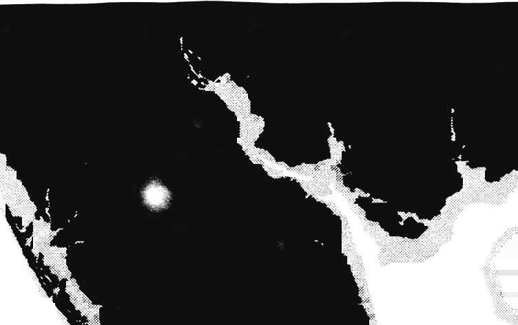
69 Figure10(d). Sightings of 'TSMD':

70 Figure10(e). Sightings of 'RPPR':

71 FigurelO(f). Sightings of 'LGSL':

72 Figure10(g). Sightings of TFLN':

73 Figure10(h). Sightings of 'elto':

74 Figure10(i). Sightings of 'ZIGV':

75 Figure10(j). Sightings of 'POTP':

76 Figure10(k). Sightings of 'DWf':

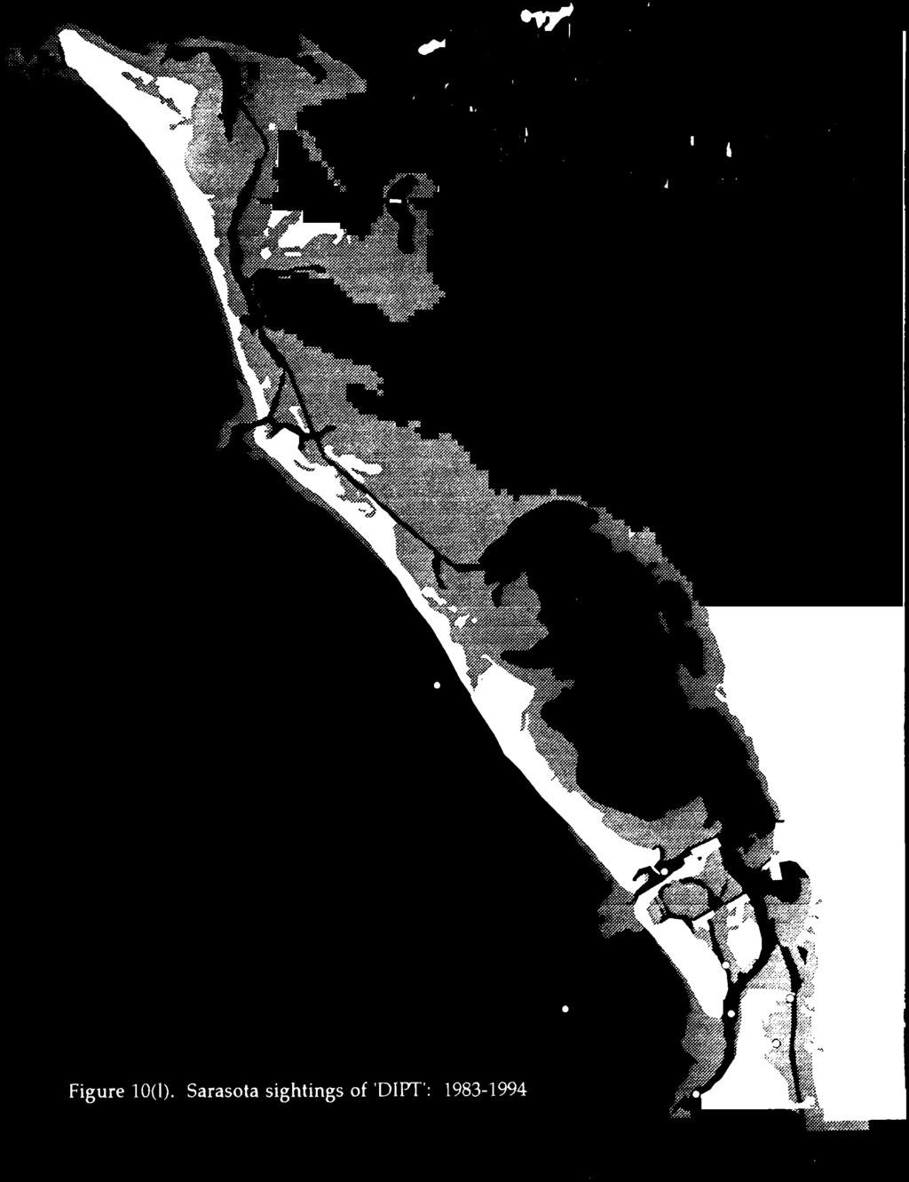
77 Figure 10(1). Sarasota sightings of 'OIPT:

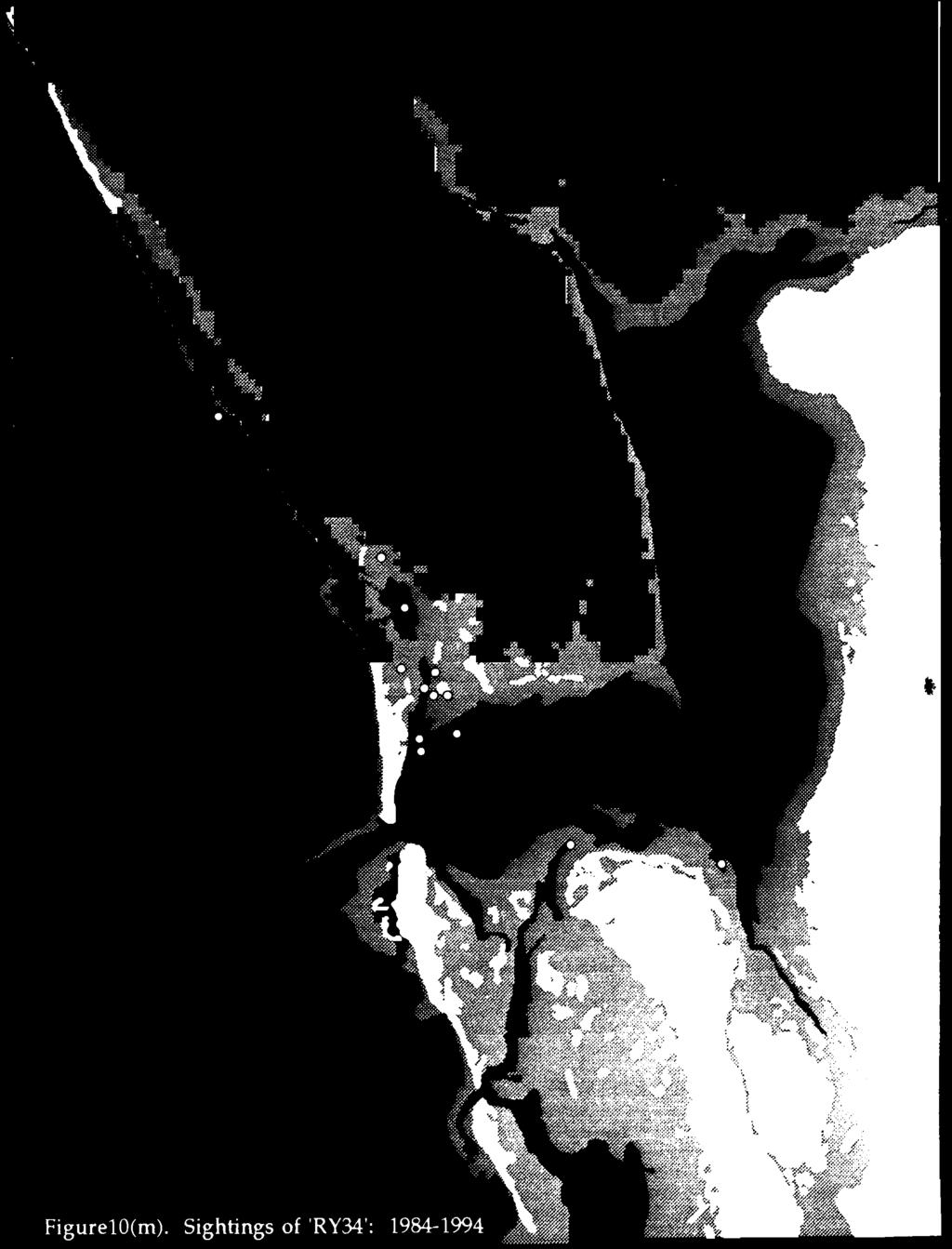
78 Figure10(m). Sightings of 'RY34':

79 Figure 10(n). Sarasota sightings of 'RY34':

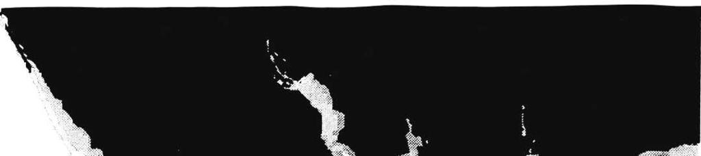
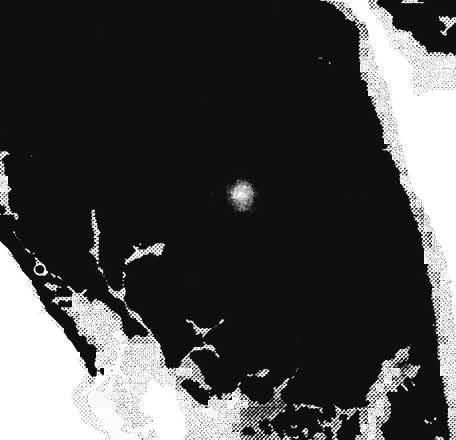
80 Figure10(o). Sightings of 'BSLC':

81 Figure 10(p). Sarasota sightings of 'BSLC:

82 Figure10(q). Sighting of 'SLIT: 16 August 1990

83 Figure10(q). Sighting of 'SLIT': 16 August 1990

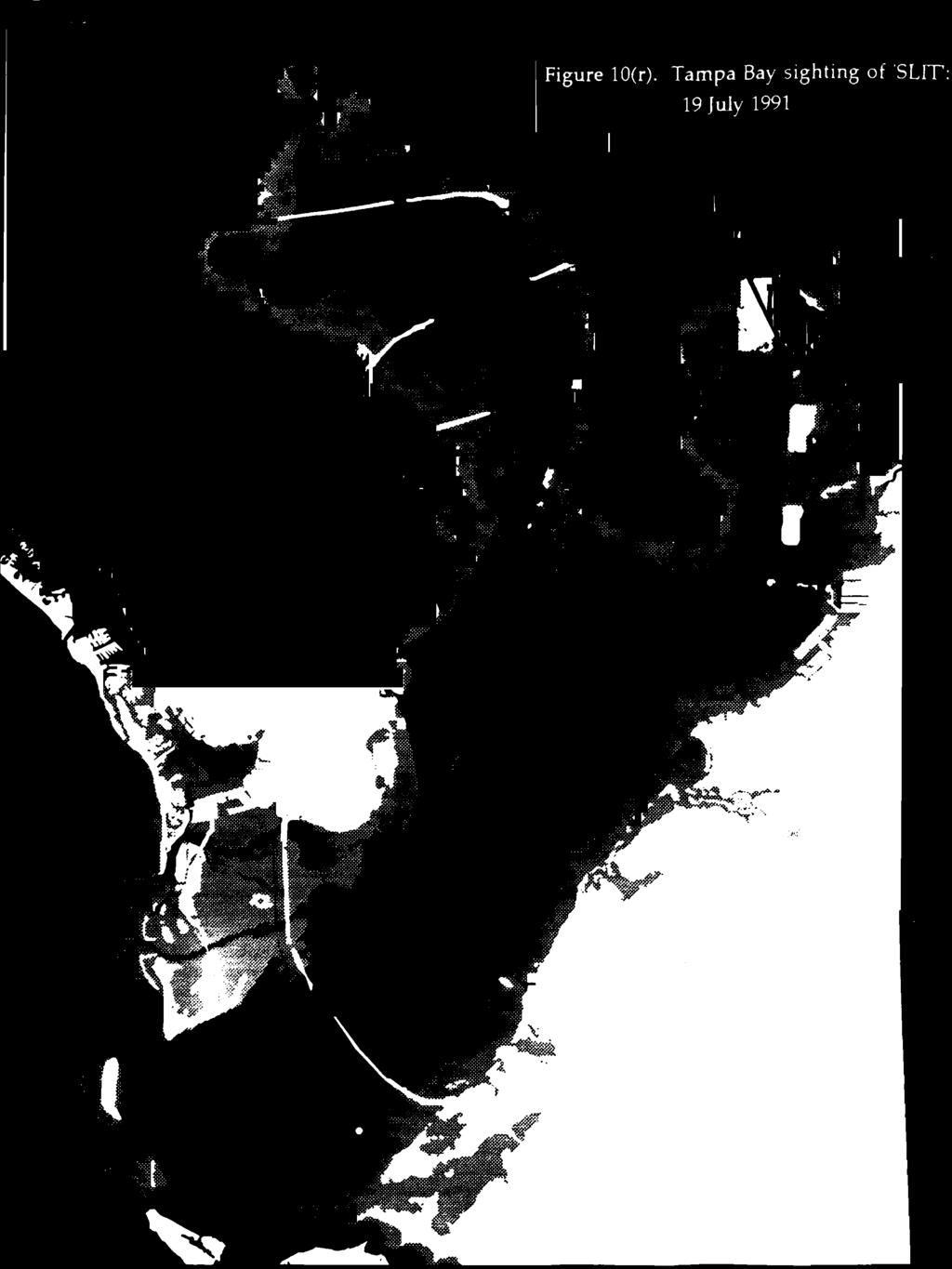
84 Tampa Bay sighting of 'SLIT': 19 July <

85 Dolphin Biology Research Institute Sighting Sheets Field Hours to _~ ~...;::~ Effort Is o C I D Date: Platform ~ S1g ht1ng No: D Observers Locat1on T1me : to LOC D Latitude I ~ ~~~~I ~1=~=~~I~I=~~~~I~~Lo-n-g-1t-u-de~I=~=~~I~I=~=~~I-I~~~~~I ~S~W~1m~s~pe ed 1,.' Condlt1ons CONDD Depth ~L~_~,=.~I-ft-. ~w-a-t-er~t-em~p:~i~~_=,=_~io~f~t-1-d-e:~~~n ~~~l J ~T=3~ H I~1 4~O=W~~H-e-a-d- 1 n-g-!~i=_=_~_~1 ~ Init ial General Act1vlty : Mill Feed Prob. Feed Travel Play Rest L eap Tallslap Ch uf f Soc i al w/boat Other I I _-_-_ FIE LD EST IM ATES TOTAL DOLPHI NS TOT AL CAL YES YOUNG OF YEAR Pos MIN MAX BEST IDs. PHOTO ANAL YS I S Max..not IOed Revl sed MIN Revl sed MAX I::] I::] I::]. 1::] \ 1::]..'. 1::]. "1::] I::] I::] I::] I::] 1::].... 1::] < 1::] < 1::].... I::] 1::]... 1::]... I::] I::] I::]. I::] C::1» 1::]... Final BEST Comments: Assoc1ated Organ1sms: Dolph1ns S1ghted: 10 confirmation: Nam e Code Conf. Name 1.==.1 1.==.1 1.==.1 1..=.1 1..= =..1 1.=..1 1.== P= photograph V= v1su al 0 = other (exol a1n) Code Conf. Name Code Con f. 1. I 1..I 1.== =_ ' 1._= ' 1. ' Photos: (roll: frame->frame) Tape: (tape: counter)

86 Appendix 1. Environmental condition codes. CONDITION CODES: SEA STATE WEATHER GLARE SIGHTABILITY Wave Height 0-0.2m (8 in) 0 Clear or few clouds 0 None 0 Excellent 0 Wave Height m (8-16 in) I Partly cloudy I Little, non- interfering I Good. unlikely to miss dolphins I Wave Height m (16-24 in) 2 Overcast 2 Some, could interfere 2 Fair, may miss some dolphins 2 Wave Height m (24-32 in) 3 Rain 3 Much. interfering 3 Poor, probably missing dolphins 3 Wave Height m (32-40 in) 4 Thunders torm 4 Not on effort 4 Wave Height > 1.0 m (>40 in) 5 Fog 5 INITIAL O R GENERAL HEADIN( : Use degrees in most cases, "360"=North Milling="OOO" In passes, rivers, us e "IN" or "OUT" if degrees are less appropriate