Durham E-Theses. The nature and timing of Late Quaternary glaciation in southernmost South America DARVILL, CHRISTOPHER

Transcription

1 Durham E-Theses The nature and timing of Late Quaternary glaciation in southernmost South America DARVILL, CHRISTOPHER How to cite: DARVILL, CHRISTOPHER (2015) The nature and timing of Late Quaternary glaciation in southernmost South America, Durham theses, Durham University. Available at Durham E-Theses Online: Use policy This work is licensed under a Creative Commons Attribution 3.0 (CC BY) Academic Support Oce, Durham University, University Oce, Old Elvet, Durham DH1 3HP e-theses.admin@dur.ac.uk Tel:

2 The nature and timing of Late Quaternary glaciation in southernmost South America Christopher Michael Darvill Department of Geography Durham University A thesis submitted in partial fulfilment of the requirements for the University of Durham for the degree of Doctor of Philosophy February 2015

3

4 The nature and timing of glaciation in southernmost South America Christopher Michael Darvill Abstract The timing and extent of former ice sheet fluctuations can demonstrate leads and lags during periods of climatic change and the forcing factors responsible, but this requires robust glacial chronologies. Patagonia, in southern South America, offers a well preserved record of glacial geomorphology over a large latitudinal range that is affected by key climatic systems in the Southern Hemisphere, but establishing the timing of ice advances has proven problematic. This thesis targets five southernmost ice lobes that extended from the former Patagonian Ice Sheet during the Quaternary; from north to south: the Río Gallegos, Skyring, Otway, Magellan and Bahía Inútil San Sebastián (BI-SSb) ice lobes. The region is chosen because there is ambiguity over the age of glacial limits, which have been hypothesised to relate to different glacial cycles over hundreds of thousands of years but yield cosmogenic nuclide exposure data dominantly < 50 ka. This contradiction is the focus of the thesis: was the sequence of glacial limits deposited over multiple glacial cycles, or during the last glacial cycle? A new geomorphological map is used to reconstruct glacial limits and to help target new dating. Cosmogenic nuclide depth-profiles through glacial outwash are used to date glacial limits whilst accounting for post-depositional processes. These reveal that limits of the BI-SSb lobe hypothesized to date from MIS 12 (ca. 450 ka) and 10 (ca. 350 ka) were actually deposited during the last glacial cycle, with the best-dated profile giving an MIS 3 age of ca. 30 ka, indicating an extensive advance prior to the global Last Glacial Maximum (glgm). A glacial reconstruction indicates that this may not have been unique to the BI-SSb lobe, and a compilation of published dates reveals that similar advances during the last glacial cycle indicate related forcing factors operating across Patagonia and New Zealand.

5 Resumen La datación y extensión de antiguas capas de hielo puede demostrar avances y retrocesos durante cambios climáticos así como factores responsables de esos cambios. Sin embargo, esto requiere de robustas cronologías glaciares. Patagonia, en el pico sur de Sudamérica, ofrece una buena preservación de la historia geomorfológica glaciar durante largas extensiones latitudinales, la cual es afectada por sistemas climáticos claves en el Hemisferio Sur, aunque el establecimiento de avances en las capas de hielo es problemático. Esta tesis tiene como objetivo estudiar cinco lenguas glaciares meridionales que se extendieron más allá de la capa de hielo que se formó en la Patagonia durante el Cuaternario. Estas son de norte a sur: El Río Gallegos, Skyring, Otway, Magellan y Bahía Inútil San Sebastián (BI-SSb). Esta región fue escogida debido a la ambigüedad sobre la datación de los límites del glacial hasta la fecha. Hipótesis señalan que estos límites pertenecen a diferentes ciclos glaciares durante cientos de miles de años pero a los que se les ha establecido una edad dominante de <50 Ka por medio de isótopos cosmogénicos. Esta contradicción es el centro de la tesis: fue la secuencia de límites glaciares depositada durante múltiples ciclos glaciares o durante el último ciclo glaciar? Un nuevo mapa geomorfológico ha sido elaborado para reconstruir límites glaciares y ayudar a establecer una nueva datación. Perfiles de los isótopos cosmogénicos a través de depósitos glaciares han sido utilizados para datar los límites del glaciar teniendo en cuenta procesos post-deposicionales. Estos revelan que los límites de la lengua glacial BI-SSb de supuesta edad de entre MIS 12 (ca. 450 ka) y 10 (ca. 350 ka) son en realidad depósitos del último ciclo glacial, donde la edad mejor definida se sitúa en el estadio isotópico MIS 3 (30 ka). Esto indica que antes del último periodo glacial máximo global hubo un extenso avance. La reconstrucción glacial indica que esta datación no es única de la lengua glacial BI-SSb, y una compilación de dataciones publicadas revela que similares avances durante el último ciclo glacial indican factores responsables de los cambios climáticos similares a través de Patagonia y Nueva Zelanda.

6 Contents Abstract... i Resumen... ii Contents... iii List of figures... x List of tables... xiv List of abbreviations... xv Declaration and statement of copyright... xvi Acknowledgements... xvii Chapter 1. Introduction Rationale Aims Research objectives Thesis structure and results Chapter Chapter Chapter Chapter Chapter Chapter 2. Study area and previous work Study area Previous work Nature of ice dynamics Glacial erosion and nested limits Ice flow dynamics Proglacial lakes Ice sheet modelling Timing of ice advances Drift characterisation Weathering analysis Argon-dating of basalts Amino-acid racemisation iii

7 Radiocarbon dating Uranium-series dating of marine terraces and glaciofluvial fans Palaeomagnetism Luminescence dating Cosmogenic nuclide exposure dating Terrestrial palaeoenvironmental reconstructions Vegetative reconstructions Dust records The Potrok Aike record Summary Chapter 3. A glacial geomorphological map of the southernmost ice lobes of Patagonia: the Bahía Inútil - San Sebastián, Magellan, Otway, Skyring and Río Gallegos lobes Introduction Study Area and Previous Work Previous Mapping Map production Imagery Geomorphological mapping Glacial geomorphology Moraine ridges Subdued moraine topography Kettle-kame topography Glacial lineations Irregular hummocky terrain Regular hummocky terrain Irregular dissected ridges Esker Meltwater channels Former shorelines Outwash plains Summary and conclusions Software iv

8 Chapter 4. Geomorphology and weathering characteristics of Erratic Boulder Trains on Tierra del Fuego, southernmost South America: Implications for dating of glacial deposits Introduction Definition and previous work on erratic boulder trains Formation: subglacial versus supraglacial Cosmogenic nuclide exposure dating This study Methods Mapping and sampling Size approximation, angularity, and appearance Schmidt hammer Profile gauge Results Distribution Volume characteristics Angularity Rock surface hardness Rock surface roughness Discussion Source Transport and deposition Rock surface weathering Alternative (post-)depositional model Conclusion Chapter 5. Extensive MIS 3 glaciation in southernmost Patagonia revealed by cosmogenic nuclide dating of outwash sediments Introduction Study area Methods Sampling Chemical analysis Age determination Scaling scheme and production rate Surface samples v

9 Depth profiles Previous exposure dating studies Results Surface sample results Depth profile modelling Sensitivity tests Density Inheritance Age limits Erosion rate Maximum erosion threshold Approach to modelling Depth profile modelling results Discussion New ages for BI-SSb glacial limits Geomorphic considerations Comparison with other southern mid-latitude studies Conclusions Chapter 6. The glacial history of five ice lobes in the southernmost Patagonian Ice Sheet Introduction Study area Methods Geomorphological mapping Glacial flowsets, limits and landsystems Proglacial lake reconstruction Results Moraine ridges Hummocky terrain Kettle-kame topography Glacial lineations Subdued moraine topography Irregular dissected ridges (IDR) Meltwater channels Outwash plains vi

10 6.4.9 Former shorelines Interpretation Glacial limits and flowsets Glacial landform assemblages Ice-marginal morainic landforms Subglacial landforms Glaciofluvial landforms Geometrical ridge landforms Palaeolacustrine landforms Discussion Active temperate glacial landsystem Other landform signatures Rapid ice flow Proglacial lake development Landsystem implications Glacial reconstruction Time step Time step Time step Time step Time step Time step Time step Time step Conclusions Chapter 7. Evaluating the timing and cause of glacial advances in the southern mid-latitudes during the last glacial cycle based on compiled exposure ages from Patagonia and New Zealand Introduction Methods Be dating compilation Radiocarbon dating Results Be chronology vii

11 7.3.2 Radiocarbon dating Relating 10 Be peaks to glacial advances Production rate and scaling scheme Surface erosion rate Inheritance Summary of peaks in timing Discussion The timing of glacial advances Comparison with other records Ice-rafted debris and dust records Other terrestrial records Possible forcing factors Insolation changes Ice core temperature changes Sea surface temperature changes Sea ice Upwelling Summary of last glacial cycle time periods Late MIS 5 (ca ka) MIS 4 (ca ka) Early MIS 3 (ca ka) Late MIS 3 (ca ka) MIS 2 (ca ka) and the glgm period ( ka) The late-glacial period (ca ka) Conclusions Chapter 8. Conclusions and implications Key conclusions Objective 1: Mapping of glacial limits Objective 2: Use of erratic boulder trains for dating Objective 3: Depth profile dating of key limits Objective 4: Reconstructing the regional glacial history Objective 5: Examining southern mid-latitude glaciation Implications Further work Dating of the Río Gallegos, Skyring and Otway lobes viii

12 Palaeo-Laguna Blanca drainage Ice thickness constraints Investigations into possible palaeo-surges Sedimentological work Dating pre-glgm moraines in Patagonia MIS 4 in Patagonia Ice sheet modelling References ix

13 List of figures Figure 1.1. Map of the southernmost Southern Hemisphere 3 Figure 2.1. Location of the study area in southernmost Patagonia 11 Figure 2.2. Illustration of the flow paths of the five former ice lobes 12 Figure 2.3. A section of the original glacial map Caldenius (1932) 13 Figure 2.4. Three of the original maps produced by Meglioli (1992) 17 Figure 2.5. Location of the area studied by Bujalesky et al. (2001) 23 Figure 2.6. The age ranges of all 10 Be analyses previously published for the study area 27 Figure 3.1. Location of the study area in southernmost Patagonia (topography shown using shaded SRTM and ETOPO data) 34 Figure 3.2. The location and previously hypothesised Marine Isotope Stage (MIS) chronology of drift limits within the study area 36 Figure 3.3. Overview of the study area showing the locations of other figures. Also shown is the area mapped by Lovell et al. (2011) 37 Figure 3.4. The spatial coverage of different imagery used during mapping 39 Figure 3.5. Aerial photograph and the mapped features in the central depression of the BI-SSb lobe 44 Figure 3.6. Kettle-kame topography on the northern edge of the BI-SSb lobe 45 Figure 3.7. Glacial lineations in the study area 46 Figure 3.8. Aerial photograph and mapped equivalent of the regular and irregular hummocky terrain 49 Figure 3.9. Landsat ETM+ image and mapped equivalent showing the intersection between lineations and irregular dissected ridges 50 Figure 4.1. Map showing the locations of erratic boulder trains 56 Figure 4.2. Maximum boulder diameter plotted against the maximum distance of boulders from their source lithology 58 Figure 4.3. The location of the study area, showing the extent of former ice lobes in southernmost South America 60 Figure 4.4. Simplified overview of the glacial geomorphology from Chapter 3 for Tierra del Fuego 60 Figure 4.5. Previous 10 Be cosmogenic nuclide exposure dates from the boulder trains 62 Figure 4.6. The different cosmogenic nuclide exposure dates from the boulders on Tierra del Fuego can be explained by two different hypotheses 64 x

14 Figure 4.7. Visualisation of the three methods used to calculate boulder volume from the same measurements 67 Figure 4.8. Photograph and illustration of the technique used to measure angularity of boulder edges 68 Figure 4.9. The profile gauge used to measure rock surface roughness 71 Figure Example photographs of the BI 1 boulder train, surface texture and boulders 73 Figure Example photographs of the BI 2 boulder train, boulders and surface texture 74 Figure Example photographs of the RC 1 boulder train and boulders 75 Figure The results of boulder volume measurements 77 Figure The results of angularity measurements 78 Figure Results of Schmidt hammer rock hardness analysis 79 Figure Results of profile gauge rock surface roughness analysis 80 Figure The rock surface hardness and roughness results plotted to illustrate variations in aspect with distance along the boulder trains 86 Figure 5.1. Location of the study area 92 Figure 5.2. The glacial geomorphology of the former BI-SSb ice lobe in Tierra del Fuego 95 Figure 5.3. Zoomed version of Figure Figure 5.4. Transects from Figure 5.3 showing the elevation change across the glacial drift limits and the sampled outwash 97 Figure 5.5. Panorama of the Filaret profile location 99 Figure 5.6. Photograph of the Filaret depth profile during sampling 100 Figure 5.7. Pictures of the surface cobble samples from the Filaret profile 101 Figure 5.8. Panorama of the Cullen profile location 102 Figure 5.9. Photograph of the Cullen depth profile during sampling 103 Figure Pictures of the surface cobble samples from the Cullen profile 104 Figure Cosmogenic nuclide results for the depth and surface samples 111 Figure Sensitivity tests for the 10 Be Filaret profile 115 Figure Sensitivity tests for the 10 Be Cullen profile 116 Figure Cullen 10 Be profile age, erosion rate and inheritance output for the 4 m maximum erosion model run 120 Figure Cullen 10 Be profile age, erosion rate and inheritance output for the 4 m maximum erosion model run 121 Figure Filaret 10 Be profile age, erosion rate and inheritance output for the 0.5 m maximum erosion model run 122 xi

15 Figure Filaret 10 Be profile age, erosion rate and inheritance output for the 0.5 m maximum erosion model run 123 Figure An illustration of how geomorphic effects would be expected to alter the relationship between measured surface sample nuclide concentrations and the modeled nuclide decay curve from depth samples 125 Figure Published dating of selected former ice lobe advances over the last 100 ka in Patagonia 127 Figure 6.1. Location of the study area in southern South America 132 Figure 6.2. Overview of the glacial geomorphology mapped in the study area 134 Figure 6.3. An overview of the glacial geomorphology associated with the Río Gallegos, Skyring, Otway and Magellan lobes 135 Figure 6.4. The IDR and drumlin field at the intersection of the Río Gallegos and Skyring lobes 137 Figure 6.5. Overview of the glacial geomorphology associated with the Magellan lobe 138 Figure 6.6. Overview of the glacial geomorphology associated with BI-SSb lobe 140 Figure 6.7. Enlarged portion of the central BI-SSb lobe geomorphology 142 Figure 6.8. A simplified version of the glacial geomorphology to show the dominant ice flow and ice marginal features 144 Figure 6.9. The dominant limits associated with four different sets of ice-marginal features 145 Figure Photographs and sketch of a section through the glaciotectonised moraine associated with re-advance of the Otway lobe 147 Figure Photographs and accompanying sketches of proglacially tectonised lacustrine silts and sands within an end moraine of the BI-SSb lobe 148 Figure Google Earth Image of the kettle and kame topography on the south side of the BI-SSb lobe 149 Figure The regular hummocky terrain from the centre of the BI-SSb lobe shown in a Google Earth image and crevasse-squeeze ridges in front of the surging Brúarjökull glacier in Iceland shown in a Microsoft Bing Maps image 152 Figure The evidence for palaeo-laguna Blanca and its drainage 155 Figure Rhythmically laminated sediments at Laguna Verde 156 Figure The glacial geomorphology of the central BI-SSb lobe and the Río Gallegos, Skyring, Otway and Magellan lobes, grouped according to the three landform assemblages indicative of an active temperate glacial landsystem 159 Figure Time step 1 and time step Figure Time step 3 and time step xii

16 Figure Time step 5 and time step Figure Time step 7 and time step Figure 7.1. Map of the Southern Hemisphere showing the positions of the Sub- Tropical Front, Sub-Antarctic Front and Polar Front, as well as the core region of the Southern Westerly Winds and the locations of ice and marine core records referred to in the text 178 Figure 7.2. The compilation of 10 Be and radiocarbon dates from Patagonia and New Zealand used in this study 181 Figure 7.3. Examining the effects of calculation parameters on the overall spread of ages in our compilation 183 Figure 7.4. Binned results from an analysis of skewness of probability density functions from individual moraine sets in Patagonia and New Zealand as a crude proxy for differential inheritance signatures 185 Figure 7.5. Orbital insolation parameters relevant to this study 191 Figure 7.6. A comparison of the timing of glacial advances in the southern midlatitudes during ka 194 Figure 7.7. As per Figure 7.6, but scaled to cover just ka. 194 xiii

17 List of tables Table 2.1. An overview of the drift deposits described and correlated by Meglioli (1992) 18 Table 3.1. Summary of the morphology, appearance and possible errors in mapping geomorphological features 39 Table 4.1. Summary of the key characteristics of EBTs based on a review of the literature 55 Table 4.2. Age and likely weathering characteristics for the Tierra del Fuego EBTs. 65 Table 4.3. Criteria used to visually assess boulder roundness (Benn, 2004). 67 Table 4.4. Angle corrections applied to Schmidt hammer R-values (Day & Goudie, 1977). 70 Table 4.5. The spatial characteristics and geomorphological context of the EBTs on Tierra del Fuego 72 Table 5.1. Sample descriptions and nuclide concentrations. 106 Table 5.2. Calculated ages for surface samples using CRONUS-Earth calculator (Balco et al., 2008) 107 Table 5.3. Details of comparison moraine boulder 10 Be chronologies from Patagonia for the last 100 ka 108 Table 5.4. Model parameters. 114 Table Be depth sample modelling summary 119 Table 6.1. The landforms expected in an active temperate glacial landsystem (adapted from Evans & Twigg, 2002; Evans, 2003) 158 Table 7.1. Details of the original works compiled in this study 179 Table 7.2. The timing of peaks in glacial advances identified from relative cumulative probability density functions for New Zealand and Patagonia 186 xiv

18 List of abbreviations AIM BI-SSb D-O EBT EDC EDML GLFC glgm/lgm GPG IDR IRD ITCZ m.a.s.l. MIS NGRIP PDF SAF SRTM SST STF Antarctic Isotope Maximum The Bahía Inútil San Sebastián ice lobe Dansgaard-Oeschger event Erratic Boulder Train EPICA Dome C ice core EPICA Dronning Maud Land ice core Global Land Cover Facility (global) Last Glacial Maximum Greatest Patagonian Glaciation Irregular Dissected Ridges Ice Rafted Debris Inter-Tropical Convergence Zone metres above sea level Marine Isotope Stage North Greenland Ice Core Project Probability Density Function Sub-Antarctic Front Shuttle Radar Topography Mission Sea Surface Temperature Sub-Tropical Front xv

19 Declaration and statement of copyright The copyright of this thesis rests with the author. No quotation from it should be published without the author s prior written consent and information derived from it should be acknowledged. I confirm that no part of the material presented in this thesis has previously been submitted by me or any other person for a degree in this or any other university. In all cases, where is relevant, material from the work of others has been acknowledged. Christopher Michael Darvill Department of Geography Durham University Submitted February 2015 Final version May 2015 xvi

20 Acknowledgements I am very grateful to my supervisors, Mike Bentley and Chris Stokes, whose guidance, patience and enthusiasm have helped me through my Ph.D., and whose insightful comments and accompaniment on fieldwork have contributed greatly to this thesis. Their equally good humour has also made the whole process great fun. I also owe a debt of gratitude to four friends who helped me as field assistants in Patagonia: Will Christiansen, Paul Lincoln, Harold Lovell and Mark Hulbert, the latter of whom also patiently helped me through much of the last three years. Thankyou all for your hard work and good company, and for putting up with me in the field! Many of the Durham Geography staff and postgraduate community have become good friends and provided a supportive community in which to conduct my research. There are too many people to name individually, but thanks to all those who have helped, listened or provided comic value in the office, GIS lab and coffee room. Ángel Rodés, Delia Gheorghiu, Alan Davidson and Andy Hein all gave up a lot of their time guiding me through the cosmogenic nuclide dating process and helping me to analyse my samples. Stefan Wastegård also kindly analysed some tephra samples for me, though I am sorry that they did not make the final thesis! Juan Carlos Aravena, Jorge Rabassa and Andrea Coronato were very generous with their time and assistance in Patagonia. Finally, to all of my great friends outside of Durham, to the Quatskis, and to my wonderful family Mum, Dad, Louise and Nick who have been so supportive and encouraging over the years, I thank my lucky stars you re all so brilliant. This thesis would not have been possible without the funding of a NERC studentship. My fieldwork and analyses also benefitted from funding by a number of other bodies. In chronological order, these are: an Explorers Club Exploration Grant; a QRA New Research Workers Award; the Durham University Faculty of Social Sciences and Health Projects and Initiatives Scheme; the Durham University Geography Department; NERC Cosmogenic Isotope Analysis Support (9127/1012; 9140/1013); a Santander Mobility Grant; a BSG Postgraduate Research Grant; an RGS Dudley Stamp Memorial Award; a Ustinov College, Durham Travel Award; and the Norman Richardson Postgraduate Research Fund. xvii

21

22 Chapter 1. Introduction 1

23 1.1 Rationale Southernmost South America is in a unique geographical position, heavily influenced by globally-important atmospheric and oceanic systems in the most southerly continental setting outside of Antarctica. However, despite the potential to improve our understanding of Southern Hemisphere and global climatic changes over multiple glacial cycles, the age constraints on the timing of pre-global Last Glacial Maximum (glgm) advances of former ice-lobes in the region remain poorly constrained. An improved chronology for the southernmost ice lobes of the former Patagonian Ice Sheet could yield important insights into climate variability at southernmost latitudes as well as processes governing long-term glacial dynamics. Just 2% of the earth s surface between 40 S and 60 S is land, mostly in southernmost South America (Zolitschka, 2009). These latitudes are dominated by the Southern Westerly Wind system (Figure 1.1), the strongest time-averaged oceanic winds in the world (Hodgson & Sime, 2010), which otherwise pass unhindered around the Southern Hemisphere. Southern South America is also fully exposed to changes in the Antarctic Circumpolar Current, a key component in the global oceanic circulation system. Both of these systems are thought to have a major influence on global climate: the Antarctic Circumpolar Current on the production of global deep-water (Corliss, 1983; Carter et al., 2008); and the Southern Westerly Winds on Southern Hemisphere precipitation, dust-fluxes and ocean-circulation (Kohfeld et al., 2013; Sime et al., 2013). Moreover, both are intrinsically linked by Antarctic (sea) ice extent and the positions of the oceanic frontal systems. Consequently, they are likely linked in their responses to climatic change (Boning et al., 2008; Wang et al., 2011). Terrestrial records at these latitudes can act as monitors of the strength of the Antarctic Circumpolar Current and latitudinal fluctuations of the Southern Westerly Winds and, by extension, changes within the Antarctic subcontinent and wider Southern Hemisphere (Sugden et al., 2005; Kaplan et al., 2008a). The location of southernmost South America, adjacent to the southern parts of the Atlantic and Pacific Oceans, means that the region may yield important insights into the contentious issue of inter-hemispheric climatic/glacial (a)synchrony (Broecker, 2003; Barker et al., 2009). Importantly, Patagonia is situated at the southernmost reaches of the former thermal bi-polar seesaw that may have operated in the Atlantic Ocean during periods of past climatic change. 2

24 Figure 1.1. Map of the southernmost Southern Hemisphere showing the Southern Westerly Wind System and Antarctic Circumpolar Current as well as oceanic frontal zones. Compiled from Carter (2009) and McGlone et al. (2010). 3

25 There is a rich terrestrial record in Patagonia, with Clapperton (1993) stating that: the combination of arid climate, successively less ice extent in each glaciation, and the large scale of the deposits, has preserved what is probably the most complete and intact sequence of Quaternary moraines anywhere in the world. (p. 352) However, there remains ambiguity regarding the timing of ice advances from what was once the southernmost part of the Patagonian Ice Sheet. In particular, the timing and nature of pre-glgm glacial advances is poorly understood. Without a comprehensive chronology of ice advances, it is difficult to appreciate how the different components of the land-ocean-atmosphere system fully interact during periods of climatic change (Lamy et al., 2007; Kaiser & Lamy, 2010). Significantly, if we are unsure of when glacial stages occurred in southernmost South America (e.g. at 30 ka or 1.1 Ma?), we cannot hope to properly calibrate regional and global models of climate, an essential step in effectively predicting future climate change. This problem is becoming more acute as longer ice core records are retrieved from Antarctica, spanning multiple glacial cycles (EPICA, 2004; 2006; 2010), that cannot be compared to terrestrial changes in Patagonia because of a lack of firm chronological control. This thesis focuses on constraining the timing of advances of five large ice lobes in the southernmost part of the former Patagonian Ice Sheet, from north to south: the Río Gallegos, Skyring, Otway, Magellan, and Bahía Inútil San Sebastián (BI-SSb) lobes. 1.2 Aims 1. To reconstruct glacial changes of the southernmost ice lobes of the Patagonian Ice Sheet, with a particular emphasis on glacial chronology, to determine whether ice advances occurred over timescales of 10 4, 10 5 or 10 6 years. 2. To use this new chronological framework to examine the controls on glacial change in southernmost South America. 4

26 1.3 Research objectives To address these aims, this work will be conducted through completion of five specific objectives: 1. Map the glacial geomorphology of southernmost South America from remote imagery and field-checking. 2. Examine the nature and weathering of erratic boulders that have yielded ambiguous cosmogenic nuclide dates on Tierra del Fuego. 3. Test the reliability of moraine boulder ages using a cosmogenic outwash depth-profiling approach. 4. Derive a glacial history for the region and assess the likely timing of glacial advances using previously published chronological information and new outwash depth-profile results. 5. Examine the trends in southern mid-latitude glaciation in order to explore ice sheet response to local, regional and hemispheric forcing. 1.4 Thesis structure and results Chapter 2 outlines previous work on the southernmost ice lobes of South America. Following this, Chapters 3-7 of this thesis are composed of a series of research papers that have been published, submitted, or prepared for peer-reviewed journals. An introduction to each chapter is given below. The papers have been edited for consistency within the thesis: introductory material has been reduced where necessary to avoid excessive repetition and supplementary information has been incorporated into the chapters where applicable. Because the methods used are specific to each chapter, they are included throughout the thesis rather than as a separate section. Chapters 3-6 present the analytical results and accompanying discussion of research conducted for this thesis to address Objectives 1-4 above. Chapter 7 incorporates this new research into a wider review and synthesis, discussing the likely climatic forcing mechanisms of southern mid-latitude glaciation and addresses Objective 5. Finally, Chapter 8 draws together the main conclusions of the thesis and explains how these address the aims outlined at the start. 5

27 1.4.1 Chapter 3 Darvill, C.M., Stokes, C.R., Bentley, M.J. & Lovell, H. (2014) A glacial geomorphological map of the southernmost ice lobes of Patagonia: the Bahía Inútil - San Sebastián, Magellan, Otway, Skyring and Río Gallegos lobes. Journal of Maps, 10, This paper outlines the methods and results of geomorphological mapping for the five southernmost ice lobes of the former Patagonian Ice Sheet. The centrepiece of the paper is a map that forms the basis for detailed analysis in subsequent chapters: contextualising the erratic boulder trains in Chapter 4; allowing targeted sampling of glacial limits in Chapters 5; and supporting the glacial reconstruction in Chapter 6. The map shows that meltwater landforms feature heavily in the region and reveals that limits associated with the Otway, Skyring and Río Gallegos lobes are marked by numerous clear moraine ridges, whereas the BI-SSb and Magellan lobes are marked by hummocky terrain and drift limits. The map also highlights cross-cutting landform relationships, suggesting multiple ice advances in those locations. In this paper, I undertook the mapping, wrote the manuscript and drew the figures. The map extended earlier work by Lovell for the Skyring and Otway area. All authors assisted with fieldwork, contributed ideas and edited the text. The paper has been published in Journal of Maps and the introduction has been edited for consistency Chapter 4 Darvill, C.M., Bentley, M.J. & Stokes, C.R. (2015) Geomorphology and weathering characteristics of erratic boulder trains on Tierra del Fuego, southernmost South America: implications for dating of glacial deposits. Geomorphology, 228, The interpretation of cosmogenic nuclide exposure dates from boulders associated with erratic boulder trains on Tierra del Fuego is a critical component in the argument for the age of glacial limits in the region. Previously reported ages have consisted of lots of younger ages (< 50 ka) with occasional older ages (> 50 ka), with the latter interpreted as closer to the true age, and the former attributed to erosion and exhumation. This paper conducts the first comprehensive study of these boulder trains, analysing their distribution, likely formation, and weathering characteristics to help contextualise the dating. The boulder trains are consistent with one or more supraglacial rock avalanches and weathering indices show little difference between them, suggesting that they could be much closer in age than previously thought. With this in mind, it is possible that occasional older cosmogenic 6

28 nuclide exposure dates result from an inheritance signature that was not removed by erosion during supraglacial transport, in which case the majority of younger dates are closer to the true age of deposition. In this paper, I undertook the fieldwork and analysis; wrote the manuscript; and drew the figures. All authors contributed ideas and edited the text. The paper has been published in Geomorphology and the supplementary information from that paper has been incorporated into the main text of this thesis Chapter 5 Darvill, C.M., Bentley, M.J., Stokes, C.R., Hein, A.S. & Rodés, Á. (in prep.) Extensive MIS 3 glaciation in southernmost Patagonia revealed by cosmogenic nuclide dating of outwash sediments. Earth and Planetary Science Letters. In the light of the hypothesis raised in Chapter 4, this paper provides the first age constraints for the San Sebastián and Río Cullen limits of the BI-SSb lobe in a way that is not compromised by exhumation and erosion processes. These pre-glgm glacial limits were previously hypothesised to date from Marine Isotope Stages (MIS) 12 and 10, but we demonstrate that they were deposited much more recently, during the last glacial cycle (MIS 4-2), including one clear MIS 3 advance. With this major reinterpretation of age, we suggest that the cause of such an extensive MIS 3 advance was most likely a southward shift of the Southern Westerly Winds, delivering greater precipitation to the ice lobe at a time of cooler summers and warmer, wetter winters. In this paper, I undertook the fieldwork, including sampling; much of the laboratory analysis; and most of the depth-profile modelling. I wrote the manuscript and drew the figures. All authors contributed ideas and edited the text. Bentley and Stokes assisted with fieldwork; Hein and Rodés assisted with depth-profile modelling; and Rodés assisted with laboratory analysis. The paper has been prepared for Earth and Planetary Science Letters, but the supplementary information has been incorporated into the main text and the introduction has been edited for consistency in this thesis Chapter 6 Darvill, C.M., Stokes, C.R. & Bentley, M.J. (in prep.) The glacial history of five ice lobes in southernmost Patagonia. Journal of Quaternary Science. This paper brings together new mapping of glacial geomorphology in southernmost South America from Chapter 3 with new age constraints on glacial limits from 7

29 Chapter 5 to present a new reconstruction of the timing and nature of glaciation in the region. We present a series of relative time steps based on our reconstructed glacial limits and, where possible, constrain the timing of glacial advances. In particular, we reinterpret previous chronological information in the light of our depthprofile dating campaign. All of the ice lobes are found to have displayed dynamic behaviour at times, with evidence for re-advances and the development of proglacial lakes that likely affected rates of advance and retreat. It is suggested that the Skyring, Otway and Magellan lobes were likely more extensive prior to the glgm, similar to findings in Chapter 5 for the BI-SSb lobe. In this paper, I undertook the analysis, wrote the manuscript and drew the figures. Stokes and Bentley contributed ideas, edited the text and assisted with fieldwork. The paper has been prepared for Journal of Quaternary Science Chapter 7 Darvill, C.M., Bentley, M.J. & Stokes, C.R. (in prep.) Evaluating the timing and cause of glacial advances in the southern mid-latitudes during the last glacial cycle based on compiled exposure ages from Patagonia and New Zealand. Quaternary Science Reviews. Chapters 5 and 6 demonstrated that southern ice lobes in Patagonia advanced prior to the glgm, and we argued that a similar pattern has emerged in other recent Southern Hemisphere studies, although it has not been widely discussed. In this paper, we compiled a large chronological dataset for Patagonia and New Zealand to compare the timing of regional ice advances and in so doing discuss the possible forcing factors behind Southern Hemisphere glacial advances during the last glacial cycle. We suggest that orbital parameters may underlie mid-latitude glacial activity, but that the migration of coupled ocean-atmosphere fronts, as part of a wider climatic feedback system, ultimately determines the timing of advances. In this paper, I undertook the analysis, wrote the manuscript and drew the figures. Bentley and Stokes contributed ideas and edited the text. The paper has been prepared for Quaternary Science Reviews. 8

30 Chapter 2. Study area and previous work 9

31 2.1 Study area The study area of this thesis focuses on the southernmost part of the former Patagonian Ice Sheet (Figures 2.1 and 2.2), specifically five ice lobes that extended eastward from the Andean Cordillera at times during the Quaternary period between around S. From north to south, these were the Río Gallegos, Skyring, Otway, Magellan and BI-SSb lobes. At present, only a handful of ice caps or small valley glaciers remain, principally the North Patagonian, South Patagonian and Darwin Cordilleran icefields (Figure 2.1). However, the glacial geomorphology of the former ice lobes is exceptionally well preserved by the relatively dry, arid climate and by the preservation of older geomorphology due to decreasing ice extents over time. Numerous up-to-date reviews exist which summarise the previous literature on glaciations in this region (Rabassa & Clapperton, 1990; Meglioli, 1992; Rabassa, 1992; Rabassa et al., 2000; Coronato et al., 2004; Rabassa et al., 2005; Rabassa, 2008; Rabassa et al., 2009; Rodbell et al., 2009; Coronato & Rabassa, 2011; Harrison & Glasser, 2011; Martínez et al., 2011; Rabassa et al., 2011; Kilian & Lamy, 2012). However, a critical assessment of the evidence for the timing of glaciations in southernmost South America is useful to highlight gaps in knowledge and issues associated with previous attempts at chronology. Early observations of the presence of glacial deposits in southernmost South America were made by Darwin (1841; 1845; 1848). Subsequently, Nordenskjöld (1899) was the first to accurately map glacial deposits in Patagonia, but it was Caldenius (1932) seminal work that defined the four glacial limits for Patagonia that are still broadly referred-to today (Figure 2.3). He named these deposits Initioglacial, Daniglacial, Gotiglacial and Finiglacial after the Swedish/European system, which implied that they were all of the last glaciation. It has since been shown that the older glacial limits were deposited more than a million years old (Meglioli, 1992; Ton-That et al., 1999; Singer et al., 2004a; Singer et al., 2004b; Hein et al., 2011). However, the original geomorphological characteristics of Caldenius system were built upon by Meglioli (1992) to establish the current conceptual model of glaciations for southernmost South America (Figure 2.2). This Regional Stratigraphic Model has since been used widely (Coronato et al., 2004; Rabassa, 2008; Coronato & Rabassa, 2011; Rabassa et al., 2011), although few of the glacial deposits have any absolute age controls. 10

32 Figure 2.1. Location of the study area in southernmost Patagonia, South America. The present day icefields (numbered) are shown as well as the hypothesised glgm, adapted from Singer et al. (2004a). 11

33 Figure 2.2. (A) Illustration of the flow paths of the five former ice lobes in the study area. (B) An overview of the place names mentioned in this chapter. (C) A conceptual diagram of the Regional Stratigraphic Model proposed by Meglioli (1992) showing the drift limits and their respective names for each lobe, as well as hypothesised age. See Table 2.1 for an overview of these drift deposits. 12

34 2.2 Previous work Nature of ice dynamics Glacial erosion and nested limits A decreasing extent of glacial limits over successive glaciations has been recorded at numerous locations in southern South America (the nested moraine formations observed in many glacial valleys; Caldenius, 1932; Figures 2.2 and 2.3). Kaplan et al. (2009) inferred that because these sequences do not match global climate variability, the decreasing ice extents cannot be linked to climate, and perhaps partly owe their origin to long-term erosional patterns, later modelled by Anderson et al. (2012). However, this hypothesis does not consider that the trends could be related to a regional (e.g. southern mid-latitude) climate trigger, which is not displayed by global climate records dominated by Northern Hemisphere signals. Figure 2.3. A section of the original glacial map of Patagonia by Caldenius (1932), cropped to the study area and with a key added to show his four proposed glacial stages. 13

35 Kaplan et al. (2009) suggested that over time, topographic changes (e.g. Jamieson et al., 2008) and changes in bedrock elevations (e.g. Montgomery, 2002) could jointly cause more negative glacier mass balances given a constant climatic forcing. In this way, the relationship between topography and Patagonian glacial extent is important to understand (Herman et al., 2013; Barr & Lovell, 2014), and may mask a climatic effect. To establish whether climate played a role, independent evidence is required to demonstrate that climatic changes occurred at the same time as glacier changes. For example, evidence of similar trends in glacial advances in other, distal locations at roughly the same latitudes would suggest that an external climatic forcing was responsible. These locations would need to be affected by similar atmospheric and oceanic systems for the argument to hold; ideal locations would be the glacier records of Patagonia and southern New Zealand (Figure 1.1) Ice flow dynamics There has been some work investigating the dynamics of ice advances and retreat in the study area. For example, numerous authors have mapped and commented on the spectacular drumlin field within the Otway lobe, around Laguna Cabeza del Mar (Clapperton, 1989; Clapperton et al., 1995; Benn & Clapperton, 2000b; Lovell et al., 2012; Figure 2.2), with Benn & Clapperton (2000b) suggesting it may have been formed by ice streaming. More recently, Lovell et al. (2012) presented a detailed reconstruction for parts of the Skyring, Otway and Magellan lobes, and found evidence for possible ice-streaming and surge-like behaviour. Although Benn & Clapperton (2000b) inferred a cold-based margin for the Magellan lobe, Bentley et al. (2005) and Lovell et al. (2012) suggested that this was unlikely. Recent bathymetric work has suggested that basal morphology, including tectonic controls, could have also played a role in defining ice extent in at least the Otway and Magellan lobes (Breuer et al., 2013) Proglacial lakes Numerous raised shorelines have been mapped in the study area, corresponding to all five southern ice lobes (Clapperton et al., 1995; McCulloch & Bentley, 1998; Bentley et al., 2005; McCulloch et al., 2005a; Glasser & Jansson, 2008; Lovell et al., 2011; Sagredo et al., 2011; Stern et al., 2011; Breuer et al., 2013; Kilian et al., 2013; De Muro et al., 2014; García et al., 2014). McCulloch et al. (2005a) and García et al. (2014) also presented detailed geomorphological and sedimentological evidence for proglacial lakes, as well as demonstrating post-glacial uplift of mapped shorelines due to isostatic and/or tectonic uplift. Recent work combining this evidence with 14

36 analysis of digital elevation models has provided some reconstructions of proglacial lake evolution that can supplement investigations into glacial advance and retreat (Lovell et al., 2012; Kilian et al., 2013; García et al., 2014). Porter et al. (1992), Clapperton et al. (1995), Bentley et al. (2005), McCulloch et al. (2005a), Lovell et al. (2012) and García et al. (2014) have commented on the formation and drainage of proglacial lakes in the region and the possible effects these had on ice dynamics. Porter et al. (1992) suggested that lakes in front of the Magellan and BI-SSb lobes may have increased the ice flow rate during recession, possibly even resulting in collapse. Similarly, Lovell et al. (2012) hypothesised that rapid flow of the Otway and Magellan lobes could have been linked to proglacial calving. However, the absence of evidence for ice-streaming in the Skyring lobe and for lake development in the Otway lobe makes it difficult to develop this argument further (Lovell et al., 2012) Ice sheet modelling Hulton et al. (1994) and Hulton et al. (2002) are the only studies to have modelled the entire Patagonian Ice Sheet, and this has provided useful insights into ice sheet dynamics and climatic forcing. For example, the modelling highlighted the marked contrast between the east and west of the ice sheet. However, this ice sheet-scale modelling has not been updated to include more recent insights into chronology and modelling power (e.g. compared to Golledge et al. (2012) for New Zealand). One of the reasons for this is the challenging nature of modelling the Patagonian Ice Sheet. It covered a long latitudinal range (and therefore north-south temperature gradient) and experienced differing regimes from west to east (Hulton et al., 2002; Sugden et al., 2002). On the western side of the ice sheet, glaciers were dominantly marineterminating, not reaching far from the Andean range but receiving high rates of precipitation carried by westerly winds from the Pacific Ocean. In contrast, the eastern side was relatively drier but was terrestrial terminating, with large ice lobes travelling far from the mountains (Coronato et al., 2008; Rabassa, 2008). Furthermore, Kerr & Sugden (1994) demonstrated a strong dependence of former glaciers on temperature changes, but also that the southern part of the ice sheet was particularly sensitive to precipitation. Uncertainty in changes in the delivery of precipitation by the Southern Westerly Winds, which may have migrated or expanded north and southward over time, makes it challenging to model the former ice sheet. Finally, Glasser & Jansson (2005) also noted that ice streaming within 15

37 parts of the ice sheet may help to explain why matching model outputs to the geomorphological record has proven so challenging. Nonetheless, modelling the whole ice sheet is important because more localised studies of individual glacier systems become limited by assumptions about ice-flow dynamics or chronological constraints that are ultimately difficult to answer without taking a broader, ice sheet-scale view. For example, studies such as Hubbard et al. (2005) for northern Patagonia and Fernandez et al. (2011) for the Marinelli glacier system in Cordillera Darwin offer a level of detail that may be missed by a coarser model, but struggle to ascertain whether glacier fluctuations are linked to external climate forcing or internal flow dynamics. There is great capacity for further modelling of the Patagonian Ice Sheet, though it is beyond the scope of this thesis Timing of ice advances For this introductory chapter, previous dating of glacial limits is reviewed using the data and interpretations as originally stated in the published works. However, for techniques such as radiocarbon dating and cosmogenic nuclide exposure dating, there have been recent advances in age calibration and so, on subsequent use in the rest of the thesis, dates are re-calibrated where relevant. Whilst a range of dating techniques have been applied to glacial limits in the study area, these have been conducted and interpreted according to the Regional Stratigraphic Model by Meglioli (1992; Table 2.1). Numerous glacial drift deposits have been assigned relative stratigraphic ages in the region, which are thought to broadly correspond between ice lobes (Coronato et al., 2004). This is supported by relative weathering ages and a few absolute ages from intervening volcanic deposits (Meglioli, 1992). There has been lots of subsequent work on the younger, inner drifts, which date from around the glgm (Coronato et al., 2004; Coronato & Rabassa, 2011; Rabassa et al., 2011), but little work on the older, outer drifts. An important argument in the age of the older drifts is that marine terraces can be linked to glacial limits (Bujalesky et al., 2001). However, a key geomorphic relationship has not been evidenced and dates on the marine terraces are themselves problematic. Most recently, work using cosmogenic nuclide exposure dating of boulders gave a spread of ages that were interpreted in light of the Regional Stratigraphic Model, such that a small number of relatively old ages were taken as closest ages for the drifts (Kaplan et al., 2007; Evenson et al., 2009). Given the complexity in these arguments, it is worth examining the evidence in detail. 16

38 Figure 2.4. Three of the original maps produced by Meglioli (1992) to illustrate his characterisation of drifts across the study area, with a key added to show his hypothesised age model Drift characterisation The Regional Stratigraphic Model for southernmost South America proposed by Meglioli (1992) is based upon drift characterisation (Figure 2.4) and consists of isolated examples of the Rio Grande drift followed by local representations of the Greatest Patagonian Glaciation (GPG, ca. 1.1 Ma; Mercer, 1976), then three subsequent glaciations (Coronato et al., 2004) before the glgm (Clapperton et al., 1995; McCulloch et al., 2005b; Table 2.1). The drifts were defined by Meglioli (1992) based on the relationship of outwash deposits to moraines; moraine morphology; boulder frequency and weathering; presence or absence of cryogenic features; and some were also dated using weathering rind analysis and 40 Ar/ 39 Ar dating of basalts. For simplicity, these drifts are referred to as glacial limits throughout the following Chapters and local names are used where necessary to avoid correlation without actual age constraints. 17

39 18 Table 2.1. An overview of the drift deposits described and correlated by Meglioli (1992), along with glaciation names, weathering rind ages, robust argon dates (where available) and hypothesised MIS chronology, whereby MIS 2 corresponds to the glgm. Grey shading indicates the GPG drifts. Río Gallegos lobe drifts Skyring lobe drifts Otway lobe drifts Magellan lobe drifts BI-SSb lobe drifts Glaciation Weathering rind age (ka) 40 Ar/ 39 Ar ages (ka) MIS Río Grande??? Bella Vista Pali Aike Pali Aike Sierra de los Frailes Pampa de Beta Sierra de los Frailes 1200 ± 200 ca ? Glencross Rio Zurdo Rio Ciake Cabo Vírgenes Río Cullen Cabo Virgenes 450 ± Laguna Blanca Dinamarquero Punta Delgada San Sebastián Punta Delgada 10 Rio Turbio Rio Verde Oazy Harbour Primera Angostura Lagunas Secas Primera Angostura 140 ± Seno Almirante Montt Seno Skyring Seno Otway Segunda Angostura Bahía Inútil Segunda Angostura 15.8 ± 0.2 2

40 Weathering analysis Meglioli (1992) conducted weathering analysis at 87 sites across the study area, which was used as the principal justification for assigning the different drifts to separate glacial cycles. Some important points should be made regarding the spatial distribution of these analyses. First, the Río Gallegos, Skyring and Otway lobes are distinctly underrepresented by analyses, with only 18 of the total 87 sites within these lobes. Secondly, within the Magellan and BI-SSb lobes, the distribution of sites between drifts is unequal. For example, the Lagunas Secas drift is only represented by one sampling location (correlated with a further fifteen on the Primera Angostura drift). While Caldenius (1932) also recorded a distinct glacial limit ( Las Morenas de Filaret, assigned to the Gotiglacial), this is the only dated sample from the Lagunas Secas drift. Finally, the precise positioning of some of the drift limits has large implications for the weathering results, even though Meglioli (1992) observed that the separation of some drifts was unclear. These issues are necessarily guided by the availability of suitable sampling sites, and are not problematic if one assumes that the correlation between lobes can be made. However, Meglioli (1992) also made it clear that calibration of the weathering rind age model was highly tentative. Of the four points that were used in the construction of a weathering rind calibration curve, one had an age range based on a distal argon date from northern Patagonia assumed to be equivalent in age (140 ka in Table 2.1) and two have large age ranges dictated by argon dates from capping lava flows (450 and 1200 ka in Table 2.1). Thus, the calibration curve has large age errors, though these are not necessarily clear from the age estimates presented in the Regional Stratigraphic Model Argon-dating of basalts Argon-dating (including K-Ar and 40 Ar/ 39 Ar dating) of volcanic deposits capping drift sediments underpins much of the Regional Stratigraphic Model. Meglioli (1992) used 40 Ar/ 39 Ar dating of lava flows to constrain the ages of drifts north of the Magellan Straits and improve the chronology of Mercer (1976). The age of the Sierra de los Frailes drift (Figure 2.2 and Table 2.1) was constrained to between 1.4 ± 0.1 and 1.07 ± 0.03 Ma based on basalt flows below and above the drift, respectively. Furthermore, the Cabo Virgenes drift (Figure 2.2 and Table 2.1) was bracketed by the second basalt flow at 1.07 ± 0.03 Ma and a further overlying flow dated to 450 ± 10 ka. However, relating the dated tills to glacial limits is not necessarily straightforward. 19

41 Subsequent studies by Ton-That et al. (1999) and Singer et al. (2004a) improved the dating of Meglioli (1992) for the Bella Vista drift in the Río Gallegos depression. The accepted age for this drift is now ± Ma (Singer et al., 2004a), confirming mapping of the greatest glacial extent in Patagonia by Caldenius (1932) and the GPG proposed by Mercer (1976), now regionally bracketed to between and Ma Singer et al. (2004a). The exact relationship between the Río Gallegos lobe, the Skyring lobe and the Bella Vista drift is less clear, although it is usually presumed that the two ice lobes coalesced, such that the drift date corresponds to both (Rabassa, 2008). There are no argon dates relating specifically to the BI-SSb lobe Amino-acid racemisation Amino-acid racemisation analysis has been conducted on marine shells in the study area, although no analyses have been conducted in the Río Gallegos, Skyring or Otway lobes. Work by Rutter et al. (1989) and Meglioli (1992) has been cited as providing age constraint on glacial drifts of the BI-SSb lobe, but is actually related to raised marine terraces, and the former makes no connection between these and drift deposits. In contrast, Clapperton et al. (1995) and McCulloch et al. (2005b) presented analyses of shells from tills within moraines of the Magellan lobe relating to their Advances A (pre-segunda Angostura drift) and B/C (Segunda Angostura drift). Combined with radiocarbon dates, shells from the Segunda Angostura drift imply a marine incursion occurred in the Magellan Strait around 35 ka, linked to considerable deglaciation and implying that the Magellan lobe could have advanced during MIS 4 or earlier (Clapperton et al., 1995). However, there are a number of assumptions associated with the calibration of the amino-acid racemisation analyses and they do not provide absolute ages (Clapperton et al., 1995) Radiocarbon dating Radiocarbon dating has been applied across the study area. Due to its limited applicable age span, the technique has been most useful in constraining ice fluctuations from the glgm onwards. For example, Sagredo et al. (2011) and Stern et al. (2011) recorded ice recession and proglacial lake development from at least ca cal ka BP in the Río Gallegos lobe, following deposition of the Seno Almirante Montt drift. Subsequent re-advances may then have occurred before 16.2 cal ka BP and around cal ka BP (Sagredo et al., 2011). The Skyring and Otway lobes contain few radiocarbon dates, dominantly from marine cores within their respective sounds. In Seno Skyring, the oldest radiocarbon 20

42 age of 12.9 cal ka BP and the Reclus tephra age of ca cal ka BP support an age model that implies ice retreat before ca. 18 ka. Similarly, the oldest age from Seno Otway is ca cal ka BP, with an accompanying age model suggesting ice retreat before ca. 17 ka. This is consistent with a date of >14.2 cal ka BP for the abandonment of an overspill channel from the Otway proglacial lake into the Strait of Magellan (Mercer, 1976; McCulloch et al., 2005a; Kilian et al., 2013). The Magellan and BI-SSb lobes have been analysed extensively using radiocarbon dating of the Segunda Angostura and Bahía Inútil drifts. Shell samples from beyond the Segunda Angostura drift limit in the Magellan lobe, likely relating to Primera Angostura and Punta Delgada drift, were dated by Porter (1990) and Clapperton et al. (1995). The infinite ages were suggested to show that these drifts were deposited > 47 ka, and possibly during MIS 4 or earlier. However, McCulloch et al. (2005b) later suggested that the dates indicated a prolonged opening of the Strait of Magellan to the Pacific Ocean, and therefore any MIS 4 advance would have been less extensive than the glgm. McCulloch et al. (2005b) also synthesised a large number of radiocarbon dates from shells and organic material within moraines and lacustrine sediments from the Magellan and BI-SSb lobes, along with cosmogenic nuclide exposure dates, and suggested three ice advances using their glacial stages: at ca cal ka BP (Stage B), before ca cal ka BP (Stage C) and before ca cal ka BP (Stage D). The compilation also reconstructed relatively rapid deglaciation following these advances and a re-advance during the Antarctic Cold Reversal. However, recent radiocarbon dating by Hall et al. (2013) implies ice retreat well into Cordillera Darwin by ca cal ka BP, significantly earlier than proposed by McCulloch et al. (2005b). These dates seem to be supported by a marine core from the Marinelli Fjord within the Cordillera (Boyd et al., 2008), but are controversial because radiocarbon dating and tephrochrological analyses indicate that proglacial lakes existed in the Strait of Magellan and Bahía Inútil until ca cal ka BP (McCulloch & Bentley, 1998; McCulloch et al., 2000; McCulloch & Davies, 2001; McCulloch et al., 2005a; McCulloch et al., 2005b) Uranium-series dating of marine terraces and glaciofluvial fans A key piece of evidence for the ages of BI-SSb lobe drifts is the relationship between marine terraces and glaciofluvial fans on the east coast of Tierra del Fuego (Coronato et al., 2004; Rabassa, 2008; Coronato & Rabassa, 2011; Rabassa et al., 2011). Bujalesky et al. (2001) analysed three raised beach formations, and dated 21

43 them using Uranium-series analysis on shells within the terraces (Figure 2.5). These marine terraces are inferred to represent three marine transgressions, strongly implying that they were formed during (at least) three successive interglacials. If they can be linked geomorphologically to any of the drifts, therefore, they can be used as evidence for the separation of the drifts into different glaciations. 22

44 Figure 2.5. (A) Location of the area studied by Bujalesky et al. (2001), with their mapping shown in (B) and (C), adapted from the original figures. The lower glaciofluvial terrace is shown in brown in both (B) and (C). (D) is a conceptual diagram to illustrate the relationship between dated marine terraces, glaciofluvial terraces and drifts proposed by Bujalesky et al. (2001). 23

45 Two glaciofluvial terraces were also described by Bujalesky et al. (2001) as corresponding to the Río Cullen and San Sebastián drift limits (Figure 2.5), although there is no direct chronological evidence for their ages. The lower terrace has been eroded by the three marine terrace formations, suggesting that it formed prior to three marine transgressions. Crucially, the geomorphic link to the glacial limits was not described by the authors. The dating on the Las Vueltas and Laguna Arcillosa marine terraces (Figure 2.5) is uncertain given that a portion of the Uranium-signature of both samples implied terrestrial rather than marine origin. Weathering had occurred so that lack of contamination and a closed-system could not be guaranteed, particularly for the Las Vueltas sample. Bujalesky et al. (2001) suggested that issues of weathering and contamination affecting the Laguna Arcillosa samples would most likely lead to an age of >400 ka and <600 ka; and that the Las Vueltas age is probably unreliable given weathering and terrestrial contamination. The Las Vueltas terrace was only assigned an age of <300 ka based on dating and the stratigraphic position of the terrace. Coronato & Rabassa (2011; p.723) stated that based on the stratigraphical position of paraglacial fans and raised marine beaches, Bujalesky et al. (2001) postulated that the Sierras de San Sebastián and Lagunas Secas glacial limits should correspond to MIS 10 and 6, respectively. However, this link is not straightforward because: 1. There is no independent dating of the Lagunas Secas drift and there is no definitive evidence to show that it formed in a separate glacial stage. 2. There is no geomorphic link between the raised marine terraces and the Bahía Inútil or Lagunas Secas drifts with the raised beach formations. 3. The correlation of the San Sebastián drift with MIS 10 is based on the assumption that it was a separate glacial stage, older than the Lagunas Secas drift (presumed MIS 6) and younger than the Río Cullen drift. MIS 10 was selected by Coronato et al. (2004) and Coronato & Rabassa (2011) based on Uranium-series dating of the Las Vueltas formation, despite the fact that this dating is stated as being uncertain (Bujalesky et al., 2001). Given that the age of the Lagunas Secas drift is unknown, there is no reason why the San Sebastián drift cannot be of MIS 6 age or younger. 24

46 4. The system of three raised beach formations only incise the lower glaciofluvial fan, hypothesised to link to the Río Cullen drift (Bujalesky et al., 2001). This suggests that deposition of the Río Cullen drift was followed by three interglacial marine transgressions, the oldest of which was likely >400 ka and the youngest of which was at ca. 82 ka (MIS 5). However, this does not provide an absolute age for the Río Cullen drift, or any ages for the San Sebastián and Lagunas Secas drifts. Crucially, there is no evidence given to demonstrate that the glaciofluvial fans relate to the San Sebastián and Río Cullen drifts Palaeomagnetism Walther et al. (2007) presented palaeomagnetic results from glacial sediments from northern Tierra del Fuego. Analysis of basal till from the Río Cullen drift exposed at Bahia San Sebastián demonstrated that it formed during the normally-polarised Brunhes chron and that the Río Cullen, San Sebastián and Lagunas Secas drifts formed after 760 ka (Walther et al., 2007; Rabassa et al., 2011). No similar palaeomagnetic studies have been conducted for the Río Gallegos, Skyring, Otway or Magellan lobes Luminescence dating Luminescence dating has only been successfully used once in the study area, with Blomdin et al. (2012) obtaining an age of around 22 ka for the deglaciation of the Brunswick Peninsula area west of the Strait of Magellan, supporting the radiocarbon dating chronology in that location (McCulloch et al., 2005b). More important than the age estimates, their study, like that of Harrison et al. (2008) in northern Patagonia, highlighted the need to use alternative techniques to Optically Stimulated Luminescence (OSL) dating of glacial sediments in Patagonia. Blomdin et al. (2012) utilised K-Feldspar Infrared Stimulated Luminesce (IRSL), whereas Glasser et al. (2006) and Harrison et al. (2012) used single grain OSL dating. No luminescence dating has been conducted on the Río Gallegos, Skyring and Otway lobes, but the technique has great potential to help constrain glacial limits in the study area in the future Cosmogenic nuclide exposure dating No cosmogenic nuclide dating has been published on deposits relating to the Otway or Skyring lobes, but the Río Gallegos lobe has been dated using 10 Be and 36 Cl analysis of erratic boulders. The Bella Vista drift was dated to 47 ka and 106 ka, with 25

47 both ages substantially younger than expected (Kaplan et al., 2007). Likewise, the Rio Turbio and/or Glencross drifts yielded five dates of ka (Evenson et al., 2009; the exact sampling strategy is unclear from their work). Sagredo et al. (2011) dated younger limits of the Río Gallegos lobe (which they refer to as the Última Esperanza lobe) using four boulders which yielded ages of ka. There are issues of stratigraphic consistency within the combined cosmogenic nuclide exposure ages for the Río Gallegos lobe, and tying these ages to glacial drifts or limits is challenging. The Magellan lobe has been dated using 10 Be and 26 Al analysis. For the Segunda Angostura drift, the ages are consistent with the glgm, as previously hypothesised (Meglioli, 1992; McCulloch et al., 2005b; Kaplan et al., 2007; Kaplan et al., 2008a). However, eight dates from the Primera Angostura, Punta Delgada and Cabo Vírgenes drifts yielded young ages <133 ka, with the six dates from the Primera Angostura drift yielding ages of ka. This is a similar situation to cosmogenic nuclide exposure dating of the BI-SSb lobe. Erratics boulder trains within the southern margin of the BI-SSb lobe have been dated extensively by a number of studies, with those on the southern side of Bahía Inútil supporting other dating techniques and assigning the Bahía Inútil drift to the glgm (McCulloch et al., 2005b; Kaplan et al., 2007; Kaplan et al., 2008a; Evenson et al., 2009). Kaplan et al. (2007) also measured combinations of 10 Be, 26 Al and 36 Cl nuclides on erratic boulder trains from pre-glgm limits within the BI-SSb lobe. They found that on the Rio Cullen and San Sebastián drifts (assumed to be >350 ka) erratics showed relatively young exposure ages (generally <50 ka; Figure 2.6). In light of the Regional Stratigraphic Model (Meglioli, 1992; Coronato et al., 2004), Kaplan et al. (2007) proposed that episodic exhumation and erosion of the vast majority of the boulders during the glgm had caused anomalously young ages, and that the oldest ages were closest to the true age of glacial advance. This was supported by the large range of cosmogenic nuclide exposure ages compared to other ice lobes in northern Patagonia (Kaplan et al., 2004; Douglass et al., 2005; Kaplan et al., 2005; Douglass et al., 2006). Evenson et al. (2009) presented a further twenty 10 Be and 36 Cl cosmogenic samples for the BI-SSb lobe. There is little discussion of the analyses, but they suggested that the Laguna Secas drift may have been deposited during MIS 4, rather than MIS 6, and that wave-washing may have occurred during isostatic depression following MIS 4. Conversely, Evenson et al. (2009) also pointed out that excessive boulder erosion is unlikely to have occurred at the same rate on all boulders over hundreds of thousands of years, thus 26

48 producing relatively tightly clustered ages. Kaplan et al. s (2007) explanation for the spread of cosmogenic ages is logical and is not contradicted by the Evenson et al. (2009) results. However, it is based on fitting to the Regional Stratigraphic Model, which presumes that dating prior to cosmogenic nuclide exposure analysis was robust and the ages of the limits were relatively well known. This chapter has highlighted that independent age-constraint of the drifts prior to cosmogenic nuclide exposure dating was not as robust as suggested and that the interpretation of the cosmogenic ages may be worth revisiting. Figure 2.6. The age ranges of all 10 Be analyses previously published for the study area (see text for details). Dates are labelled according to the drifts (and hypothesised ages according to the Regional Stratigraphic Model) to which they relate. 27

49 2.2.3 Terrestrial palaeoenvironmental reconstructions Previous studies have demonstrated links between glacial activity in southern South America and wider past environmental changes. This section briefly outlines a selection of the terrestrial reconstructions from the study area, focussing on pre- Holocene records. These can be used to help interpret glacial activity, but may also be affected by new insights into the timing of glacial activity in the area Vegetative reconstructions Markgraf (1993) used pollen records from across southernmost South America to show the succession of vegetation change towards Nothofagus forest into the Holocene. This was later supplemented by D/H stable isotopic analyses to improve the temperature and moisture reconstructions, suggesting increased precipitation after ca. 15 cal ka BP (Pendall et al., 2001). Heusser (1993; 1995; 2003) and Heusser et al. (2000) also reconstructed vegetation changes along the Strait of Magellan, demonstrating that tundra-like vegetation (e.g. Empetrum and Acaena) existed during the late glacial, consistent with a cooler, drier climate. The pollen record of McCulloch & Davies (2001) supported this, suggesting warming and retreat of the Magellan lobe from ca cal ka BP but cooler temperatures until ca cal ka BP. They also suggested that a period of cooler and drier climate during ca cal ka BP altered vegetation composition at the same time as an ice re-advance during the Antarctic Cold Reversal. In the Skyring lobe, Kilian et al. (2007) showed a shift towards Magellanic Rainforest in the region after ca. 11 cal ka BP, possibly indicative of the end of a similar Antarctic Cold Reversal in this ice lobe. Markgraf (1993), Heusser (1995) and Pendall et al. (2001) all noted the importance of the Southern Westerly Winds in determining vegetation spread. More recent work on post-late glacial pollen records has also suggested a link between environmental changes and the wind system, possibly invoking the Southern Annular Mode (Moreno et al., 2009a; Moreno et al., 2010; Moreno et al., 2012; Moreno et al., 2014), but using pollen records in this way to reconstruct changes in winds intensity may be problematic (Kohfeld et al., 2013) Dust records Patagonia is one of the dominant sources of southern hemispheric dust found in Antarctic ice-core records (Kaiser & Lamy, 2010; McGee et al., 2010; Wolff et al., 2010a; Martinez-Garcia et al., 2011). Sugden et al. (2009) demonstrated a 28

50 theoretical and geochemical link between glacial activity in southern South America (including the Magellan lobe), dust availability, and pre-warming dust deposition in Antarctic ice-cores. They suggested that as glaciers retreated in Patagonia, large outwash plains were exposed, and became sources of atmospheric dust which is preserved in Antarctic ice cores (Fischer et al., 2007). Importantly, as ice retreated into proglacial lakes, the dust source was effectively switched-off, explaining an early reduction in Antarctic dust compared to global temperature rise after ca. 20 ka (Sugden et al., 2009). It is possible that dust resulting from fluctuations of Patagonian glaciers was one of the major drivers of Quaternary global climatic change (Lambert et al., 2008) The Potrok Aike record The Potrok Aike Maar lake is situated within the study area, to the east of the Río Gallegos lobe and north of the Skyring lobe, and deserves special mention because it has been the subject of intense study over the last five years (Zolitschka, 2009; Recasens et al., 2012; Zolitschka et al., 2013). The lake is suggested to have remained stable and relatively free of glacial and glaciofluvial activity over the last ca. 800 ka (Coronato et al., 2013), though a core record has been shown to cover only ca. 51 ka (Buylaert et al., 2013; Kliem et al., 2013b; Lisé-Pronovost et al., 2013; Wastegård et al., 2013). Nonetheless, this record has been used to reconstruct changes in a variety of palaeoevironmental parameters, including lake level (Kliem et al., 2013a) and Southern Westerly Wind intensity (Lisé-Pronovost et al., 2014; Zhu et al., 2014; Lisé-Pronovost et al., 2015), and transfer functions for pollen and diatoms have been developed from around 16 ka to aid palaeoenvironmental and climatic reconstructions (Massaferro & Larocque-Tobler, 2013; Schäbitz et al., 2013). Many of these proxies are still in the developmental stages, but recent work using stable isotopes (Zhu et al., 2014) and mineral magnetic properties (Lisé- Pronovost et al., 2015) over the last 51 ka may help to show how the Southern Westlery Wind system operated during periods of significant climatic change. It is likely that the Potrok Aike site will yield further invaluable environmental and climatic information for the study area in the future. 2.3 Summary There has been much work on the reconstruction of glacial dynamics in southernmost South America, but there remain several key issues that would benefit from further investigation. Of particular interest are the causes for reduced glacial extent over time (Kaplan et al., 2009; Anderson et al., 2012) and the possibility of 29

51 highly dynamic ice lobes (Lovell et al., 2012). However, without understanding the time frame within which the ice lobes advanced, it is difficult to fully assess the nature of glacial change. There is significant uncertainty in the age of glacial limits in the study area. Meglioli (1992) proposed the Regional Stratigraphic Model of four drifts deposited after the GPG (Caldenius, 1932; Singer et al., 2004a). Weathering rind data was used to separate these drift deposits into four different glacial cycles (Meglioli, 1992). The age of the GPG has been well constrained by Meglioli (1992), Ton-That et al. (1999) and Singer et al. (2004a) using argon-dating of basalts capping the Bella Vista drift of the Río Gallegos lobe to ca. 1.1 Ma. Porter (1990) and Clapperton et al. (1995) provided infinite radiocarbon ages for the Punta Delgada and Primera Angostura drifts of the Magellan lobe and Rutter et al. (1989), Meglioli (1992), Clapperton et al. (1995) and McCulloch et al. (2005b) used amino acid racemisation analysis to suggest that the Primera Angostura drift of the Magellan lobe formed prior to the glgm. The glgm is well constrained for the Magellan and BI-SSb lobes (and, to an extent the Río Gallegos lobe) by a variety of chronological techniques. There are few, if any, firm age constraints for pre-glgm limits in the region, and large uncertainty surrounds those of the BI-SSb lobe. Bujalesky et al. (2001) suggested that the Rio Cullen drift of the BI-SSb lobe may have formed the lower of two glaciofluvial terraces eroded by three raised marine terraces, which would imply that the Rio Cullen drift was followed by at least three interglacial cycles, although this link is ambiguous. Cosmogenic nuclide exposure dating by Kaplan et al. (2007) and Evenson et al. (2009) produced scattered dates, but dominantly < 50 ka. However, dates from limits older than the glgm limit were called into question because they did not fit the Regional Stratigraphic Model. This leads to an important, but not previously discussed observation. Specifically, there is at least as much chronological evidence to suggest that the glacial limits deposited after the GPG, but before the glgm, were part of an earlier advance during the last glacial cycle, as there is to suggest that they were from several previous glacial cycles. Clearly, robust age constraints from these limits are required, and this is a key motivation for this thesis. These may then have important implications for the interpretation of other palaeoenvironmental and climatic records in southernmost South America. 30

52 Chapter 3. A glacial geomorphological map of the southernmost ice lobes of Patagonia: the Bahía Inútil - San Sebastián, Magellan, Otway, Skyring and Río Gallegos lobes Darvill, C.M., Stokes, C.R., Bentley, M.J. & Lovell, H. (2014) A glacial geomorphological map of the southernmost ice lobes of Patagonia: the Bahía Inútil - San Sebastián, Magellan, Otway, Skyring and Río Gallegos lobes, Journal of Maps, 10,

53 Abstract This paper presents a glacial geomorphological map of the landforms created by five large ice lobes that extended eastwards from the southernmost reaches of the Patagonian Ice Sheet during the Quaternary period. The study is focussed on Tierra del Fuego, but also updates previous mapping of the Skyring and Otway lobes, and the resulting level of detail and extent is a significant advance on previous work in the region. The map has been created as the necessary precursor for an improved understanding of the glacial history of the region, and to underpin a programme of dating glacial limits in the region. It was produced using Landsat ETM+ and ASTER satellite imagery and vertical aerial photography, supplemented by Google Earth imagery and field-checking. Eleven landform types were mapped: moraine ridges, subdued moraine topography, kettle-kame topography, glacial lineations, irregular and regular hummocky terrain, irregular dissected ridges, eskers, meltwater channels, former shorelines and outwash plains. The map reveals three important characteristics of the glacial geomorphology. First, the geomorphic systems are largely dominated by landforms associated with meltwater (channels, outwash plains and kettle-kame topography). Second, there is a difference in the nature of landforms associated with the northern three ice lobes, where limits are generally marked by numerous clear moraine ridges, compared to those to the south, where hummocky terrain and drift limits prevail. Finally, cross-cutting landforms offer evidence of multiple advances, in places, which has implications for the timing of limit deposition, and thus for the design and interpretation of a dating programme. 32

54 3.1 Introduction Patagonia contains some of the longest and best-preserved records of glaciation in the world (Clapperton, 1993). Contemporary glaciation in the region is restricted to three ice caps: the North and South Patagonian and Cordillera Darwin Icefields (Figure 3.1). However, it has been demonstrated that these advanced and coalesced at various times during the Quaternary, as part of an extensive Patagonian Ice Sheet centred on the southern Andes (Caldenius, 1932; Meglioli, 1992; Coronato et al., 2004; Glasser et al., 2008; Rabassa, 2008). Given its location in a region heavily influenced by important atmospheric and oceanic circulation systems, such as the Southern Westerly Winds and the Antarctic Circumpolar Current, Patagonia has received increasing attention in recent decades because it may yield insight into the mechanisms of climatic change in the Southern Hemisphere (Ackert et al., 2008; Kaplan et al., 2008a; Moreno et al., 2009b; Strelin et al., 2011; Murray et al., 2012; Boex et al., 2013) and help in understanding interhemispheric glacial (a)synchrony (Moreno et al., 2001; Sugden et al., 2005; García et al., 2012). Combined with the numerous palaeoenvironmental records that now exist across Patagonia, the timing and pattern of glacial changes may be used to infer changes in past climate (Sugden et al., 2005; Kilian & Lamy, 2012; Moreno et al., 2012). Extending these investigations beyond the glgm, however, has thus far proven problematic for the southernmost parts of the region. This is partly due to the lack of a comprehensive mapping of glacial landforms at an appropriate scale (> 30 m resolution) and coverage (regional rather than local), and partly due to uncertainties in existing chronological data (Kaplan et al., 2007). As such, the aim of this paper is to produce a comprehensive map of the glacial geomorphology deposited by the southernmost ice lobes of the Patagonian Ice Sheet that builds on and extends previous work in terms of detail and coverage (Section ). The map is designed to enable a refined reconstruction of the glacial history of the region using glacial inversion techniques (Kleman et al., 2006) and will be used as the foundation for dating glacial limits in the area, particularly the enigmatic pre-glgm limits that have thus far proven contentious. 33

55 Figure 3.1. Location of the study area in southernmost Patagonia (topography shown using shaded SRTM and ETOPO data). Also shown are the present day icefields (numbered) and the Last Glacial Maximum (glgm) limit according to Caldenius (1932); adapted from Singer et al. (2004a). 34

56 3.1.1 Study Area and Previous Work Previous Mapping This mapping focuses on an area into which the five southernmost ice lobes (the BI- SSb, Magellan, Otway, Skyring and Río Gallegos lobes; Figure 3.2) advanced from the main Patagonian Ice Sheet. Previous work suggests that these lobes were substantially more extensive compared to others in Patagonia (Caldenius, 1932). Early work by Nordenskjöld (1899) and Bonarelli (1917) suggested that Patagonia had been previously glaciated possibly several times but it was the seminal work of Caldenius (1932) that first extensively mapped the glacial geomorphology of the region and suggested that several different stages of glaciation were recorded by the nested nature of the geomorphological limits. Subsequently, there have been several studies that have built upon this early mapping. Raedecke (1978) produced a geomorphological map of the Chilean side of the BI-SSb lobe. It highlighted the complex nature of the geomorphology, describing thrust and en echelon moraines as well as bands of drift deposits, but the extent of mapping was limited to the central depression of the BI-SSb lobe. In contrast, Meglioli (1992) mapped the surface features of the southernmost ice lobes at a much broader scale. The study focussed on drift and soil characterisation rather than glacial landforms, resulting in a map which could be considered a representation of surficial properties, rather than depicting glacial landforms. Nonetheless, this work established the current conceptual model for the pattern and timing of glaciations in the region using both relative and absolute dating techniques (Figure 3.2) and was summarised in Coronato et al. (2004). More recently, Glasser & Jansson (2008) produced an extensive geomorphological map of the whole Patagonian region. However, the nature of such large-scale mapping meant that the resolution was necessarily coarse and some of the subtle complexity in the geomorphology of individual ice lobes was not recorded. In contrast to Glasser & Jansson s (2008) map, small regions of the hypothesised glgm geomorphology in the study area have been mapped in detail by Clapperton et al. (1995), McCulloch & Bentley (1998), Benn & Clapperton (2000b), Bentley et al. (2005) and Sagredo et al. (2011). Bujalesky et al. (2001) also mapped an area of older glaciofluvial fans to the south of Bahía San Sebastián and Coronato et al. described the geomorphology surrounding the Aike maar, east of the Río Gallegos lobe. Additionally, Ercolano et al. (2004) described a drumlinised area within the Río Gallegos valley of the Río Gallegos lobe. 35

57 Lovell et al. (2011) produced a map of the glacial geomorphology within the Otway and Skyring lobes region (area shown in Figure 3.3). It was the most detailed map produced of the area and was subsequently used to interpret the glacial dynamics of the ice lobes, including surge-like advances and the development of pro-glacial lakes during retreat (Lovell et al., 2012). Figure 3.2. The location and previously hypothesised Marine Isotope Stage (MIS) chronology of drift limits within the study area (Meglioli, 1992; Rabassa et al., 2000; Singer et al., 2004a). 36

58 Figure 3.3. Overview of the study area showing the locations of other figures. Also shown is the area mapped by Lovell et al. (2011), with red boxes highlighting the key areas that have been updated. 3.2 Map production The map was produced using a combination of remote sensing analysis and fieldchecking, with multiple types (and resolutions) of imagery consulted to provide a rigorous interpretation of the glacial geomorphology (Figure 3.4). The central BI-SSb area is shown in an enlarged inset to help improve the clarity of the geomorphology in this lobe, which is substantially more complex than in the other lobes. A copy of this map can be found in the Appendix Imagery Across the region, Landsat ETM+ scenes from the Global Land Cover Facility (GLFC; were used for mapping. These cover an area of km and have a spatial resolution of 30 m (or 15 m in band 8). Landsat imagery was supplemented by Google Earth imagery (version 7, available from consisting of 2013 Cnes/SPOT images and 2013 DigitalGlobe images (up to ~5-15 m resolution). ASTER images from the NASA 37

59 Land Processes Distributed Active Archive Centre ( were also used. These cover an area of km, with a spatial resolution of 15 m. Aerial photographs were used in preference to satellite imagery, where available, and revealed significant complexity that had been missed from some previous maps. A total of 76 vertical aerial photographs were used (12 digital with ~5 m resolution; and 64 scanned hard copies with ~8 m resolution; both from the Servicio Aerofotométrico del la Fuerza Aérea de Chile; Figure 3.4). Where aerial photographs were not available, Google Earth often provided imagery of only slightly lower resolution. Shuttle Radar Topographic Mission (SRTM) data (3 arcsec data, 90 m resolution) from the GLFC depository were used to identify some features only visible as subtle changes in topography and to provide topographic context as a shaded relief greyscale background to the map. Field seasons during 2012 and 2013 allowed cross-checking of features mapped from remote imagery, although it was not possible to cover the entire area in detail (~80,000 km 2 ) so fieldwork focused on key mapping elements (Figure 3.4). The study area includes an area around Seno Skyring and Seno Otway that was previously mapped by Lovell et al. (2011; Figure 3.3), and their mapping is included and updated here for two reasons. Firstly, not doing so would leave a large gap in the final geomorphological map, making it difficult to assess the complete geomorphology across the region. Similar mapping criteria and styles have been adopted here as in Lovell et al. (2011) to maintain consistency across the entire area. Secondly, extensive field-seasons in 2012 and 2013 have allowed fieldchecking of the previous work for the first time, and we have updated the mapping based on this (Figure 3.3). 38

60 Figure 3.4. The spatial coverage of different imagery used during mapping. Inset shows the approximate area in which field-checking was conducted. Spatial (pixel) resolution of the different imagery is given in the key. Table 3.1. Summary of the morphology, appearance and possible errors in mapping geomorphological features. The visibility of features on different imagery is also indicated: plus signs mean that features are normally visible; minus signs mean that features may sometimes be visible; and no sign indicates that features are not normally visible on the imagery. 39

61 40 SRTM Landsat ASTER Aerial scans Aerial photos Field Identification criteria Visibility Incr. resolution Landform Morphology Appearance Uncertainties Moraine ridges Distinctive linear or curvilinear ridges deposited at the ice margin or in medial positions. Arcuate ridges of positive relief (indicated by darker/lighter shading on opposing sides). Often, following the direction of fragmentary ridges leads to the identification of further features. Medial moraines could have been missed as they would be particularly difficult to identify under these criteria. Ridges and shorelines could potentially be confused. Often only visible in aerial photos Subdued moraine topography Similar to ridges but much wider and with lower elevations, and break-ofslope not as clear. Subtle changes in topography, with or without change in surface texture, which may be overprinted by more distinct features. Sometimes visible in the field and on SRTM data, very occasionally visible on aerial photographs or Landsat imagery. Almost certainly missed where ground-truthing was not possible or where they were not visible on SRTM. Difficult to pick-out on the ground and very difficult to identify from imagery Kettle-kame topography Large belts consisting of disorganised hills and hollows. Distinctive areas with a pock-marked appearance, consisting of hills and sometimes small lakes. May contain ridges. Can become discontinuous in lower areas associated with outwash. Sometimes difficult to distinguish drift from terrain that has simply avoided meltwater. Texture can vary significantly (with the presence of kettle lakes, the shape of hills) Glacial lineations Linear, parallel landforms aligned to the direction of ice-flow. Linear features following the inferred direction of ice-flow and generally perpendicular to moraines, often occurring in groups. Not specifically associated with breaks in vegetation and often appear dark on one side and light on the other, indicating positive relief. Can be short and consequently difficult to identify, even on aerial photos (often invisible on Landsat/ASTER). Fence lines could be mistaken for lineations, and the features are often disrupted by small lakes or (melt)water drainage Irregular hummocky terrain Areas of small, disorganised hills. Subtle patches of hills showing no obvious order and only visible in aerial photography. Only visible on aerial photographs, and therefore could have been missed in areas with no coverage. The boundaries of the hummocky areas can be difficult to discern

62 41 Regular hummocky terrain Irregular dissected ridges Eskers Meltwater channels Former shorelines Outwash plains Groups of small hills, elongated into small ridges and mirroring patches of small moraine ridges. Groups of larger hills or constrained areas of higher relief, sometimes delineated by minor meltwater channels. Sinuous ridges, generally running sub-parallel to former ice flow. Channels formed by large amounts of water from melting ice, often not containing contemporary drainage. Raised terraces marking the previous level of a body of water (either sea-level or a lake). Large areas of material deposited by meltwater in a flattened, grading plain. Extremely subtle and only visible on high-resolution aerial photography. Order is in the apparent form of several hummocks joined into a small ridge. These very short ridges are difficult to discern in the field without the aid of the aerial photography. Patches of raised topography, often marked by changes in surface texture or vegetation. Sometimes show a mosaiclike pattern, divided by meltwater channels. Sinuous ridges showing a change in colour due to the shadowing caused by positive relief. Generally sinuous in form and often occurring in combination with moraine ridges, running against contemporary slope. Frequently do not follow modern drainage routes or contain modern drainage, though this is not universal. Normally parallel to the coast or an area occupied by a lake and forming concentric lines without relief on one side (shown by shading). Shoreline level is either flat or grades evenly along its length. Large, open, approximately flat surfaces, grading to a previous ice limit (marked by moraine ridges, drift, etc), and often dissected by meltwater channels. Generally distinguished by a clear block change in colour and texture on Landsat imagery. Will be missed in areas not covered by highresolution aerial photography. The organised nature frequently becomes apparent only once numerous ridges have been mapped. Drainage can sometimes give the illusion of ridges. Actual changes in topography are often difficult to see in imagery, so identification can become overreliant on vegetation changes. Difficult to identify. Moraine ridges, lineations (especially when deformed) or meltwater channels could be mistaken for eskers. Often filled with contemporary drainage even though fieldwork has demonstrated they are oversized and were once filled with or created by meltwater. Often discontinuous and may become difficult to see when their direction changes, particularly in satellite imagery. May be missed where the location of a palaeo-lake is unknown, and difficult to distinguish from moraine ridges. Exact limits of outwash are often difficult to define. Surface grading is often only apparent in the field or over large distances on SRTM. Often form narrow corridors, so can be difficult to distinguish from channels Lakes Bodies of water surrounded by land (with no link to the sea). Blue, black or white in colour imagery; white or black in monochrome. Clearly delimited areas often linked to local drainage. Where transient, can show eastward migration patterns linked to westerly winds. Not always obvious in aerial photos (a counterpart photo is sometimes necessary). Extent of many lakes is very seasonally variable so their size can vary in different imagery and in the field Volcanic craters Hollows formed by volcanic eruptions. Rounded or elliptical and generally creating linear fields. Unlikely to be mistaken for glacial geomorphology

63 3.2.2 Geomorphological mapping In total, eleven different glacial features were mapped as line and/or polygon symbols using ArcMap 10 software: moraine ridges, subdued moraine topography, kettle-kame topography, glacial lineations, irregular hummocky terrain, regular hummocky terrain, irregular dissected ridges, eskers, meltwater channels, former shorelines, and outwash plains. Lakes and prominent volcanic craters were also mapped to provide landscape context and because these systems have been used in previous dating studies in the region. 3.3 Glacial geomorphology The glacial geomorphological features mapped in this study are summarised in Table 3.1 in terms of their morphology, appearance and any uncertainties in their identification Moraine ridges Moraine ridges are linear or curvilinear, elongate features exhibiting positive relief. They may be level-crested or undulating, continuous or fragmentary, but are distinguished by their linearity and consistency with formerly expanded ice margins. In places, they may overprint lineations (Section 3.3.4) and subdued moraine topography (Section 3.3.2; Figure 3.5), and can coincide with areas of kettle-kame topography (Section 3.3.3) and irregular hummocky terrain (Section 3.3.5). Ridges are often discontinuous, and it is rare to find complete lateral-terminal moraine systems, with the exception of the Otway lobe, where continuous ridges run for tens of kilometres. These features range from small, fragmentary crested ridges, often up to a few hundred metres long and less than 10 metres high (only visible on aerial photography and in the field in the BI-SSb and Magellan lobes; Figure 3.5), up to larger, continuous or semi-continuous hilly ridges, which are up to tens of kilometres long and tens of metres high, such as those delineating the Skyring and Otway lobes. Much of what Glasser & Jansson (2008) mapped as moraine ridges in the BI-SSb and Magellan lobes, we map as hummocky terrain or kettle-kame topography because they form wide areas of hilly terrain rather than narrow elongate ridges. This is likely due to a difference in mapping criteria and resolution of imagery used, which may also help explain differences in mapping between Glasser & Jansson (2008) and Lovell et al. (2011). There is generally good agreement between our mapping and that of Clapperton (1995), McCulloch & Bentley (1998), Benn & 42

64 Clapperton (2000b), Bentley et al. (2005) and Coronato et al. (2013) who all worked at a higher spatial resolution Subdued moraine topography These are somewhat elusive features, occurring mainly in the BI-SSb lobe, but also in the Río Gallegos lobe. They exist as subtle changes in relief, generally not more than 10 metres high and up to a kilometre wide, which are parallel to the orientation of moraine ridges. The features are distinguished as vegetation changes in some places on Landsat imagery and/or very low-relief changes on SRTM data and fieldobservations helped to confirm their existence. North of Laguna Larga, in the BI-SSb lobe, the moraines exhibit regular fragmentation (Figure 3.5). The subdued moraines are significantly broader than moraine ridges and are not sharp-crested. Likewise, they are very low relief and low gradient, and are thus unlike hummocky terrain. It is suggested that both moraine ridges and hummocky terrain may be overprinted on the subdued moraines (Figure 3.5). These features do not seem to have been mapped previously Kettle-kame topography Kettle-kame topography is common within the BI-SSb and Magellan lobes. Unlike moraine ridges, the drift constitutes wide bands (often > 2 km) of an irregular mixture of hills and hollows, some containing small kettle-lakes. The kame hills can be greater than 10 m high and rarely show any regularity in their arrangement. Other studies have depicted these deposits as moraine ridges (Clapperton et al., 1995; McCulloch & Bentley, 1998; Bentley et al., 2005; Glasser & Jansson, 2008), which is understandable given that the drift and ridges both record ice advance limits. However, we here follow Raedecke (1978) and Benn & Clapperton (2000b) in mapping the drift as a distinct feature given its clarity in imagery and on the ground. It is particularly prominent as two large, distinctive belts within the BI-SSb lobe (Figure 3.6), forming the Rio Cullen and San Sebastian drift limits of Meglioli (1992; previously mapped by Caldenius, 1932). 43

65 Figure 3.5. (A) Aerial photograph and (B) the mapped features in the central depression of the BI-SSb lobe. Thin, low moraine ridges (mapped as purple lines) are indicated by the black arrows and drape across the subdued moraine topography (mapped as pink polygons) and lineations (black lines). Locations shown in Figure 3.3. (C) Field photograph of one of these moraine ridges draped over subdued moraine topography; location shown in (A) and (B) by black circle with arrow. (D) Field photograph of the larger moraines in the Skyring lobe, separated by expansive outwash. Heights in metres above sea level (m.a.s.l.) are shown for the moraines and outwash plain. 44

66 Figure 3.6. Kettle-kame topography on the northern edge of the BI-SSb lobe. (A) Landsat ETM+ (bands 4, 3, 1) showing the characteristic pock-marked appearance of the drift. (B) Mapped bands of drift (purple polygons), separated by outwash surfaces (yellow polygons). Location shown in Figure Glacial lineations Glacial lineations form beneath an ice sheet and are aligned with ice flow direction (Clarhäll & Jansson, 2003). They occur frequently throughout the study area, from scattered and subdued flutings (< 1m high) to tightly constrained clusters of classic oval-shaped drumlins tens of metres high (Figure 3.7). Where the break of slope could be readily identified, lineations were mapped as polygons, but this was only possible in localised, well-defined drumlinised areas, centred around the Skyring and Otway lobes (Lovell et al., 2011). Elsewhere, and particularly in the BI-SSb lobe, the lineations are mapped as lines. Raedecke (1978), Benn & Clapperton (2000b), and Glasser & Jansson (2008) also mapped lineations but identified fewer features. For example, we map a significant number of lineations within the BI-SSb lobe, which overlie subdued moraine topography and are cross-cut by moraine ridges. Ercolano et al. (2004) noted a swath of elongated drumlins within the Río Gallegos lobe geomormorphology, but did not map them individually. 45

67 Figure 3.7. Glacial lineations in the study area. (A) Aerial photograph showing a tightly clustered field of low-relief flutings on the coast of Bahía Inútil and (B) the flutings mapped as black lines. Shorelines are also shown running parallel to the coast (light blue lines). The circle and arrow in (A) show the direction of the field photograph in (C), looking across the flutings which have been highlighted with white lines; locations shown in Figure 3.3. At the other end of the scale, (D) shows a field photograph of the much larger, sharp-crested drumlins in the Laguna Cabeza del Mar field of the Otway lobe (see map) Irregular hummocky terrain We present two forms of hummocky terrain in the study area (irregular and regular), and opt for this nomenclature rather than hummocky moraine (Lukas, 2005; Graham et al., 2007; Lukas, 2007) or controlled moraine (Evans, 2009) to avoid genetic inference. In the field, the hummocky terrain appears as patches of small, semirounded hills, rarely more than five metres high (and often less) and ten metres across. Irregular hummocky terrain is significantly more extensive than the regular version (Section 3.3.6) and lacks an organised pattern (Figure 3.8). Raedecke (1978) mapped these features in some parts of the BI-SSb lobe as kettle-kame deposits, forming semi-lobate areas in the centre of the depression. We distinguish hummocky terrain from kettle-kame topography (Section 3.3.3) on the basis of a significant difference in scale, highlighted by the difference in visible resolution (Table 3.1) and a general lack of obvious kettle-holes. Similarly to Raedecke (1978), 46

68 we also mapped a semi-lobate pattern, and we also note that the feature is exclusive to the BI-SSb lobe Regular hummocky terrain Regular hummocky terrain is rare in the study area and consists of two or three small interconnected hills, forming ridges transverse to ice-flow (Figure 3.8). These features are distinguished from irregular hummocky terrain on the basis of their ridge-like nature and clear orientation. They differ from moraine ridges because the interconnected hills are very short and discontinuous, not marking a clear icemarginal limit. The main location of the features is north of Laguna Larga (Figure 3.8). It should be noted that both forms of hummocky terrain could only be mapped from aerial photographs, and may have been missed in areas where aerial photography was unavailable (Figure 3.4). This makes it difficult to ascertain whether the features are inherently related to the dynamics of the BI-SSb lobe, explaining its prevalence there, or whether this is due to differences in imagery coverage. This may also explain why these features have not been mapped previously Irregular dissected ridges Lovell et al. (2011) mapped features to the north of the Skyring lobe which they described as irregular dissected ridges (IDR), similar to features mapped by Storrar & Stokes (2007) and Greenwood & Clark (2008). Lovell et al. (2011) noted that these features tend to be characterised by interweaving meltwater channels. This is clearly the case in some settings, but extended mapping of the IDR reveals that channels are not always present (Figure 3.9). Like the subdued moraine ridges (Section 3.3.2), the IDR are identifiable on Landsat and Google Earth imagery due to changes in vegetation, but their low relief means that, in the field, they are clearest where meltwater channels are cut between them. Mapping of the Río Gallegos geomorphology highlights the presence of a large swath of lineations to the north of the IDR, oriented south-easterly, which were just beyond the mapping limit of Lovell et al. (2011). Consequently, it is now clear that the IDR sit in the junction between lineations of the Río Gallegos lobe and moraines of the Skyring lobe (Figure 3.9) Esker We found no further evidence of eskers in the study site beyond the one mapped by Clapperton (1989) and Lovell et al. (2011) to the north east of Laguna Cabeza del 47

69 Mar. In the field, this feature was consistent with the sinuous ridge-like form of an esker, but a lack of sedimentary exposures prevented further investigation Meltwater channels A large number of meltwater channels are mapped in the study area. We identify these features as routes following previous ice-marginal positions, and sometimes flowing across the topographic slope, or issuing from a former ice margin and often though not exclusively containing no contemporary drainage. Some of these, particularly in northern Tierra del Fuego, are more than 600 m wide and contain narrow outwash corridors. It is suggested that much of the meltwater associated with the BI-SSb lobe occupied pre-existing drainage channels, probably re-shaping them to some degree. Throughout the study area, much of the contemporary drainage naturally follows the numerous larger meltwater channels, which do not exclusively run laterally, appearing as meandering mis-fit streams. Like Bentley et al. (2005), we also find that meltwater channels are clearer and better-preserved than much of the other geomorphology, often forming better indications of former ice-limits than moraines Former shorelines Shorelines show a stepped, terrace-like change in relief and often run parallel to contemporary coastlines and lakes (Figure 3.7). Though roads or moraine ridges may be misidentified as shorelines from remote imagery, particularly where resolution is poor, they are generally clear in the field. In addition to shorelines within the Skyring lobe (Lovell et al., 2011), further examples of this feature have been mapped within the Río Gallegos lobe and around the coast of Bahía Inútil, supporting previous mapping (Bentley et al., 2005; Glasser & Jansson, 2008; Sagredo et al., 2011) Outwash plains The eastern part of the study area is dominated by glaciofluvial outwash plains. These are expansive surfaces of sands and gravels which gently grade away from former ice limits. The plains are identifiable on Landsat imagery as smooth, featureless surfaces, often emerging from the downstream ends of large meltwater channels (Figure 3.6). Coronato et al. (2013) highlighted the presence of differing terrace levels in outwash associated with the Río Gallegos lobe, and our fieldwork suggests that similar terraces, indicating multiple stages of outwash development, exist in parts of all four other lobes. However, given the difficulty in mapping different 48

70 outwash terraces from imagery, the features have been mapped as single units. This has the benefit of simplifying the representation of outwash, but should be taken into consideration when using the mapping to reconstruct glacial history. Where clear meltwater channels can be identified within the outwash, these have been mapped separately. Figure 3.8. (A) Aerial photograph and (B) mapped equivalent of the regular (yellow lines) and irregular (green polygons) hummocky terrain. Due to their ordered-nature and visibility on higher resolution aerial photographs, the regular hummocky terrain can be mapped as individual line features rather than grouped polygons. Location shown in Figure

71 Figure 3.9. (A) Landsat ETM+ image (bands 4, 3, 1) and (B) mapped equivalent showing the intersection between lineations (black lines) and irregular dissected ridges (brown polygons) between the Skyring (to the south) and Río Gallegos (to the north and west) lobes. Also shown are moraine ridges as purple lines, meltwater channels as blue lines and outwash as yellow polygons. Location shown in Figure

72 3.4 Summary and conclusions This paper presents a new, comprehensive map of unprecedented detail of the glacial geomorphology in an area once covered by the five southernmost ice lobes of the former Patagonian Ice Sheet. Mapped features include moraine ridges, subdued moraine topography, kettle-kame topography, glacial lineations, irregular hummocky terrain, regular hummocky terrain, irregular dissected ridges, an esker, meltwater channels, former shorelines, and outwash plains, many of which have not been previously recorded. This map will underpin further work on the glacial history of the ice lobes and will provide the necessary context for robust dating of the glacial limits. It also provides a useful test for numerical ice-sheet modelling in the region. Preliminary conclusions highlight three important characteristics of the glacial geomorphology: 1. The glacial geomorphology is dominated by landforms associated with meltwater (channels and outwash plains) and possibly indicative of deposition in a slow-moving or stagnant outlet (kettle-kame topography and hummocky terrain). This contrasts with discrete areas of large, well-defined lineations within the inner reaches of the Magellan and Otway lobes, hypothesised to result from more active ice-streaming (Lovell et al., 2012). 2. Moraines to the north differ markedly from those to the south. In the Otway, Skyring and Río Gallegos lobes, limits are generally marked by numerous clear moraine ridges, which are continuous or semi-continuous and relatively sharp-crested. By contrast, the BI-SSb and Magellan lobes are characterised and delimited by hummocky terrain and kettle-kame topography. 3. Cross-cutting landforms offer clear evidence of multiple advances in places, which may have implications for the timing of limit deposition, and thus the dating programme. This is clearest in the BI-SSb lobe, where lineations and moraine ridges overlie and cross-cut subdued moraine topography; indicating at least two stages of advance at that location. 3.5 Software Image processing and mapping was carried out using ESRI ArcMap 10. Some image processing, such as layer-stacking and mosaicking, was conducted using ERDAS Imagine 9.3. The final geomorphological map was produced in Adobe Illustrator CS4. 51

73 Chapter 4. Geomorphology and weathering characteristics of Erratic Boulder Trains on Tierra del Fuego, southernmost South America: Implications for dating of glacial deposits Darvill, C.M., Bentley, M.J. & Stokes, C.R. (2015) Geomorphology and weathering characteristics of Erratic Boulder Trains on Tierra del Fuego, southernmost South America: Implications for dating of glacial deposits Geomorphology, 228,

74 Abstract Erratic boulder trains (EBTs) are a useful glacial geomorphological feature because they reveal former ice flow trajectories and can be targeted for cosmogenic nuclide exposure dating. However, understanding how they are transported and deposited is important because this has implications for palaeoglaciological reconstructions and the pre-exposure and/or erosion of the boulders. In this study, we review previous work on EBTs, which indicates that they may form subglacially or supraglacially but that large angular boulders transported long distances generally reflect supraglacial transport. We then report detailed observations of EBTs from Tierra del Fuego, southernmost South America, where their characteristics provide a useful framework for the interpretation of previously published cosmogenic nuclide exposure dates. We present the first comprehensive map of the EBTs and analyse their spatial distribution, size, and physical appearance. Results suggest that they were produced by one or more supraglacial rock avalanches in the Cordillera Darwin and were then transported supraglacially for 100s of kilometres before being deposited. Rock surface weathering analysis shows no significant difference in the weathering characteristics of a sequence of EBTs, previously hypothesized to be of significantly different age (i.e., different glacial cycles). We interpret this to indicate that the EBTs are much closer in age than previous work has implied. This emphasises the importance of understanding EBT formation when using them for cosmogenic nuclide exposure dating. 53

75 4.1 Introduction Erratic boulder trains (EBTs) are a poorly understood glacial geomorphological feature. These linear clusters of erratic boulders record the flow lines of former glaciers by pinpointing the parent rock from which they have originated (Kujansuu & Saarnisto, 1990; Evans, 2007) and have frequently been targeted for cosmogenic nuclide exposure dating (Jackson et al., 1997; Jackson et al., 1999; McCulloch et al., 2005b; Kaplan et al., 2007; Ward et al., 2007; Kaplan et al., 2008a; Evenson et al., 2009; Vincent et al., 2010; Wilson et al., 2012). Consequently, they offer a valuable tool for reconstructing the nature and timing of former glacial advances. Despite their importance to palaeoglaciology, these features are rarely reported in detail, and understanding their formation will help contextualise dating studies. This paper brings together previous literature on EBTs to assess how they form and presents detailed observations of examples from Tierra del Fuego, southernmost South America. The Tierra del Fuego EBTs make an excellent case study because they are well preserved and easily distinguishable. They have also been investigated using cosmogenic nuclide exposure dating, but the resultant ages can be interpreted in two quite different ways (McCulloch et al., 2005b; Kaplan et al., 2007; Evenson et al., 2009). This study aims to test between these two opposing hypotheses by combining spatial and volumetric measurements with weathering proxies to gain a better understanding of EBT formation. In this way, we test the interpretation of cosmogenic nuclide exposure dates. 4.2 Definition and previous work on erratic boulder trains The EBTs are a subset of dispersal trains, which includes any dispersal of a particular lithology by former ice flow (DiLabio, 1981; Dyke & Morris, 1988; DiLabio, 1990; Evans, 2007). However, whilst EBTs are linear clusters of boulders, other dispersal trains are not necessarily linear or clustered and can include a wide range of grain sizes: surficial and within glacial deposits. Given the lack of any previous compilation in the literature, we begin by providing a brief review of the limited number of detailed studies of EBTs, summarised in Figure 4.1 and Table 4.1, focusing on their formation and dating. It is likely that other EBTs exist, but they are rarely reported in the literature and are often only given cursory mention in wider studies. 54

76 55 Table 4.1. Summary of the key characteristics of EBTs based on a review of the literature (NR = Not Reported). EBT name Location Length of train(s) Max. distance from source Boulder diameter Foothills Canada > 580 km >580 km 1-41 m Athabasca valley Ruby Range Snake Butte Assynt Canada ca. 70 km ca. 120 km Canada ca. 5 km ca. 5 km USA Scotland ca. 79 km 9-14 km (4 trains) ca. 80 km Norber England > 1 km >1 km Foxdale Isle of Man Up to 1 km 2 km Bunger Hills Antarctica Up to 4 km? Allan Hills Antarctica Up to 3km? 3 km Monolith Lake Tierra del Fuego Antarctica Chile / Argentina ca. 9 km 4-15 km (4 trains) 95 km total Up to 1 m Some > 1.5 m Up to 23 m Lithology Quartzite and pebbly quartzite Metamorphic schist NR Suggested transport pathway Supraglacial Supraglacial NR CNE dated? Age 36 Cl ka - References Stalker (1956); Mountjoy (1958); Stalker (1976); Jackson et al. (1997); Jackson et al. (1999); Jackson & Little (2004) - Roed et al. (1967) 10 Be ka Ward et al. (2007) Shonkinite Subglacial? - - Knechtel (1942) >9 km NR Sandstone NR - - Lawson (1990); Lawson (1995) Up to 4 m Up to 1 m Greywacke Granite 4 km NR Dolerite ca. 12 km ca. 250 km Up to 3 m Up to 5 m Up to 21 m Likely subglacial over a short distance Subglacial Subglacial but only a short distance 36 Cl ka Davis (1880); Goldie (2005); Huddart (2002); Vincent et al. (2010); Wilson et al. (2012) Roberts et al. (2007); Roberts (pers. comm.) Sandstone Subglacial - - Atkins et al. (2002) Hyaloclastite Likely supraglacial - - Davies et al. (2013) Granodiorite Supraglacial 10 Be 26 Al 36 Cl ka Adamson & Colhoun (1992); Augustinus et al. (1997) Darwin (1841); Meglioli (1992); Coronato (1999); Bentley et al. (2005); McCulloch et al. (2005b); Kaplan et al. (2007); Kaplan et al. (2008a); Evenson et al. (2009); This study

77 Figure 4.1. Map showing the locations of erratic boulder trains reviewed in this paper (see Section 4.2) Formation: subglacial versus supraglacial No single model for the formation of EBTs exists, and it is possible that they can be formed in a variety of ways. This is not surprising given the reported variety in boulder size, train length, number of boulders, transport distance, and lithology (Table 4.1). Two hypotheses prevail: (i) subglacial entrainment and (ii) supraglacial debris. The Norber EBT in England, Foxdale EBTs on the Isle of Man, Bunger Hills EBT and Allan Hills EBT in Antarctica, and Snake Butte EBT in the USA (see Figure 4.1 and Table 4.1) are all interpreted to have formed subglacially. The Norber boulders have been transported laterally more than 1 km and 120 m vertically upward from their source lithology (Huddart, 2002; Wilson et al., 2012). Given that the ice flowed over the source outcrop (Vincent et al., 2010), we suggest that subglacial transport of the boulders is most probable (although the formation mechanism has not been investigated further). The two Foxdale boulder trains were interpreted to have been initially transported and deposited subglacially by ice flowing southeastward, but with subsequent ice flowing southwestward and dispersing the larger train subglacially across a broader area of the southern part of the island (Roberts et al., 2007). In the Bunger Hills, Augustinus et al. (1997) suggested that a lack of glacial polish or facetting on the boulders implied subglacial transport over only a very short distance, thereby explaining the limited extent of the EBT. Likewise, Atkins et al. (2002) considered the boulders of the Allan Hills EBT to have been eroded by 56

78 plucking of the Beacon sandstone bedrock prior to subglacial dragging and deposition on the stoss side of a bedrock ridge. Knechtel (1942) suggested that striations and polished surfaces of boulders of the Snake Butte EBT resulted from transport at the base of ice flowing southeastward and that they were then deposited with ground moraine. In contrast, the Foothills EBT and Athabasca Valley EBT in Canada, Monolith Lake EBT in Antarctica, and Tierra del Fuego EBTs in Chile/Argentina, are all suggested to have formed from material being deposited onto ice and then transported supraglacially. The Foothills boulder train formed in a medial ice position as two lobes converged around a nunatak and show no signs of subglacial transport (Jackson & Little, 2004). Similarly, the friable nature of the Monolith Lake boulders means that they are only likely to have survived if transported supraglacially (Davies et al., 2013). Meglioli (1992), Bentley et al. (2005), McCulloch et al. (2005b), and Evenson et al. (2009) all noted the tight distribution, large size, angularity, and monolithology of the boulders on Tierra del Fuego, which are unlikely to have survived subglacial erosion and are instead indicative of supraglacial transport (Evenson et al., 2009). The transport pathway has important implications for the likely exposure and depositional history of a boulder train. Few detailed studies of EBTs exist to be able to clearly define their formation based on physical characteristics. However, our synthesis of previously published data suggests an apparent trend between transport distance, boulder size, and the proposed transport pathway (Figure 4.2), with those moved greater distances (e.g. > ~10 km) more likely to have been transported supraglacially. The relationship with boulder size is unsurprising given the association between transport pathway and boulder erosion (Boulton, 1978), but it is important in the context of erratic dispersal more generally. For example, the principles of half-distance transport (Salonen, 1986) and concentration peaks (DiLabio, 1981; 1990; Boulton, 1996) may better relate to subglacial EBTs, whereas supraglacial EBTs are also controlled by the maximum transport distance and the preservation potential of the boulders. 57

79 Figure 4.2. Maximum boulder diameter plotted against the maximum distance of boulders from their source lithology (note the log scale), as reported in studies of EBTs (labelled as per Table 4.1). Our review of the literature suggests that EBTs consisting of larger boulders (> 5 m) transported greater distances (> 10 km) are more likely to have been transported supraglacially. The Snake Butte EBT is an exception to this pattern; Knechtel (1942) inferred subglacial transport of these boulders. Of the reported studies, lithology does not appear to play a key role in determining the preservation of boulder trains through supraglacial or subglacial transport Cosmogenic nuclide exposure dating The EBTs are useful targets for cosmogenic nuclide exposure dating, with the added benefit of being able to trace the source and transport pathway of the samples. The Foothills boulder train in Canada was dated using 36 Cl by Jackson et al. (1997; 1999), yielding dates of ka and demonstrating the limits of the Laurentide Ice Sheet during its LGM. The dates implied a maximum transport time of ca. 3 ka (< 17% of the total exposure time; Jackson & Duk-Rodkin, 1996; Jackson et al., 1997) and yielded one anomalously old age of ca ka, which Jackson et al. (1997) ascribed to pre-exposure. The Norber boulder train in England was also dated to around ka using 36 Cl, which helped establish the timing of deglaciation in the region (Vincent et al., 2010; Wilson et al., 2012). The 10 Be dates from the Ruby Range boulder train in Canada were clustered and suggested that the train was deposited during the penultimate glacial episode, with dates of ka (Ward et al., 2007). The authors suggested no significant influence of inheritance given that the same pre-exposure prior to deposition of all four samples is unlikely (Ward et al., 2007), and subglacial transport 58

80 of the Norber and Ruby Range boulders may have removed any inheritance signal. Statistical modelling of supraglacial erosion and transport of boulders has also suggested that these processes can yield dateable inheritance signatures in erratic boulders (Applegate et al., 2010; Heyman et al., 2011; Applegate et al., 2012). As noted above, the Tierra del Fuego EBTs have been targeted for cosmogenic nuclide exposure dating (McCulloch et al., 2005b; Kaplan et al., 2007; Kaplan et al., 2008a; Evenson et al., 2009). The established regional age model for the timing of glaciations implies that a series of four glacial limits are successively less extensive (i.e., nested ) and correspond to different glacial cycles: MIS 12, 10, 6, and 2 (Figure 4.3). This is based on palaeomagnetism, uranium-series dating, correlation between marine terraces, and relative weathering indices and augmented by radiocarbon, amino acid racemization, and tephra dating of the younger limits (Meglioli, 1992; Coronato et al., 2004; Rabassa, 2008; Rabassa et al., 2011; and references therein). Published cosmogenic nuclide exposure dates from two EBTs on the MIS 2 glgm limit close to Bahía Inútil cluster around 20 ka (Figures 4.3, 4.4 and 4.5) and agree well with radiocarbon dates of deglaciation in the region (Heusser, 2003; McCulloch et al., 2005b; Kaplan et al., 2008a; Hall et al., 2013). However, two EBTs on the outer two limits yielded dates significantly younger than expected, dominantly between 30 and 15 ka for the putative MIS 12 limit (n = 7) and two dates of 24 and 222 ka for the putative MIS 10 limit (Kaplan et al., 2007; Evenson et al., 2009). Our review of the literature highlights that EBTs can form in different ways, with different erosion, transport, and depositional histories. For supraglacial EBTs, this can result in incomplete erosion of inherited nuclide concentrations, which is important to understand if using the features for cosmogenic nuclide exposure dating. 59

81 Figure 4.3. The location of the study area, showing the extent of former ice lobes in southernmost South America. Thick dashed lines indicate inferred ice divides, and thin lines show the outermost limit of ice lobes based on geomorphology mapped in Chapter 3 or inferred (dashed) from the literature. For the BI SSb ice lobe, the hypothesised limits and their ages are shown to illustrate how the EBTs relate to them. All other ice lobes are shown at maximum extent, although this does not imply that they advanced or retreated to these limits at the same time. A former flow line from the source lithology in the Darwin Cordillera to the EBTs on Tierra del Fuego is illustrated. The two possible origins of the granodiorite lithology are shown (from Natland et al., 1974), but only the lower Tertiary intrusive unit outcrops in the former accumulation area of the BI SSb ice lobe. Figure 4.4. (A) Simplified overview of the glacial geomorphology from Chapter 3 for Tierra del Fuego. (B) Detailed glacial geomorphological maps showing the boulders mapped in this study on Tierra del Fuego. From our mapping, the boulders clearly form EBTs (rather than simply being boulders on moraines): the trains cut across the moraine morphology, form isolated discrete clusters, and are not found on equivalent moraines to the north. Boxes in the overview map are shown enlarged below these three boulder trains are examined in this study. The sampled boulders are highlighted within each respective EBT. 60

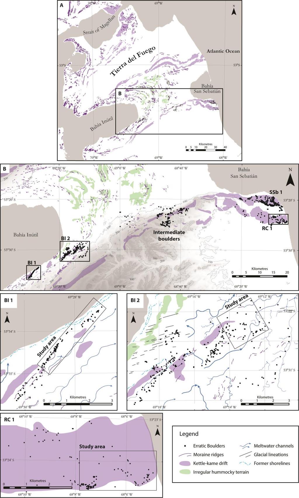
82 61

83 Figure 4.5. Previous 10 Be cosmogenic nuclide exposure dates from the boulder trains, as mean ages with standard errors (plotted in age order) and as probability plots; recalculated from the original data of McCulloch et al. (2005b), Kaplan et al. (2007), Kaplan et al. (2008a), and Evenson et al. (2009); and using the production rate of Putnam et al. (2010b) and the scaling model of Lal (1991) and Stone (2000). Note the substantial difference between the cosmogenic nuclide exposure dates and the hypothesised ages for RC 1 and SSb 1. 62

84 4.2.3 This study Kaplan et al. (2007) suggested that the occasional older dates for the EBTs on Tierra del Fuego were closer to the true age of the glacial limits and proposed that intense, episodic exhumation and/or erosion of the EBTs resulted in the samples yielding anomalously young ages (i.e., they are old boulders that were exhumed; Figure 4.6). However, an alternative hypothesis, not previously considered, is that all of the EBTs in Tierra del Fuego were deposited during the last glacial cycle (i.e., they are young boulders; Figure 4.6), and occasional samples are anomalously old owing to inheritance. The old hypothesis fits with the established age model but requires intense physical exhumation and erosion to explain the dates (Kaplan et al., 2007). The young hypothesis does not require such extreme processes, but questions the established age model and implies that ice was much more extensive during the last glacial cycle. This study tests between these two opposing hypotheses, and a summary of the expected weathering characteristics that might be found under these two different scenarios is given in Table

85 Figure 4.6. The different cosmogenic nuclide exposure dates from the RC 1 and SSb 1 boulders on Tierra del Fuego can be explained by two different hypotheses. (A) and (B) Illustrate the first hypothesis, proposed by Kaplan et al. (2007), which suggests that the majority of the boulders were exhumed and eroded subsequent to deposition, yielding anomalously young ages. (C) and (D) Illustrate the second hypothesis, proposed in this study, which suggests that occasional boulders may be anomalously old owing to inheritance because they were not sufficiently eroded by supraglacial transport. In this case, the majority of the cosmogenic nuclide exposure dates are a better representative of the age of the EBTs. 64

86 Table 4.2. Age and likely weathering characteristics for the Tierra del Fuego EBTs. Boulder train Properties BI 1 / BI 2 RC 1 if old a RC 1 if young b Hypothesised age 20 ka c ca. 450 ka c ka c Cosmogenic ages ca. 20 ka d ca ka e ca ka e Nature of erosion Likely agents of erosion Possible weathering rates Possibly some erosion Wind erosion, frost action, dissolution, mild salt-spray weathering Intense exhumation and erosion f Wind erosion, frost action, dissolution, salt-spray weathering Possibly some erosion Wind erosion, frost action, dissolution, salt-spray weathering mm ka -1 g > 25 mm ka -1 h mm ka -1 g Likely surface erosion 240 mm i > 11,250 mm j 360 mm k Likely erosional difference compared to BI 1 / BI 2 Roughness compared to BI 1 / BI 2 Hardness compared to BI 1 / BI 2 0 mm > 11,010 mm 120 mm N/A N/A Significantly rougher Significantly weaker Possibly slightly rougher or the same Possibly slightly weaker or the same a As hypothesised by Kaplan et al. (2007). b As hypothesised in this study. c Approximate ages, based on Meglioli (1992); Kaplan et al. (2007); Kaplan et al. (2008a). d McCulloch et al. (2005b); Kaplan et al. (2008a); Evenson et al. (2009). e Kaplan et al. (2007); Evenson et al. (2009). g Kaplan et al. (2005) calculated apparent erosion rates of roughly 0.5 to 2.5 mm ka -1 over > 760 ka for boulders deposited by the Lago Buenos Aires lobe in northern Patagonia. Kaplan et al. (2007) calculated apparent erosion rates of roughly 5 to 12 mm ka -1 over ca ka for boulders deposited by the Río Gallegos lobe in southern Patagonia. h Apparent erosion rate estimated by Kaplan et al. (2007). i j Assuming up to 12 mm ka -1 erosion over 20 ka. Assuming > 25 mm ka -1 erosion following rapid exhumation at 20 ka or continuous erosion at > 25 mm ka -1 over 450 ka. Kaplan et al. (2007) suggested that continuous erosion is unlikely given preservation of original surface geomorphology, so the amount of erosion is probably between these two end members. k Assuming up to 12 mm ka -1 erosion over up to 30 ka. 65

87 4.3 Methods Mapping and sampling We began by mapping all erratic boulders in the study area and then selected a sample of 150 boulders from three of the EBTs to compare trains hypothesised to be of similar and differing ages (Figure 4.3). Many of the boulders are sufficiently large and clear against the surrounding landscape for them to be mapped from remote imagery, so a map was produced to show their distribution using a combination of remote sensing analysis and field-checking. Aerial photographs from the Servicio Aerofotométrico de la Fuerza Aérea de Chile were used where possible as well as Google Earth imagery (version 7). Field-checking verified the broad spread of mapped boulders, and the locations of the 150 sampled boulders were recorded using a handheld Magellan explorist 610 GPS device. All boulders within a given area were sampled provided they were > 2 m in height. This was to avoid the effects of snow/vegetation cover and variable erosion on smaller boulders, and to avoid the chances of sampling fragments that may have broken off subsequent to deposition. Boulders were described in terms of basic lithology, surface appearance, and setting Size approximation, angularity, and appearance Boulders varied in size and accessibility, so boulder dimensions and volume were estimated using eight photographs taken around each boulder at roughly equal bearings. All photographs included a 1-m measuring-staff that was later used to gauge boulder height, width, and depth. The greatest measurement of height and width was used for each boulder as well as the corresponding largest depth measurement (perpendicular to greatest width). Volume was then calculated in three ways to give approximate upper, middle, and lower values, respectively: Cubic volume, calculated as: cubic volume = H W D Maximum inscribed cubic volume in a sphere, calculated as: Octahedral volume, calculated as: max. inscr. volume = ( ) H 2 W 2 D 2 3 octahedral volume = (H W D) Where H is boulder height, W is boulder width and D is boulder depth (Figure 4.7). 66

88 Figure 4.7. Visualisation of the three methods used to calculate boulder volume from the same measurements of Height (H), Width (W) and Depth (D). Volumes are approximations given the use of photographic analysis and that boulders are not regular shapes. Given the use of photographic analysis, measurements are given to the nearest 1 m. Volumes are still approximations given that boulders are not regular hexahedrons or spheres, but the cubic and octahedral volumes do provide likely maximum and minimum values from the field measurements. For boulders resting on the surface, volumetric values are likely to be correct, but many appear to be at least partially embedded, so that their height, and possibly width and depth, may be greater than was recorded. For the reasons given above, we suggest that our boulder volumes and boulder train volumes are only minimum estimates. Table 4.3. Criteria used to visually assess boulder roundness (Benn, 2004). Abbreviation Class Description VA Very Angular Edges and faces unworn; sharp, delicate protuberances A Angular Edges and faces unworn SA Sub Angular Faces unworn, edges worn SR Sub Rounded Edges and faces worn but clearly distinguishable R Rounded Edges and faces worn and barely distinguishable WR Well Rounded No edges or faces distinguishable 67

89 We measured angularity in two ways. Firstly, we assessed the roundness of each boulder according to a visual scale (Table 4.3). From this, we could calculate RA values (the percentage of angular and very angular boulders) as a measure of angularity (Benn & Ballantyne, 1994). We did not create corresponding C 40 values for the boulders because these would be biased by partial burial of some of the boulders. Secondly, we recorded the angularity of the most angular edge for each boulder in two of the boulder trains (BI 1 and RC 1; Figure 4.8). For this, we used an adapted version of the method of Kirkbride (2005). We used this technique in a simplistic way to compare relative differences in angularity between the boulder trains and did not manipulate the data beyond plotting the edge length against edge angle. Essentially, more angular edges create longer lengths and larger angles, and less angular edges create shorter lengths and smaller angles. The surficial characteristics and lithology of the boulders were also noted. Figure 4.8. Photograph and illustration of the technique used to measure angularity of boulder edges. The tool is similar to Kirkbride (2005) and measures the length and angle between two hinged points. Relative differences between the combinations of these values for different boulders relate to changes in edge angularity. 68

90 4.3.3 Schmidt hammer The Schmidt hammer has been used to measure rock-surface hardness as an indicator of the amount of time that rock has been exposed to subaerial processes (Matthews & Owen, 2010). Rebound values (R-values) produced by the impact of the hammer decline with increased rock-surface weathering, and can be used as a relative measure of exposure history (McCarroll, 1991; McCarroll & Nesje, 1993; Nesje et al., 1994; Goudie, 2006; Shakesby et al., 2011). We used an N-type Schmidt hammer to analyse 50 boulders from two of the boulder trains thought to be from different glacial cycles (BI 1 and RC 1). Fifty Schmidt hammer blows were recorded per boulder, with a total of 2500 blows per boulder train (5000 blows in total). On each boulder, 10 blows were recorded per face (approximately: north, east, south, west, and top) to explore whether aspect is a control on rock-surface weathering. The Schmidt hammer R-values were corrected for the angle at which the Schmidt hammer was held following Day & Goudie (1977), see Table 4.4. A correction was also made to account for instrumental drift based on an average trend, cross-checked against measurements on a calibration anvil. There are a number of potential limitations in using the Schmidt hammer as a relative dating tool. Small rock sizes and changes in lithology can influence results, although the boulders here were far larger than the minimum size suggested by Sumner & Nel (2002) and they were monolithological, and so this was not a limitation. Measurements can also be affected by discontinuities and moisture (especially in weak rocks), cracks, edges, and the surface roughness of the measured face (Goudie, 2006). Measurements were consistently taken on planar surfaces, away from cracks and edges, and our roughness measurements suggested little difference between the boulder trains. However, it is possible that the range of our results was caused by variability in these factors. Evans et al. (1999) also suggested that re-worked material may play a role in producing scattered R-values, although we suggest that this is unlikely to have been an issue given that the large size, high angularity and lack of subglacial abrasion of the boulders. 69

91 Table 4.4. Angle corrections applied to Schmidt hammer R-values (Day & Goudie, 1977). Correction for inclination angle Rebound value Upward impact Downward impact R Profile gauge Rock surface roughness can be used to compare the effects of weathering where it is assumed that initial surface texture was roughly the same (McCarroll & Nesje, 1993; 1996). This can then be used as an indicator of the relative time that a rock surface has been exposed to weathering processes. A profile gauge is a quick and easy tool for measuring rock surface roughness (McCarroll & Nesje, 1996), and we used a 25-cm gauge consisting of mm independent pins to sample planar rock surfaces. The profile gauge samples only a small part of any surface and cannot characterise the overall roughness of a boulder, but with numerous samples on numerous boulders, it can demonstrate relative differences in roughness between populations (McCarroll & Nesje, 1996). Converting the profiles into numerical values of roughness is the principal source of uncertainty. This has been discussed in detail in the literature (McCarroll & Nesje, 1996) and can be accounted for, to some degree, by comparing roughness wavelengths (8, 16, 24 and 32 mm in this case; Figure 4.9) and statistical techniques (Index A and RMS in this case). In this study, we assume that the glacial erosion and transport of all of the EBTs is essentially the same and that, given that the boulders are monolithological, differences in roughness result from the time exposed to weathering or variable weathering processes. The gauge was pressed firmly against the surface and then traced onto graph paper in the field and later digitized (Figure 4.9). Pin positions were recorded every 8, 16, 24 and 32 mm to evaluate different roughness wavelengths. We measured roughness profiles for 50 boulders in three boulder trains (BI 1, BI 2, and RC 2). Five profiles were recorded per boulder, making a total of 250 profiles per boulder train (750 profiles in total). On each boulder, one profile was recorded per face 70

92 (approximately: north, east, south, west, and top) to show whether roughness varied with aspect. Figure 4.9. The profile gauge used to measure rock surface roughness. Increasing the distance between measured points along the profile (i.e., the wavelength) has a smoothing effect, but also captures roughness at different resolutions. In this study, >20 mm wavelengths were the most useful. (A-D) illustrate the effects of surface slope on the recorded roughness. Hence, standard deviation removes the issue of surface curvature (adapted from McCarroll & Nesje, 1996). 4.4 Results Distribution We mapped a total of 1248 boulders and distinguished four EBTs. From innermost (ice-proximal) to outermost (ice-distal), these are: BI 1, BI 2, SSb 1, and RC 1 (Figure 4.4). In addition, a large spread of boulders lies between Bahía Inútil and Bahía San Sebastián (intermediates in Figure 4.4B). These are dispersed rather than tightly clustered and so are not classed as an EBT for the purposes of our study. However, we highlight that these intermediate boulders bridge the gap between BI 1 / BI 2 and SSb 1 / RC 1. It was not possible to access the SSb 1 EBT or some of the intermediate boulders for field-checking or analysis, but both were sampled for cosmogenic nuclide exposure dating by Kaplan et al. (2007). A summary of the characteristics of the boulder trains is given in Table 4.5 and example photos are given in Figures 4.10, 4.11 and

93 72 Table 4.5. The spatial characteristics and geomorphological context of the EBTs on Tierra del Fuego. Hypothesised ages are from Meglioli (1992). EBT No. boulders mapped Approx. train length (km) Approx. train width (km) Approx. train height (m asl) Spatial distribution Geomorphological context Hypothesised ages BI A highly linear train extending to the coast of Bahía Inútil. On a moraine belt, parallel to meltwater channels and with one meltwater channel dissecting it. MIS 2 BI Elements of linearity, but spread over a wider area than BI 1. May consist of more than one EBT, but not possible to distinguish in the field. Deposited across numerous moraines, with several meltwater channels cutting through. MIS 2 Intermediates Boulder density is much less than the other EBTs, so the boulders were not studied further. Lies across several moraines. Possibly relates to more than one glacial limit SSb Boulder density varies, delimited to the north and south by the extent of kettle and kame drift. Sits on a broad band of kettle and kame drift and continues eastward into the Atlantic Ocean. MIS 10 RC Boulder density varies, delimited to the north and south by the extent of kettle and kame drift. There are two tight, linear clusters of boulders roughly 1.7 km long and 1.5 km long. Sits on a broad band of kettle and kame drift and continues eastward into the Atlantic Ocean. MIS 12

94 Figure Example photographs of the BI 1 boulder train (A), surface texture (B) and boulders (C-H). A person and 1 m measuring staff is featured in A and C-H for scale. 73

95 Figure Example photographs of the BI 2 boulder train (A and B), boulders (C-F) and surface texture (G and H). A person and 1 m measuring staff is featured in C-F for scale. 74

96 Figure Example photographs of the RC 1 boulder train (A and B) and boulders (C-H). A person is featured in C-H for scale. 75

97 4.4.2 Volume characteristics The total volume of rock within the measured boulders in BI 1, BI 2, and RC 1 combined is > 22,000 m 3, within which the total volume of BI 1 is > 5,000 m 3, BI 2 is > 14,000 m 3, and RC 1 is > 2,000 m 3 (Figure 4.13). The largest boulders were in BI 2, with three boulders exceeding 1000 m 3. Of all boulders sampled, only one was found to be taller than it was wide, and we interpret this to indicate that almost all boulders are stable and at rest. Several examples of 4-6 near-consecutive boulders were found to increase in volume down-ice (Figure 4.13). This is masked in the field by scattered smaller boulders, and the pattern is least distinct in BI 2 where boulders are more dispersed. However, we suggest that these trends are real because they cannot be explained by measurement uncertainty or by changing the point from which EBT distance is measured Angularity Little difference in angularity was recorded between boulder trains, and all showed a dominance of angular or subangular boulders, supported by RA values of 64% for BI 1 / BI 2 and 54% for RC 1 (see Figure 4.14) Rock surface hardness The Schmidt hammer R-values were corrected for the angle at which the Schmidt hammer was held and for instrumental drift. The total mean R-values for the two boulder trains are 43.6 ±19.9 for BI 1 and 37.7 ±19.7 for RC 1 (Figure 4.15), and the means of different aspect faces also show consistently lower R-values for RC 1 than BI 1, in the range of A Mann-Whitney U test reveals a statistical difference between the median values of the two EBTs at the 0.95 significance level (p = < 0.05), when comparing total values and for each of the aspect faces. 76

98 Figure The results of boulder volume measurements. (A) Shows the results for all three boulder trains, which are shown individually beneath: (B) BI 1; (C) BI 2; (D) RC 1. Arrows highlight an apparent repeated pattern of increasing down-ice volume across several nearconsecutive boulders in all three EBTs. 77

99 Figure The results of angularity measurements. (A) Is a frequency histogram of observed boulder roundness, showing a dominance of angular boulders supported by high RA values (percentage of angular and very angular boulders). (B) Shows the similarity in boulder edge roundness between BI 1 and RC Rock surface roughness Following McCarroll & Nesje (1996), we present our roughness data in two ways. Index A uses the standard deviation of measurements and removes the influence of rock surface slope, whereas root mean square (RMS) represents roughness more accurately as the deviation from the mean, but will be affected by surface curvature (Figure 4.9). The profile gauge was used on all three boulder trains, and a strong correlation was found between Index A and RMS values (Figure 4.16), indicating that surface curvature did not affect the roughness results. Consequently, RMS values are used to assess differences in surface roughness (Figure 4.16). Reducing the wavelength reduces the mean roughness and spread of values, but McCarroll & Nesje (1996) suggested that lower wavelengths were unlikely to capture true 78

100 surface roughness. We found that the greatest rock crystal size was generally > 20 mm; hence we focus on the 32-mm wavelength data. The different number and spacing of data points along the profiles when the wavelength was varied did not affect the mean results, suggesting that the results indicate actual changes in roughness and are not caused by sampling strategy. The total mean values for the three boulder trains are 2.4 ±1.8 mm for BI 1, 2.3 ±1.6 mm for BI 2, and 2.8 ±2.3 mm for RC 1 at the 32-mm wavelength (Figure 4.16). Like the Schmidt hammer data, patterns exists within the roughness results, with RC 1 consistently showing greater roughness mean values mm greater than the lowest mean value from BI 1 or BI 2 for the total and different aspect faces. A Mann-Whitney U test shows a statistical difference between the total median values of all three EBTs at the 0.95 significance level (p = < 0.05). Likewise, some, but not all, of the aspect faces also show a statistical difference when comparing all three of the EBTs, and this applies when comparing BI 1 and BI 2 as well as BI 1 / BI 2 and RC 1.. Figure Results of Schmidt hammer rock hardness analysis on the BI 1 and RC 1 EBTs, as total data and split into directional faces. Mean data are shown with 2σ errors, in addition to frequency histograms that illustrate the overlap between the two boulder trains. 79

101 80 Figure Results of profile gauge rock surface roughness analysis on the BI 1, BI 2, and RC 1 EBTs, shown as frequency distributions. (A D) are Index A results and (E H) are RMS results. Note the similarity between the results of the two methods. RMS data is used in this study, focussing on the 32-mm wavelength.

102 4.5 Discussion Source Kaplan et al. (2007) and Evenson et al. (2009) described the boulders from BI 1, BI 2, and RC 1 as hornblende granodiorites. The only source for this lithology is a small area of the Cordillera Darwin mountain range (Figure 4.3), where lower Tertiary intrusive units outcrop within the former glacial accumulation area (Natland et al., 1974; Nelson, 1980; Evenson et al., 2009). This source suggests that the BI SSb ice lobe originated from the central Cordillera Darwin to the south. It also helps to position the ice divide between the BI SSb and Fagnano ice lobes at peak glaciation; and the presence of supraglacial rock debris on Tierra del Fuego implies that granodiorite nunataks existed within the central Cordillera Darwin during peak glaciation. Thus, peak ice thickness could not have exceeded around 2500 m, which acts as a constraint on ice cap reconstructions. The large boulders in Tierra del Fuego (up to 1000 m 3 ) are unlikely to have been transported subglacially given that erosion during the distance from their source (ca. 250 km) should have considerably reduced their size (Figure 4.2). Furthermore, our data show that the boulders are dominantly angular or subangular. Numerous angular boulders up to 21 m in diameter are unlikely to have been transported beneath the ice over such a long distance. We found no evidence of subglacial abrasion (e.g. polishing or striae), and the angularity of the boulders suggests that such signs have not been removed by weathering. A similar conclusion was reached by Evenson et al. (2009). As such, the most likely formation mechanism is supraglacial debris at the source location in the Cordillera Darwin. Previous workers all noted the tight distribution, large size, angularity, and monolithology of the EBTs on Tierra del Fuego (Meglioli, 1992; Bentley et al., 2005; McCulloch et al., 2005b; Evenson et al., 2009); and we suggest that these features match the characteristics expected of a supraglacial rock avalanche deposit (Shulmeister et al., 2009). Studies routinely estimate total rock avalanche deposit volumes of > 1,000,000 m 3 (Shugar & Clague, 2011; Sosio et al., 2012; Delaney & Evans, 2014) and even > 10,000,000 m 3 (Jibson et al., 2006; McColl & Davies, 2011; Shugar & Clague, 2011; Sosio et al., 2012), far in excess of our minimum estimates of > 22,000 m 3 (or > 150,000 m 3 assuming that the coarse fraction accounts for around 15% of the total volume; Delaney & Evans, 2014). This suggests that the size of the deposit is not unreasonable for a supraglacial rock avalanche. The clustering of the EBTs suggests that the erosion of the boulders 81

103 occurred in discrete events and implies that gradual erosion at the source is improbable. Debuttressing during glacial retreat could have resulted in episodic deposition of debris caused by joint failures. However, we note that the boulders cut across a range of glacial geomorphology both small moraine ridges and kettle and kame topography (Figure 4.4) and that the RC 1 EBT was deposited when the ice lobe was still fully extended. Additionally, whilst the EBTs might have been deposited during recession, they represent flowline features, not ice-marginal deposits. The production of boulder trains as a result of supraglacial rock avalanches has not been explicitly examined in previous work. Shulmeister et al. (2009) noted that for large supraglacial rock avalanches, a greater proportion of thicker debris remains on the glacier surface rather than being incorporated into the subglacial system, and a characteristic carapace of coarser debris generally caps deposits (Reznichenko et al., 2011). Coarse distal rims are found in numerous deposits (Hewitt, 1999; Chevalier et al., 2009; Hewitt, 2009; McColl & Davies, 2011; Shugar & Clague, 2011) and, theoretically, these could result in boulder trains, especially if divergent flowlines drew the boulders into a train prior to deposition (Evenson et al., 2009). However, large boulders may also be found across the debris sheet, with the rim simply representing a greater density of large boulders caused by bulldozing (Shugar & Clague, 2011). It thus remains unclear exactly how a rock avalanche debris sheet is transformed into EBTs, but we now discuss a conceptual model for their transport and deposition Transport and deposition The lateral position of the EBTs on Tierra del Fuego probably resulted from ice to the north (the Magellan lobe) deflecting the BI SSb lobe to the east (Figure 4.3), with divergent flow lines focusing the boulders in a lateral position (Evenson et al., 2009). Thus, we envisage that the boulders were transported supraglacially from the central Cordillera Darwin, east of Isla Dawson, before turning sharply east into Bahía Inútil to be deposited on the south side of the former ice lobe (Figure 4.3). Given that the Cordillera Darwin has experienced seismic activity in the past (Cunningham, 1993; Klepeis, 1994; Bentley & McCulloch, 2005), the four distinct boulder trains may have resulted from separate rock avalanche pulses (Larsen et al., 2005; Jibson et al., 2006). Ice crevassing, subaerial weathering, and meltwater may have acted to remove much of the finer material (Shulmeister et al., 2009), and 82

104 ice flow and the divergence of flow lines then dragged the distal rim and boulder carapace into trains (Evenson et al., 2009). Our mapping shows that the EBTs are significantly more extensive than previously thought (Evenson et al., 2009) and occur at several places along the southern limit of the former ice lobe. There are also numerous boulders that do not cluster as boulder trains (intermediates), but act as a continuum between BI 1 / BI 2 and SSb 1 / RC 1. Whilst the EBTs may represent distinct spatial and temporal events (as proposed by Kaplan et al., 2007, and Evenson et al., 2009), they could also represent rock avalanche pulses during the same period, possibly linked to seismic activity (Larsen et al., 2005; Chevalier et al., 2009). Studies in New Zealand have suggested that supraglacial rock avalanches may result in the deposition of nonclimatic moraines (Anderson & Mackintosh, 2006; Tovar et al., 2008; Shulmeister et al., 2009; Reznichenko et al., 2011). However, given the small area and isolated nature of the EBTs compared to the area covered by the BI SSb ice lobe, a similar debris-induced, non-climatic model is improbable. The patterns of increasing down-ice boulder volume observed within each of the EBTs (Figure 4.13) are unlikely to have been preserved in any scenario other than deposition onto and transport on top of the former ice. However, the formation of these patterns is unclear. Little evidence suggests that gravitational sorting of avalanche debris occurs (Marangunic & Bull, 1968; Shugar & Clague, 2011), but trains of debris several metres wide and parallel to the direction of debris flow have been described (Hewitt, 2009; Shugar & Clague, 2011; Delaney & Evans, 2014). These likely resulted from snow ploughing of a large boulder, with finer material following behind on exposed glacial ice (Delaney & Evans, 2014), and currently offer the best analogue for the patterns of boulder size trends seen in Tierra del Fuego Rock surface weathering The Schmidt hammer data show a statistical difference between the RC 1 and BI 1 EBTs, indicating that the RC 1 boulders have been subjected to a greater degree of weathering than the BI 1 boulders. However, the differences are not as great as might be expected if intense, episodic erosion has taken place (Table 4.2). The R- values showed a total average difference of 5.9, whereas McCarroll & Nesje (1993) demonstrated differences of between Little Ice Age and late glacial sites in western Norway; and Matthews & Owen (2010) highlighted differences of between Little Ice Age and Preboreal sites in southern Norway. Rock weathering (and therefore R-values) could have reached saturation in Tierra del Fuego. 83

105 However, despite agreement that R-values will progress toward a dynamic equilibrium over time (White et al., 1998; Engel, 2007; Sánchez et al., 2009; Černá & Engel, 2011; Stahl et al., 2013), numerous studies have effectively distinguished glgm and pre-glgm deposits using the technique on timescales of 10s to 100s ka (Ballantyne et al., 1997; Rae et al., 2004; Černá & Engel, 2011; Stahl et al., 2013). Very high rates of weathering are required to reduce the ages of the RC 1 boulders (Table 4.2), yet no obvious jump in R-values occurs between these and the BI 1 / BI 2 boulder trains. The roughness data show a statistical difference between the total values of RC 1 and BI 1 / BI 2, but also between the BI 1 and BI 2 total values. Because BI 1 and BI 2 are assumed to be roughly the same age (lying within the same ice marginal deposits; Figure 4.3), this implies that the difference between RC 1 and BI 1 / BI 2 is not necessarily related to a significant difference in age. Differences between BI 1 and BI 2 could be driven by the highly variable values measured for the top aspect faces of the boulders, but statistical similarities also exist between the BI 1 / BI 2 and RC 1 aspect faces, suggesting that any differences are unlikely to be the result of a large difference in age between these EBTs. Most importantly, and like the Schmidt hammer data, we do not find a jump in values between RC 1 and BI 1 / BI 2 that might be expected if intense, episodic erosion has taken place (Table 4.2). The average total difference in roughness between RC 1 and BI 2 is 0.5 mm at the 32- mm wavelength. Given that the large crystal size is > 20 mm and that the averages for all three boulder trains are between 2.3 and 2.8 mm, this difference is negligible. McCarroll & Nesje (1996) recorded much greater differences in roughness values when studying salt spray and chemical weathering of boulders. We cannot directly compare studies of different lithologies in different environments, but we would expect a clear difference in roughness values between the RC 1 and BI 1 / BI 2 boulder trains if intense erosion has occurred. Kaplan et al. (2007) suggested that proximity to the coastline may have caused higher rates of salt-spray weathering of the RC 1 boulders. Similarly, the dominant effect of the westerly winds in the region could have caused increased aeolian abrasion. Figure 4.17 shows the results for averaged rock surface hardness and rock surface roughness from each boulder, with total boulder values and east/west faces shown. Correlations between these results and the distance from the start of the BI 1 and RC 1 boulder trains are negligible. Given the variability in the data, there is no indication that salt-spray weathering or aeolian abrasion has had a 84

106 variable effect on boulders within RC 1 or a markedly greater effect on RC 1 than BI1. Weathering could have been operating on a scale greater than that recorded by our proxies. However, whilst examples of microgullies and potholes are abundant on the top surfaces of the RC 1 boulders (Kaplan et al., 2007), similar features exist on the BI 1 and BI 2 boulders, and we found little difference in top surface weathering between the boulder trains (Figures 4.10, 4.11 and 4.12). The similarity in weathering results between the EBTs suggests that they have probably experienced similar local climatic conditions. This is important given that the intense weathering needed to reduce the ages of the RC 1 boulder train during, or since, the glgm should have also reduced the ages of the BI 1 and BI 2 boulder trains. The cosmogenic exposure dates for the BI 1 and BI 2 boulder trains are believed to be good estimates of the time of deposition (around the glgm), agreeing with radiocarbon dates in the area (Heusser, 2003; McCulloch et al., 2005b; Kaplan et al., 2008a; Hall et al., 2013) and factors that reduced the RC 1 boulder dates by hundreds of thousands of years are highly unlikely to have also reduced the BI 1 and BI 2 dates. 85

107 Figure The rock surface hardness and roughness results from Figures 4.15 and 4.16 plotted to illustrate variations in aspect with distance along the boulder trains (data points relate to individual boulders and are only shown for BI 1 and RC 1). (A) Shows hardness results for the east and west faces of BI 1, and (B) shows roughness results for the east and west faces of BI 1. (C) Shows hardness results for the east and west faces of RC 1, and (D) shows roughness results for the east and west faces of RC 1. In all graphs, boulder values toward the right are located farther to the east and those toward the left are located farther to the west. No discernible trends are found in either of the boulder trains, as illustrated by very low R 2 values, suggesting that salt weathering has not affected RC 1 significantly more than BI 1, as hypothesised by Kaplan et al. (2007), despite closer proximity to the coast. 86

108 4.5.4 Alternative (post-)depositional model The EBTs on Tierra del Fuego were thought to have been deposited during different glacial episodes (MIS 12, 10, and 2), but cosmogenic nuclide exposure dating from all of the EBTs yielded dates predominantly around 20 ka (Kaplan et al., 2007; Evenson et al., 2009). One hypothesis (the boulders are old ) explains this anomaly by invoking intensive post-depositional exhumation and erosion of the RC 1 boulders (Kaplan et al., 2007), but a second (the boulders are young ) suggests that supraglacial debris may have an inheritance signature. Our study demonstrates that the distribution, volume, and monolithology of the boulder trains are indicative of supraglacial transport of rock avalanche material, and our rock surface weathering data do not support intensive post-depositional exhumation and erosion of the RC 1 boulders. Given this information, our data support the second, young hypothesis, whereby the EBTs were transported and deposited at roughly the same time (i.e. within a few thousands of years, rather than separated by 100s of thousands of years). Under this scenario, one would anticipate mostly young ages from the boulders, but with some anomalously old dates resulting from an inheritance signal owing to pre-exposure of boulders in the cliff face, which were not then sufficiently eroded during supraglacial transport (Applegate et al., 2010; Heyman et al., 2011; Applegate et al., 2012). This scenario is similar to that envisaged for the Foothills boulder train in Alberta, where Jackson et al. (1997) suggested that an erratic boulder that yielded a date of ca. 53 ka (four times older than the next oldest date) was improbable and most likely caused by pre-exposure prior to glacial transport. This implies that, for a supraglacial EBT deposit, a fraction of boulders should be expected to yield anomalously old dates. Assuming that the majority of 10 Be cosmogenic exposure dates are roughly correct, three anomalously old dates are apparent from the Tierra del Fuego boulder trains (Kaplan et al., 2007; Evenson et al., 2009). For RC 1, one date (ca. 57 ka) out of 7; and for BI 2, one date (ca. 56 ka) out of 17 may have been pre-exposed. The similarity between these ages could indicate a consistent (pre-) exposure pattern, but more samples would be needed to support this idea. The outlier from SSb 1 is significantly older at ca. 222 ka, although this is only one of two samples from that boulder train. Leaving aside the anomalously old dates, substantial variability remains in the cosmogenic nuclide exposure dates of the RC 1 EBT, a fact that Kaplan et al. (2007) highlighted. Variability in the dates could have been caused by variability in 87

109 the residence time on the ice during transport. Hubbard et al. (2005) modelled ice flow velocities of up to 2000 m a -1 for the northern Patagonian Ice Sheet. Assuming similar velocities and a transport distance of up to 250 km for the BI SSb lobe, transport time may have been as little as ka: insignificant given dating uncertainty. Slower velocities of 100 m a -1 or even 50 m a -1 would have resulted in residence times of 2.5 or 5 ka, respectively; but given that the clustering of the EBTs suggests that they were deposited as discrete events, this could only have resulted in age differences between, not within, boulder trains. Rather, we suggest three mechanisms that could have produced the variability in RC 1. First, RC 1 has probably experienced greater erosion than BI 1 / BI 2 as it was deposited first, causing variable reduction in cosmogenic nuclide exposure dates. Secondly, we agree with Kaplan et al. (2007) that many boulders in the RC 1 train show signs of surface weathering, although we find similar signs in the BI 1 / BI 2 EBTs. Sampling of the RC 1 boulder train may have been more affected by weathered surfaces than BI 1 / BI 2 because fewer larger boulders are found in RC 1 and this could have resulted in sampling of boulders that were less ideal than those in the other boulder trains. Thirdly, Jackson et al. (1997) suggested that boulder orientation can affect the spread of dates in a boulder train. We have demonstrated that all boulders in Tierra del Fuego are likely at rest, but do not know how long they were sitting on melting ice before reaching this state. The RC 1 and SSb 1 boulder trains are located on large bands of kettle kame drift, a characteristic deposit of dead ice terrain (Dyke & Evans, 2003; Schomacker, 2008), whereas BI 1 and BI 2 are located on small, sharp moraines interspersed by meltwater channels. Ground ice within the kettle and kame topography could have taken a long time to fully melt and settle, and occasional examples of boulders exposed at the coastline, within the kettle and kame deposits, may be a result of this slow process of settling (Figure 4.12H). Thus, the RC 1 boulder train may have taken ca. 10 ka to come to rest and implies that ground ice melting may have prevailed long after the recession of the ice lobe. To summarise, the main implication behind this alternative history of the EBTs on Tierra del Fuego is that the established age model for the timing of glaciations in the region may need re-examining. Whilst this study provides a new approach to interpreting the cosmogenic nuclide exposure dates, further independent age controls for the glacial limits are needed to investigate the timing of glacial advances. 88

110 4.6 Conclusion Erratic boulder trains make valuable targets for flow-line indicators and cosmogenic nuclide exposure dating, but few have been reported in detail and further studies are needed to understand their formation, transport, and deposition. Based on the limited number of EBTs that have been reported in the literature, we identify an apparent trend between boulder size, transport distance, and likely mode of transport. The EBTs containing boulders greater than ca. 5 m in diameter and/or demonstrating transport from the source lithology of greater than ca. 10 km are likely to have been transported supraglacially. In Tierra del Fuego, the distribution and volume of three boulder trains suggest that they were formed by a rock avalanche and transported and deposited supraglacially. This highlights a former ice flow line from the Cordillera Darwin and helps to constrain the position of ice divides and the maximum ice surface elevation. Using a variety of techniques and measurements, we do not identify any major changes in rock surface weathering characteristics across EBTs that have been previously interpreted to be from different glacial cycles. Thus, we suggest that they are much closer in age (probably within a few thousand years), which is also consistent with previous cosmogenic nuclide exposure dates from the boulders. Occasional, anomalously old samples should be expected from supraglacial boulder trains caused by pre-exposure prior to and during glacial transport, and an understanding of the likely history of an EBT should be an integral part of using the features for dating. 89

111 Chapter 5. Extensive MIS 3 glaciation in southernmost Patagonia revealed by cosmogenic nuclide dating of outwash sediments Darvill, C.M., Bentley, M.J., Stokes, C.R., Hein, A.S. & Ródes, Á. (in prep.) Extensive MIS 3 glaciation in southernmost Patagonia revealed by cosmogenic nuclide dating of outwash sediments, Earth and Planetary Science Letters. 90

112 Abstract The timing and extent of former glacial advances can demonstrate leads and lags during periods of climatic change and their forcing, but this requires robust glacial chronologies. In southernmost Patagonia, dating pre-glgm ice limits has proven difficult due to post-deposition processes affecting the build-up of cosmogenic nuclides in moraine boulders. Here we provide ages for the Río Cullen and San Sebastián glacial limits of the former BI-SSb ice lobe on Tierra del Fuego (53-54 S), previously hypothesised to represent advances during MIS 12 and 10, respectively. Our approach uses cosmogenic 10 Be and 26 Al exposure dating, but targets glacial outwash associated with the limits and uses depth-profiles and surface cobble samples, thereby accounting for surface deflation and inheritance. The data reveal that the limits formed more recently than previously thought, giving ages of 45.6 ka (+139.9/-14.3) for the Río Cullen, and 30.1 ka (+45.6/-23.1) for the San Sebastián limits. These dates indicate extensive glaciation in southern Patagonia during MIS 3, prior to the well-constrained, but much less extensive MIS 2 glgm limit. This suggests the pattern of ice advances in the region was different to northern Patagonia, with nested limits relating to the last glacial cycle, rather than progressively less extensive glaciations over hundreds of thousands of years. However, the dates are consistent with MIS 3 glaciation elsewhere in the southern mid-latitudes, and the combination of cooler summers and warmer winters, with increased precipitation, may have caused extensive glaciation prior to the glgm. 91

113 5.1 Introduction The terrestrial record of former Southern Hemisphere ice masses has been used to assess inter-hemispheric synchroneity of glacial advance and retreat (Sugden et al., 2005; Kaplan et al., 2010; Putnam et al., 2013a) and how climatic forcing, such as changes in the Southern Westerly Winds (Figure 5.1), triggered ice growth or wastage through time (Kohfeld et al., 2013). Patagonia is an ideal location for such records given that it spans a large latitudinal range and exhibits well-preserved glacial geomorphology reflecting former advances of the Patagonian Ice Sheet. However, coupling glacial reconstructions with robust chronologies is challenging. Figure 5.1. (A) Location of the study area, with shading indicating the approximate present extent of the Southern Westerly Wind system. (B) Map of Patagonia with glgm ice extent from Singer et al. (2004a). (C) Drift limits of the former BI-SSb ice lobe across northern Tierra del Fuego from Meglioli (1992) and Chapter 3. Dashed lines indicate inferred extents. Stars show approximate locations of previously published 10 Be exposure dates from boulder trains (McCulloch et al., 2005b; Kaplan et al., 2007; Evenson et al., 2009), and the Filaret and Cullen depth profiles from this study are labelled. The Bahía Inútil drift (4) correlates with the glgm. (D) Previously published 10 Be dates, shown as cumulative probability density function plots (McCulloch et al., 2005b; Kaplan et al., 2007; Evenson et al., 2009). Graphs are labelled according to drift limits in C, along with the published hypothesised MIS age (Coronato et al., 2004) and the number of samples. One additional exposure date for limit 2 is 222 ± 7 ka. 92

114 The established model for the timing of glaciations in this region hypothesises that, following the 1.1 Ma GPG (Caldenius, 1932), the Patagonian Ice Sheet lobes oscillated in unison, creating a pattern of nested glacial limits resulting from a series of progressively less-extensive glaciations throughout the Quaternary (Coronato et al., 2004; Figure 5.1). Chronologies from northern Patagonia have demonstrated such a pattern (Singer et al., 2004a; Kaplan et al., 2005; Hein et al., 2009; Hein et al., 2011), but the timing of glacial advances in southernmost Patagonia is more open to conjecture. On Tierra del Fuego, moraines hypothesised to have been deposited during MIS 12 (ca. 450 ka) and MIS 10 (ca. 350 ka) have been dated using cosmogenic nuclide exposure dating of erratic boulders and yielded dates centred around ca. 21 ka, similar to the glgm limit (Figure 5.1; Kaplan et al., 2007; Evenson et al., 2009). It has been suggested that this could be due to intense post-depositional exhumation and erosion of the boulders from MIS 12/10 limits (Kaplan et al., 2007), but an alternative hypothesis, suggested here, is that the dates are closer to the true age of the glacial advance whereby, following the GPG, the ice lobe was most extensive during the last glacial cycle (MIS 4-2). In this study, we test these two opposing hypotheses using a new method that can account for post-depositional exhumation processes. Specifically, Hein et al. (2009) demonstrated that cosmogenic nuclide depth-profiles through outwash associated with moraine limits can yield robust ages for glacial limits where post-depositional erosion and exhumation may compromise traditional moraine-boulder samples. We present 10 Be and 26 Al dates from two depth profiles through outwash associated with glacial limits of the BI-SSb ice lobe on Tierra del Fuego (53-54 S) and use these results to test the established age model for the timing of glacial advance. 5.2 Study area The BI-SSb depression in central Tierra del Fuego was the former location of an eastward flowing ice-lobe sourced from the Cordillera Darwin range to the southwest (Evenson et al., 2009; and Chapter 4). Two large bands of kettle and kame drift (Figures 5.2 and 5.3) correspond with two former ice limits (Figure 5.1). The inner limit is the San Sebastián drift (Meglioli, 1992) and is hypothesised to date from MIS 10 based on correlations to Uranium-series dated marine terraces (Bujalesky et al., 2001; Coronato et al., 2004). The outer limit forms the Río Cullen drift (Meglioli, 1992), and is hypothesised to date from MIS 12 (Coronato et al., 2004) based on ages of <760 ka by palaeomagnetism of basal till (Walther et al., 2007). However, direct cosmogenic nuclide exposure dating of boulders on both drifts yielded 93

115 substantially younger ages, ranging from 15 to 222 ka with most <50 ka (Figure 5.1; Kaplan et al., 2007; Evenson et al., 2009). 5.3 Methods Sampling We identified locations where the San Sebastián and Río Cullen limits could be linked unequivocally to their associated outwash units. An overview of the glacial geomorphology of this part of Tierra del Fuego is shown in Figure 5.2, and an enlarged version of the sampling area is shown in Figure 5.3 (see also Appendix). The outwash is considered to relate unambiguously to the glacial limits in question and, in both cases, it was possible to walk directly from the sample locations on the outwash surfaces onto the kettle kame drift deposits of the glacial limits. The outwash surfaces retained original surface morphology and appeared to be relatively undisturbed. The path of meltwater issuing from the inner San Sebastián glacial limit could be clearly traced through the outer Río Cullen glacial limit, and formed an incised channel in the Río Cullen outwash surface that did not affect the Cullen profile (Figure 5.4). Furthermore, meltwater younger than the San Sebastián glacial limit was topographically confined to the central BI-SSb depression (Figure 5.4), where it flowed directly east toward the Atlantic. Two depth profiles were sampled at these locations, relating to the San Sebastián glacial limit (Filaret profile) and the Río Cullen glacial limit (Cullen profile; Figure 5.1). The surfaces of these units possessed a well preserved morphology (e.g. braided meltwater channels), graded directly to the moraines of the drift limit (Figures 5.6 and 5.9), and showed no evidence of post-depositional reworking. Consequently, they are ideal locations for dating using outwash depth-profiles (Hein et al., 2009; Hein et al., 2011). 94

116 95 Figure 5.2. The glacial geomorphology of the former BI-SSb ice lobe in Tierra del Fuego, adapted from Chapter 3.

117 96 Figure 5.3. Zoomed version of Figure 5.2 to show the sampling area and the locations of the depth profiles, adapted from Chapter 3.

118 Figure 5.4. Transects A-A and B-B from Figure 5.3 showing the elevation change across the glacial drift limits and the sampled outwash. 97

119 The depth profiles were sampled from exposures within small, contemporary roadside quarries. These were cleared and logged, exhibiting sediments ranging from silts to cobbles of various, mixed lithologies (Figures 5.6 and 5.9). Our field observations suggested that each outwash terrace accumulated continuously as a discrete deposit associated with the meltwater issuing from the nearby glacial limit. Both were covered in low grass and were capped by brown, silty, poorly-developed soils up to ~ 25 cm deep. Each contained a single outwash unit of silts, sands, gravels and cobbles at various grades, but with no obvious signs that their source had changed over time. There were no frost wedges within the sediments and no clear signs of cryoturbation or pedogenic carbonate formation. Depths through the outwash were measured with a tape measure from the surface and were demarcated for sampling using a spirit level and spray-paint. We followed Hein et al. (2009) in collecting depth and surface samples to allow modelling of cosmogenic 10 Be and 26 Al accumulation to give a most probable unit age, whilst constraining inheritance and post-depositional surface erosion. Small (ca. 6 cm) quartz cobbles embedded within the outwash surface in the vicinity of the exposures were sampled, crushed whole, and analysed individually as independent estimates of exposure time shown before and after sampling in Figures 5.7 and We also collected ~1 kg samples of mixed lithology pebbles (>0.5 cm and <4 cm) at 25 cm depth intervals (depth error 4 cm), including a sample at the base of the section to help calculate inheritance in the profile. Each depth sample was amalgamated and analysed for 10 Be and 26 Al concentrations. One sample (FP025cs) consisted half of sand matrix due to insufficient clasts at that depth. In both profiles the lowermost sample consisted of two separate depth samples combined (i.e. an unprocessed weight of ~ 2 kg) due to insufficient quartz; hence the apparent thickness of these samples is greater. All physical and chemical preparation and 10 Be/ 9 Be and 26 Al/ 27 Al AMS measurements were carried out at the Scottish Universities Environmental Research Centre (SUERC) as part of the NERC Cosmogenic Isotope Analysis Facility (CIAF), as per Wilson et al. (2008). 98

120 99 Figure 5.5. Panorama of the Filaret profile location (top) with annotations (bottom). (W)est, (N)orth and (E)ast directions are shown.

121 Figure 5.6. (A) Photograph of the Filaret depth profile during sampling. The top of the profile was taken from the local soil level, given there was also some spoil from the quarry. (B) sediment log and description for the Filaret profile, highlighting the depths of samples analysed in this study. 100

122 Figure 5.7. Pictures of the surface cobble samples from the Filaret profile before (left) and after sampling (right). Each caption shows the sample name, and those on the right also show the calculated 10 Be / 26 Al ages from Table

123 102 Figure 5.8. Panorama of the Cullen profile location (top) with annotations (bottom). (E)ast, (S)outh and (W)est directions are shown.

124 Figure 5.9. (A) Photograph of the Cullen depth profile during sampling. The top of the profile was taken from the local soil level, given there was also some spoil from the quarry. (B) sediment log and description for the Cullen profile, highlighting the depths of samples analysed in this study. 103

125 Figure Pictures of the surface cobble samples from the Cullen profile before (left) and after sampling (right). Each caption shows the sample name, and those on the right also show the calculated 10 Be / 26 Al ages from Table

126 5.3.2 Chemical analysis Surface cobbles were treated individually, whereas depth samples were treated as amalgams. All samples were crushed whole, milled and sieved, and the >125 μm <500 μm fraction was then magnetically separated using a Frantz machine prior to chemical analysis. They were treated with a 2:1 mixture of H 2 SiF 6 and HCl on a shaker table to dissolve non quartz minerals. The quartz was then purified by repeat etching in HF on a shaker table to remove >30 % of the starting mass; with the ion concentration gauged using assays measured by ICP-OES. All samples were dissolved in 40% HF dry-downs on a hotplate. 0.2 mg of 9 Be carrier was added to each sample and 26 Al carrier was added to most samples so that 2 mg of Al per sample was reached. The solutions were passed through anion exchange columns to remove Fe and other contaminants, and then precipitated to remove Ti prior to being passed through cation exchange columns to separate Be and Al. The separate Be and Al fractions were precipitated and converted to BeO and Al 2 O 3, before being prepared for AMS analysis. NIST-SRM4325 and PRIME-Z primary standards were used for AMS measurements, with nominal ratios of Be/ 9 Be and Al/ 27 Al, respectively. The reported uncertainties of the nuclide concentrations include 2.5% for the AMS and chemical preparation. Blank corrections ranged between 3 and 15% of the sample 10 Be/ 9 Be ratios and between 0 and 0.9% of the sample 26 Al/ 27 Al ratios. The uncertainty of the blank measurements is included in the stated uncertainties. 105

127 106 Table 5.1. Sample descriptions and nuclide concentrations. Latitude Longitude Altitude Elv. Thickness Density Shielding Erosion Be ID Al ID Type * Sample ID (DD) (DD) (m asl) flag (cm) (g cm -2 ) correction (cm yr -1 ) Filaret profile 10 Be 1σ Be AMS (atoms g -1 ) (atoms g -1 ) std 26 Al 1σ Al AMS b6888 a1765 a FP025CS std NIST_ Z b6889 a1766 a FP std NIST_ Z b6890 a1767 a FP std NIST_ Z b6891 a1768 a FP std NIST_ Z b6892 a1769 a FP std NIST_ Z b6894 a1771 a FP std NIST_ Z b6895 a1772 s FPSS std NIST_ Z b6896 a1773 s FPSS std NIST_ Z b6897 a1774 s FPSS std NIST_ Z b6898 a1775 s FPSS std NIST_ Z Cullen profile b6903 a1778 a CP std NIST_ Z b6904 a1819 a CP std NIST_ Z b6905 a1779 a CP std NIST_ Z b6906 a1780 a CP std NIST_ Z b6908 a1820 a CP std NIST_ Z b6909 a1821 a CP std NIST_ Z b6910 a1781 s CPSS std NIST_ Z b6911 a1782 s CPSS std NIST_ Z b6912 a1784 s CPSS std NIST_ Z b7197 a1785 s CPSS std NIST_ Z * a amalgamated depth profile sample; s individual surface cobble sample. depth sample thickness set at a standard 4cm error, with amalgamated samples including the depth between samples; surface cobble samples set at a standard 6cm error. surface sample density is estimated at 2.7 g cm -3 ; depth samples density is constrained during modelling. (atoms g -1 ) (atoms g -1 ) std

128 107 Table 5.2. Calculated ages for surface samples using CRONUS-Earth calculator (Balco et al., 2008). Grey shading indicates the production rate and scaling scheme used. Sample ID Filaret profile Be P NZ P PTGN P GLOBAL P NZ St De Du Li Lm Lm Lm Lm age (a) ± age (a) ± age (a) ± age (a) ± age (a) ± age (a) ± age (a) ± age (a) ± FPSS FPSS FPSS FPSS Al FPSS FPSS FPSS FPSS Cullen profile Be CPSS CPSS CPSS CPSS Al CPSS CPSS CPSS CPSS Production rates: P NZ New Zealand production rate of Putnam et al. (2010b); P PTGN Patagonian production rate of Kaplan et al. (2011); P GLOBAL global production rate of Balco et al. (2008) and Nishiizumi et al. (2007). Scaling schemes: St Lal (1991) and Stone (2000); De Desilets et al. (2006); Du Dunai (2001); Li Lifton et al. (2005); Lm time-dependent version of Lal (1991) and Stone (2000).

129 5.3.3 Age determination Scaling scheme and production rate For consistency, the time-dependent scaling scheme of Lal (1991) and Stone (2000) was used in surface sample age calibrations and recalibrations of published data. Likewise, the production rate of Putnam et al. (2010b) from New Zealand was used throughout to calibrate 10 Be and 26 Al measurements, given that it is now in common use in Patagonia and the Southern Hemisphere and that it overlaps at 1σ with an independent production rate from Lago Argentino in Patagonia (Kaplan et al., 2011; see Table 5.2). We assessed the implications of choosing this production rate and scaling scheme combination using our surface sample ages calculated using the New Zealand production rate and Lal (1991) and Stone (2000) time-dependent scaling scheme. The global production rate gave ages <17% older or younger than our ages (irrespective of scaling scheme), but the Patagonian production rate gave ages <6% older or younger than our ages (irrespective of scaling scheme) or <5% older or younger when the same scaling schemes were compared. Using the New Zealand production rate, altering the scaling scheme resulted in <3% older or younger ages. Therefore, aside from not using the global production rate, our choice of production rate and scaling scheme does not alter our conclusions. Table 5.3. Details of comparison moraine boulder 10 Be chronologies from Patagonia for the last 100 ka. Where appropriate, updated data from Kaplan et al. (2011) have been used. Ice lobe Total no. 10 Be dates References Lago Buenos Aires 77 Douglass et al. (2005); Kaplan et al. (2004); Kaplan et al. (2005); Douglass et al. (2006) Lago Pueyrredón 12 Hein et al. (2009); Hein et al. (2011) San Martín valley 10 Glasser et al. (2011) Última Esperanza (Bella Vista / Río Gallegos lobe) 8 Sagredo et al. (2011); Kaplan et al. (2007); Evenson et al. (2009) Magellan 17 Bahía Inútil San Sebastián 41 McCulloch et al. (2005b); Kaplan et al. (2007); Kaplan et al. (2008a) McCulloch et al. (2005b); Kaplan et al. (2007); Kaplan et al. (2008a); Evenson et al. (2009) 108

130 Surface samples Apparent 10 Be and 26 Al exposure ages and internal uncertainties from surface sample measurements were calculated using the CRONUS-earth online calculator version 2.2 (available at Wrapper script: 2.2; Main calculator: 2.1; Objective function: 2; Constants: 2.2.1; Muons: 1.1; see Balco et al., 2008). We assumed a density of 2.7 g cm -3 (equivalent to the density of pure quartz) and used a standard, excess thickness of 6 cm for all samples to correct for self-shielding. Topographic shielding was measured in the field using an abney level but this correction was minimal (scaling factor > ). Present day snow and vegetation cover is thin, and is unlikely to have increased during glacial times, so no correction was applied for shielding by snow cover or vegetation. Likewise, no erosion correction was applied given that the quartz cobbles showed no significant signs of surface erosion. As a result of these assumptions, the ages should be considered minimum estimates Depth profiles The depth profiles were modelled using Hidy et al. (2010; version 1.2), which applies Monte Carlo simulations to find the most probable values for surface exposure age, erosion rate and nuclide inheritance. For both depth profiles, there were samples that deviated from the theoretical nuclide decay curve: FP150 for the Filaret profile and CP75 and CP150 for the Cullen profile. We tested whether these were outliers by running the model with wide parameters, initially including all samples (the model would not run) and then excluding all the samples one at a time. The model would only run with the outliers mentioned above removed from the profiles and they were not included in further modelling. This resulted in normally decreasing nuclide concentrations with depth, though the modelling was constrained by fewer samples. The 26 Al/ 10 Be ratio for CP150 plotted well below the steady state erosion island (Figure 5.11), normally indicative of a period of burial that results in a lower 26 Al/ 10 Be ratio. However, it is unclear why the FP150 and CP75 samples yielded anomalous results, given that the 26 Al/ 10 Be ratios are not low. Furthermore, there is no evidence for changing sedimentary processes at any of these three depths. Alternatively, anomalous results could have been caused by issues with the physical or chemical preparation of these samples, though no issues were recorded at the time and it is not possible to state the exact cause. With only four samples in the Cullen profile, the model yielded weaker constraint in the final age estimates. 109

131 There are two potential issues with using the Monte Carlo approach of Hidy et al. (2010) for our profile samples. First, it may artificially create a maximum age for a profile if the upper age-erosion rate area is narrow (Rodés et al., 2014). Secondly, without constraint on either erosion rate or age, our profiles may only yield minimum ages (see Hidy et al., 2010). We addressed the first issue by comparing initial results (from model runs with wide parameters) with an alternative model by Rodés et al. (2014). Both the Hidy et al. (2010) and the Rodés et al. (2014) models gave similar results, despite modelling the ages in different ways, suggesting that our data yielded minimum and maximum ages. We then continued modelling using the Hidy et al. (2010) model because it allows the user to constrain geological input parameters. We tackled the second issue by running sensitivity tests and also applying a priori knowledge to constrain the model parameters. We discuss the nature of these constraints in more detail in Section Previous exposure dating studies We compare our chronology with other moraine boulder 10 Be exposure ages from studies in Patagonia. For consistency, we re-calculated all ages using the New Zealand production rate of Putnam et al. (2010b) and the time-dependent scaling scheme of Lal (1991) and Stone (2000). Ages were re-calculated using the CRONUS-earth online calculator version 2.2 (available at Wrapper script: 2.2; Main calculator: 2.1; Objective function: 2; Constants: 2.2.1; Muons: 1.1; see Balco et al., 2008). We used all information provided in the original studies and assumed a density of 2.7 g cm -3 where no density information was provided. Although almost certainly unrealistic, we applied no erosion correction so that the studies could be directly compared in a simple way. We present the data in the form of probability density plots, including all published 10 Be ages, with each moraine set normalised to one. This has the advantage of illustrating the cumulative ages from numerous samples and their errors and not biasing comparisons based on the assumptions of different authors regarding age reliability and geomorphic processes. However, this is a simplified presentation that is strongly influenced by the number of samples taken at different locations and does not take into account the likelihood that any samples may be anomalous, or that they have been affected by (variable) erosion. Therefore, we refer the reader to the respective studies for detailed discussions of all published dates. For reference, the details of the studies presented in Figure 5.3 are shown in Table 5.3. Data from 110

132 the Chilean Lake District are the synthesized, recalibrated radiocarbon dates of Denton et al. (1999). 5.4 Results Surface sample results The four Río Cullen surface sample 10 Be exposure ages range from 23.7 to 43.2 ka. The oldest sample (CPSS5) yielded a 26 Al/ 10 Be ratio below the steady state erosion island, indicating a complex exposure-burial history (Figure 5.11). Removing this outlier reduces the range to 23.7 to 31.0 ka (n = 3). The four San Sebastián surface sample 10 Be exposure ages are tightly clustered, ranging from 24.7 to 27.4 ka (n = 4), with all samples showing 26 Al/ 10 Be ratios consistent with a simple exposure history (Figure 5.11). Figure Cosmogenic nuclide results for the depth and surface samples from the Filaret profile (A,C,E,G) and Cullen profile (B,D,F,H). Circles are depth samples; diamonds are surface cobble samples; and crosses show excluded anomalies. A and B show results from 100,000 model runs (grey lines) and the optimum χ 2 profile (black line) through 10 Be depth samples, with 10 Be surface samples shown for reference. C and D show all samples as normalized 26 Al/ 10 Be ratios plotted against 10 Be concentration. The predicted range for a stable and steadily eroding surface is also shown (shaded area; Lal, 1991); samples plotting beneath this area may have undergone post-depositional shielding. E and F show the 26 Al (grey) and 10 Be (black) surface cobble results in age order and associated cumulative probability density function plots. G and H show the age results for 100, Be depth profile model runs plotted as frequency histograms with the χ 2 optimum age (circle) and 95% maximum and minimum ages (whiskers). 111

133 5.4.2 Depth profile modelling There is a paradox involved in modeling cosmogenic nuclide depth profiles. Often, parameters are unknown, but models require some constraint to produce an age. In theory, very wide, even unrealistic, parameters will yield the most reliable estimates of age, erosion rate and inheritance. However, the wider the constraints, the slower the model will run (if at all) and the wider the resulting error ranges. Consequently, a balance must be found between applying constraints to aid modeling and not inadvertently constraining the age, erosion rate and inheritance without good reason. In this section, we outline the conservative constraints that we applied to the Hidy et al. (2010) model. We present χ 2 sensitivity tests to check that the model output was not inadvertently affected and discuss where there is good reason to apply constraint based on a priori knowledge. Model parameters are given in Table 5.4 and a summary of the 10 Be depth profile results is given in Table Sensitivity tests χ 2 sensitivity tests were conducted whereby broad model parameters were used (Table 5.4) and a single controlling parameter was then varied with each model run (Figures 5.12 and 5.13). Importantly, the controlling parameters only reduced the χ 2 maximum age, and did not significantly affect the χ 2 optimum or minimum age estimates. The sensitivity tests demonstrated that there were three model parameters which controlled the χ 2 maximum ages: maximum total erosion, maximum age, and inheritance. Of these, the maximum total erosion is the key determinant given that maximum age can be constrained to ca ka by independent dating of the GPG across Patagonia (Meglioli, 1992; Singer et al., 2004a) and inheritance can be constrained using the deepest samples. The maximum total erosion parameter differs from the erosion rate parameter in that the former is a threshold depth of erosion which the model is not permitted to exceed, regardless of the erosion rate or age of the sedimentary unit Density Density through the profiles was unknown, and could not be measured in the field. However, it is an important age determinant in profile modelling, especially as most models behave according to the time-averaged density, rather than the present density (Rodés et al., 2011). We ran sensitivity tests with very wide constraints (between 1 and 3 g cm -3 ) and then used the change in maximum age outputs to constrain values slightly, although these were still extremely conservative given the nature of the sediments (between 1 and 2.7 g cm -3 ). 112

134 Inheritance Inheritance was essentially unknown. We ran sensitivity tests to assess the effect of inheritance constraint on maximum age outputs and then selected wide constraints. Given that we had deep samples in both profiles, we could also back-check the modelled inheritance in all model runs with the deep-sample nuclide concentrations. In all cases, our maximum inheritance constraints were well in excess of the measured deep nuclide concentrations Age limits Initial modelling in conjunction with the Rodés et al. (2014) model gave maximum ages far older (5000 ka for the Filaret profile and 4000 ka for the Cullen profile) than the known age of the GPG at 1100 ka (Meglioli, 1992; Singer et al., 2004a). We used these extreme upper limits for sensitivity tests and then 1100 ka as a more reasonable, but still highly conservative, maximum age limit for all other modelling. We applied no lower age limit during sensitivity tests, but then used an age of ka for all other modelling. This is from a well dated Reclus tephra layer, known to have been deposited after the deposition of the glgm glacial limit close to Bahía Inútil (McCulloch et al., 2005b; Wastegård et al., 2013). Again, this is highly conservative, and is only used to prevent a stratigraphic age reversal for the Cullen profile due to it containing fewer depth samples Erosion rate The erosion rate was unknown, but sensitivity tests suggested it played no significant role in age determination (the maximum erosion threshold was always more important, see following sections), so we selected broad constraints throughout the model runs Maximum erosion threshold Sensitivity tests showed that the maximum erosion threshold strongly affected age outputs, but is an unknown. It was, therefore, the key determinant in constraining maximum modelled age. 113

135 Table 5.4. Model parameters. Filaret profile 10 Be Parameter Sensitivity tests Unconstrained 4 m erosion 0.5 m erosion Min. Max. Min. Max. Min. Max. Min. Max. Density (g cm -3 ) Age (ka) Erosion rate (cm ka -1 ) Total erosion (cm) Inheritance (atoms g -1 ) Cullen profile 10 Be Parameter Sensitivity tests Unconstrained 4 m erosion 0.5 m erosion Min. Max. Min. Max. Min. Max. Min. Max. Density (g cm -3 ) Age (ka) Erosion rate (cm ka -1 ) Total erosion (cm) Inheritance (atoms g -1 ) Other parameters Location (deg): Filaret profile: , ; Cullen profile: , Altitude (m.a.s.l.): Filaret profile: 148 m; Cullen profile: 17 m Strike/dip (deg) 0 Depth of muon fit 5 m Shielding Error in total production rate 0% Cover 1 Sigma confidence level 2 10 Be half-life (5% error) # profiles 100,000 Scaling scheme Stone (2000) after Lal (1991) No parallelisation Reference production rate 3.74 Neutrons 160 ± 5 114

136 Figure Sensitivity tests for the 10 Be Filaret profile. Plots in the left-hand column show the results of model runs when a single parameter was varied each time, with optimum χ 2 ages (circles) and 95% maximum and minimum ages (whiskers). Plots in the right-hand column show the same results but with only the 95% maximum ages. A solid vertical line shows the initial values used in modelling and a dashed vertical line shows where this was changed after sensitivity tests. The clear outcome of the sensitivity testing is that maximum ages are sensitive to the choice of some parameters, but that optimum ages are relatively insensitive. 115

137 Figure Sensitivity tests for the 10 Be Cullen profile. Plots in the left-hand column show the results of model runs when a single parameter was varied each time, with optimum χ 2 ages (circles) and 95% maximum and minimum ages (whiskers). Plots in the right-hand column show the same results but with only the 95% maximum ages. A solid vertical line shows the initial values used in modelling and a dashed vertical line shows where this was changed after sensitivity tests. The clear outcome of the sensitivity testing is that maximum ages are sensitive to the choice of some parameters, but that optimum ages are relatively insensitive. 116

138 Approach to modelling To provide the most reliable estimates of age, erosion rate and inheritance from the depth profile modelling, we ran three models for each profile. First, we ran the model unconstrained using very wide parameter ranges from the χ 2 sensitivity tests. All of these parameters were essentially unrealistically wide (e.g. up to 10 m of erosion and 2.7 g cm -3 density), but this was useful to gauge if constraining the maximum erosion threshold altered the age results. Next, we constrained the maximum erosion threshold to 4 m, to test whether there had been significant surface deflation similar to the moraine exhumation of Kaplan et al. (2007), and then 0.5 m, which is more likely given field observations of preserved geomorphology and the tight clustering of surface cobble ages. Total erosion of the profile is a key parameter, and modelling shows that a minimum of ~4 m of moraine exhumation is required to have artificially reduced the ages of corresponding moraine boulders (Kaplan et al., 2007). However, a maximum of 0.5 m of outwash surface deflation is more likely given: 1) The surface cobble samples are susceptible to deflation, but do not show scattered ages as would be expected if surface lowering had occurred (Hein et al., 2011); 2) The preservation of braided meltwater channels is not consistent with several metres of surface deflation. Consequently, we constrained the maximum total erosion parameter (i.e. outwash surface deflation) within these two hypothetical scenarios, and applied conservative constraints to all other modelling parameters according to sensitivity tests. A consequence of this conservative approach is wider age uncertainties, and only optimum χ 2 values are given with 95% confidence (see Hidy et al., 2010) Depth profile modelling results The modelled Río Cullen profile yielded a 10 Be age of 45.6 ka ( / ) when constrained to a maximum of 4 m of surface deflation (Figures 5.14 and 5.15). Allowing 0.5 m of deflation created a stratigraphic age reversal younger than the glgm, which is unrealistic compared to regional radiocarbon ages (McCulloch et al., 2005b), and suggests that some (>0.5 m) surface deflation has affected the age estimate. However, even with an unrealistic 100 m of deflation, the optimum age remained below 50 ka. The model yielded an erosion rate of 48.7 mm ka -1 (equating to 2.2 m of apparent erosion after 45.6 ka) and a low inheritance signature of

139 10 4 atoms g -1. The San Sebastián profile yielded a 10 Be age 30.1 ka ( / ) when constrained to 0.5 m of deflation (Figures 5.16 and 5.17) and, again, even allowing for 100 m of deflation, the optimum age remained below 50 ka. The model yielded an erosion rate of 0.59 mm ka -1 (equivalent to 0.2 m of apparent erosion after 30.1 ka) and a low inheritance signature of atoms g

140 119 Table Be depth sample modelling summary. The optimum values used are highlighted. Bayesian values cannot be used because χ 2 optimisation failed to reach a unique value. Age (ka) Filaret 10 Be profile Unconstrained (100 m) 4 m 0.5 m Inheritance Erosion rate Age Inheritance Erosion rate Age Inheritance ( 10 4 atoms g -1 ) (cm ka -1 ) (ka) ( 10 4 atoms g -1 ) (cm ka -1 ) (ka) ( 10 4 atoms g -1 ) Mean Median Mode Optimum χ Maximum χ Minimum χ Bayesian most probable Bayesian 2σ upper Bayesian 2σ lower Erosion rate (cm ka -1 ) Age (ka) Cullen 10 Be profile Unconstrained (100 m) 4 m 0.5 m Inheritance Erosion rate Age Inheritance Erosion rate Age Inheritance ( 10 4 atoms g -1 ) (cm ka -1 ) (ka) ( 10 4 atoms g -1 ) (cm ka -1 ) (ka) ( 10 4 atoms g -1 ) Mean Median Mode Optimum χ Maximum χ Minimum χ Bayesian most probable Bayesian 2σ upper Bayesian 2σ lower NaN Erosion rate (cm ka -1 )

141 120 Figure Cullen 10 Be profile age, erosion rate and inheritance output for the 4 m maximum erosion model run. Red bars/points show the results of 100,000 model runs, blue line shows the frequency distribution and black line shows the optimum χ 2 value.

142 121 Figure Cullen 10 Be profile age, erosion rate and inheritance output for the 4 m maximum erosion model run. Black line shows the smoothed χ 2, blue line shows the probability density function and red line shows the cumulative distribution function.

143 122 Figure Filaret 10 Be profile age, erosion rate and inheritance output for the 0.5 m maximum erosion model run. Red bars/points show the results of 100,000 model runs, blue line shows the frequency distribution and black line shows the optimum χ 2 value.

144 123 Figure Filaret 10 Be profile age, erosion rate and inheritance output for the 0.5 m maximum erosion model run. Black line shows the smoothed χ 2, blue line shows the probability density function and red line shows the cumulative distribution function.

145 5.5 Discussion New ages for BI-SSb glacial limits The depth profile and surface sample ages for the outwash associated with the Río Cullen and San Sebastián glacial limits suggest that these surfaces are substantially younger than previously thought. For the depth profiles, the optimum ages are 45.6 ka ( / ) for the Río Cullen limit and 30.1 ka ( / ) for the San Sebastián limit (Figure 5.11). The surface samples yield apparent mean ages of 27.2 ± 3.7 ka for the Río Cullen limit and 25.9 ± 1.3 for the San Sebastián limit, which suggests that there has not been substantial deflation of the outwash surfaces that would otherwise result in a scatter of ages. Moreover, the depth profiles and the surface samples are consistent with published dates from moraine boulders (Figure 5.1), which were previously hypothesised to be poor estimates of moraine age due to erosion (Kaplan et al., 2007). Rather, we show that the Río Cullen and San Sebastián limits were deposited during the last glacial cycle (MIS 4-2), with optimum ages during MIS 3. These new constraints radically alter the glacial chronology of the BI-SSb lobe and demonstrate that it was more extensive during the last glacial cycle, but prior to the glgm Geomorphic considerations As noted, high moraine exhumation rates have been invoked to suggest that exposure ages from moraine boulders on these glacial limits underestimated their age (Kaplan et al., 2007). Our data suggests surface deflation rates of 48.7 mm ka -1 and 0.59 mm ka -1 for the Río Cullen and San Sebastián outwash, respectively. The former is relatively high because the age and erosion rates are not well constrained, which is due to fewer samples and our conservative modelling constraints. In contrast, the San Sebastián outwash age and deflation rate estimates are wellconstrained. The differences between ages from the depth profiles and those from surface samples are not due to deflation because the nuclide concentrations are lower than those modelled for the surface, and may instead be due to movement of clasts towards the surface from frost-heaving (Hein et al., 2009). Crucially, all modelled erosion rates are substantially lower than those required for the limits to be hundreds of thousands of years old (Kaplan et al., 2007), and the close agreement of the depth and surface ages suggests that deflation has not substantially lowered our ages. 124

146 Figure An illustration of how geomorphic effects would be expected to alter the relationship between measured surface sample nuclide concentrations and the modeled nuclide decay curve from depth samples. The three diagrams show cosmogenic nuclide concentrations increasing towards the right and depth increasing towards the bottom. The nuclide decay curves, sample concentrations and depths are purely hypothetical. (A) Deflation of the outwash surface will result in surface cobbles that were within the original surface being uncovered at the present day surface. Such samples will show a scatter of nuclide concentrations greater than that modelled for the unit from the depth samples. (B) Little or no surface processes will result in accordance between surface samples and the modelled nuclide concentration for the unit, with the former showing little or no scatter. (C) Inflation of the surface samples due to processes such as upfreezing will raise cobbles to the surface, such that the surface samples will show a scatter of nuclide concentrations lower than that modelled for the unit from the depth samples. Kaplan et al. (2007) suggested that episodic exhumation and erosion of moraine boulders may have occurred during the glgm, artificially reducing their ages. Our modelling does not support erosion rates consistent with the loss of metres of surface sediment that might be expected if this was the case (i.e. deflation of the outwash surface). However, our erosion rates are assumed to be steady over time, and do not consider rapid, episodic erosion. Nonetheless, there are three reasons why we believe that high rates of episodic exhumation and erosion has not occurred: 1) Mass stripping of the outwash surfaces should have caused deflation of surface cobbles. However, the surface cobble sample ages are relatively tightly clustered, suggesting that surface deflation is unlikely (Figure 5.18). Our sensitivity tests showed that a maximum χ 2 age of 350 ka (MIS 10) for the Filaret profile required ~ 6.4 m of erosion and a maximum χ 2 age of 450 ka for the Cullen profile required ~ 17 m of erosion. This is unlikely given the tight clustering of surface cobble ages. 125

147 2) The exceptionally high erosion rates associated with exhumation and erosion of the moraine boulders would likely have destroyed the glacial geomorphology, including the kettle kame topography and braided meltwater channels. The good preservation of geomorphology and boulders suggests that this was not the case. 3) Intense erosion to artificially reduce the ages of the moraine boulders associated with the San Sebastián and Río Cullen glacial limits should also have affected boulders associated with the Bahía Inútil glacial limit. However, the Bahía Inútil limit is independently dated to the regional glgm and the Bahía Inútil boulders also yield cosmogenic ages consistent with other dating techniques, suggesting that intense erosion has not occurred Comparison with other southern mid-latitude studies Our BI-SSb chronology is unusual because none of the preserved glacial limits of the BI-SSb lobe pre-date the last glacial cycle and two major limits were deposited ~100 km down-ice from the glgm limit during MIS 3. Other pre-glgm glacial advances have been recorded at a similar time during the last glacial cycle in Patagonia, but none are as extensive (Figure 5.19). Glasser et al. (2011) reported ages of ca ka, 61 ka and 99 ka for limits of the San Martín valley lobe (49 S) and Sagredo et al. (2011) found ages of ca ka and 61 ka for the Última Esperanza lobe (52 S) in southern Patagonia. In northern Patagonia, Hein et al. (2010) found ages of ka for the Lago Pueyrredón valley lobe (47.5 S) and Denton et al. (1999) suggested that glacial advances occurred by 34 ka in the Chilean Lake District (41-43 S). Elsewhere in the southern mid-latitudes, Rother et al. (2014) found an age of ca. 28 ka for moraines of the Rangitata glacier (43 S), and Putnam et al. (2013b) reported an age of ca. 33 ka for pre-glgm moraines of the Ohau glacier (44 S) in the Southern Alps of New Zealand. These correlate with other pre-glgm ages in New Zealand, Australia and Tasmania (e.g. Barrows et al., 2002; Suggate & Almond, 2005) and support the assertion that, globally, not all ice sheets reached their maximum extents at the glgm during the last glacial cycle (Hughes et al., 2013). Notably, however, these published advances for MIS 3 glaciation across the southern mid-latitudes were only slightly more extensive than their respective glgm limits. Our study supports the occurrence of MIS 3 glaciation, but also suggests that this was much more extensive in southernmost Patagonia than elsewhere. 126

148 Figure (A) Published dating of selected former ice lobe advances over the last 100 ka in Patagonia from north to south, with MIS limits (light grey bars) from Lisiecki & Raymo (2005) and the glgm (dark grey bar) from Clark et al. (2009). For each location except the radiocarbon dates from the Chilean Lake District, all moraine boulder 10 Be data are shown as cumulative probability density function plots, with each curve corresponding to a moraine belt and normalized to 1 (n = no. of samples). All dates have been recalculated consistently, but note that: the number of samples varies between sites; no erosion or geomorphic processes have been considered; and some data have been truncated at 100 ka. (B) Surface cobble (dark shading) and depth profile (light shading) results for the BI-SSb lobe from this study (as in Figure 5.11). (C) Insolation data for summer and winter at 50 S and summer at 50 N (Berger & Loutre, 1991) and the δ 18 O record, with 10-pt moving average, from Dronning Maud Land (EPICA, 2006). Hatching in the southern insolation curves highlights times of low summer insolation and high seasonality during MIS

149 Without further chronological controls on southern ice lobes, it is not possible to discount internal dynamic processes (e.g. surging) of the BI-SSb lobe as the cause of the MIS 3 glacial advances. However, if the lobe is representative of southernmost Patagonia, then an external forcing likely triggered glacial advance. The consistent occurrence of an MIS 3 advance across the southern mid-latitudes, centred on ka, coincides with minimum summer insolation at ca ka in the Southern Hemisphere; in the Northern Hemisphere, the summer insolation minimum coincided with the glgm (Figure 5.19). Southern winter insolation also peaked at ca ka, and the combination of cooler summers and warmer winters may have promoted ice expansion prior to the coldest global temperatures during the glgm. Thus, the extensive advance of the BI-SSb lobe during MIS 3 could have been caused by increased ice accumulation due to decreased temperatures and/or increased precipitation. However, δ 18 O ice core records indicate that global temperatures reached a minimum after this time, and so the forcing is more likely to have been increased precipitation; indeed, Kerr & Sugden (1994) demonstrated latitudinal sensitivity of Patagonian glaciers to precipitation south of 50 S. It is therefore possible that a southward shift in the Southern Westerly Winds delivered greater precipitation to the BI-SSb lobe during MIS 3. That said, the uncertainty in the age of the Río Cullen limit does not preclude the possibility that it was deposited during the previous summer insolation minimum/winter insolation maximum at ca ka. 5.6 Conclusions Cosmogenic nuclide dating of depth profiles through outwash sediments demonstrate that two limits of the BI-SSb lobe on Tierra del Fuego previously ascribed to MIS 12 and 10 relate to the last glacial cycle, between MIS 4 and 2. The San Sebastián limit was deposited at ca ka, suggesting that there was an MIS 3 glacial advance when the BI-SSb lobe was significantly more expansive than at the global glgm. The Río Cullen limit is not as well constrained, but was likely deposited at ca ka and not before ka. The results indicate extensive glaciation in southernmost Patagonia during MIS 3, which we interpret to reflect increased precipitation at this time, compared to the glgm. 128

150 Chapter 6. The glacial history of five ice lobes in the southernmost Patagonian Ice Sheet Darvill, C.M., Stokes, C.R. & Bentley, M.J. (in prep.) The glacial history of five ice lobes in the southernmost Patagonian Ice Sheet, Journal of Quaternary Science. 129

151 Abstract This paper presents a reconstruction of the glacial history of five ice lobes in southernmost South America: the Río Gallegos, Skyring, Otway, Magellan and BI- SSb ice lobes. We use previous geomorphological mapping of glacial landforms from satellite imagery and field observations to reconstruct former glacial limits, demarcate flowsets from glacial lineations, reconstruct former proglacial lakes and evaluate possible landsystems represented in the region. We reconstruct between 10 and 18 glacial limits for each ice lobe, a total of 26 different flowsets, and six major proglacial lakes across the region. We identify eight time steps that are supplemented with our interpretations of the nature of ice advances and previously published chronological information. A landsystem approach is used to help indicate the likely nature of advances based on landform assemblages. We suggest that there is evidence that the ice lobes operated under an active temperate glacial landsystem, with warm-based ice displaying active re-advances during overall retreat of the ice margin. This differs from previous hypotheses of cold-based ice margins in the region and suggests that the ice lobes responded to regional climate variability in a dynamic way. We reconstruct the potentially catastrophic drainage of the palaeo-laguna Blanca proglacial lake associated with the Skyring lobe, as well as late-stage rapid retreat, or even collapse, of some of the ice lobes associated with proglacial lake development and calving at the ice margin. There is also tentative evidence for rapid ice flow and possible surge-like activity at times. Given recent dating suggesting that all of the limits of the BI-SSb ice lobe were deposited during the last glacial cycle, we use our glacial history to examine previously published chronological data for the ice lobes. There are few age constraints for the Río Gallegos, Skyring and Otway lobes. However, our glacial limits, combined with recalculated cosmogenic nuclide dates, suggest that several of the ice lobes advanced prior to the glgm to deposit limits around 30 ka. More extensive limits may have been deposited during the last glacial cycle or during earlier glacial stages. 130

152 6.1 Introduction The well-preserved glacial geomorphology relating to the former Patagonian Ice Sheet provides an excellent record of the fluctuations of glaciers over the course of the Quaternary period (Clapperton, 1993; Glasser & Jansson, 2008; Glasser et al., 2008). This record can be used to reconstruct ice-sheet dynamics (Glasser & Jansson, 2005; Lovell et al., 2012) and may be supplemented with chronological constraints to yield useful information about how the ice sheet changed over time as a result of climatic forcing (e.g. McCulloch et al., 2005b; Douglass et al., 2006; Kaplan et al., 2008b; Hein et al., 2010; Hein et al., 2011). For example, the southernmost part of the ice sheet is heavily influenced by the atmospheric Southern Westerly Winds and oceanic Antarctic Circumpolar Current, both tied to the position of the Sub-Tropical and Sub-Antarctic Fronts that influence oceanic temperature gradients (Lamy et al., 2007; Kaplan et al., 2008a; Kilian & Lamy, 2012; Kohfeld et al., 2013; Sime et al., 2013). Consequently, reconstruction of the southernmost ice lobes can help to establish the likely changes in these climatic systems over time. However, this process requires a combination of detailed geomorphological mapping and robust chronological techniques. Previous studies of the southernmost ice lobes of the Patagonian Ice Sheet have focussed on dating glacial limits, with a particular emphasis on the glgm and late glacial limits, but there has been a lack of detailed mapping over a wide extent and there remains distinct uncertainty about the timing and nature of pre-glgm glacial advances. Chapter 3 produced a high resolution map of the glacial geomorphology relating to five former ice lobes in this region as a basis for glacial reconstruction and chronological investigation. Furthermore, Chapter 5 demonstrated that the preglgm limits of the BI-SSb lobe, previously assigned to MIS 12 and 10 (Coronato et al., 2004), were in fact deposited during the last glacial cycle. This suggests that significant MIS 3 (and possibly MIS 4) glacier advances are represented in this area, and that much of the geomorphology may have been deposited more recently than previously thought. This paper builds on this work by presenting a detailed reconstruction and relative glacial history for the region and uses this to reinterpret the timing of glacial advances for the southernmost ice lobes. 131

153 Figure 6.1. (A) Location of the study area in southern South America. (B) Overview map of the study area, with key locations mentioned in the text and the locations of other overview figures. (C) Stylised representation of the southernmost portion of the former Patagonian Ice Sheet, with flow paths shown for the five former ice lobes discussed in this paper. 6.2 Study area Our study area lies between S and W, and encompasses the area occupied by five former piedmont ice lobes extending from the Patagonian Ice Sheet (Figure 6.1). From north to south, these are: the Río Gallegos, Skyring, Otway, Magellan and BI-SSb lobes. The topography of the area changes dramatically from southwest to northeast, with the southern Andes (dominantly Cordillera Darwin) marking the western and southern boundaries and casting a strong rain shadow over the low, flat pampas and coastal areas to the north and east (Coronato et al., 2008). The locations of the former ice lobes are marked by prominent straits and sounds, which may have been cut during one or more major glacial events during the Quaternary (Rabassa, 2008). The configuration of the former ice lobes within over-deepened valleys promoted the development of pro-glacial lakes during recession, which are recorded by numerous raised shorelines in the region (Chapter 3). The reconstruction of these lakes can be useful both in terms of establishing ice 132

154 dynamics (when former lobes calved into proglacial lakes; Porter et al., 1992) and creating a relative history using lake drainage events (Kilian et al., 2013). The glacial geomorphology was first described in detail by Caldenius (1932), and Meglioli (1992) subsequently used weathering indices to establish a hypothetical age model for the region, whereby nested moraine limits were deposited during successive glacial episodes from MIS 12 to 2 (Coronato et al., 2004). Since then, little attention has been given to examining the nature of ice dynamics from the geomorphological record, apart from localised work on the glgm or late glacial limits (e.g. Porter et al., 1992; Benn & Clapperton, 2000a; b; Bentley et al., 2005; Lovell et al., 2012). Techniques such as radiocarbon, amino-acid racemisation, optically stimulated luminescence and cosmogenic nuclide exposure dating have been used to constrain the age of some moraine limits deposited during the glgm and late glacial (Rutter et al., 1989; Porter, 1990; Meglioli, 1992; Clapperton et al., 1995; McCulloch et al., 2005b; Sagredo et al., 2011; Blomdin et al., 2012; Hall et al., 2013). Age constraints prior to the glgm are ambiguous (Kaplan et al., 2007; Evenson et al., 2009) or non-existent in this region, although argon dates suggest that the outermost limits of the Río Gallegos, Skyring, Otway and Magellan lobes could date to ka (Meglioli, 1992). Beyond this, the Río Gallegos lobe has only a few scattered cosmogenic exposure ages (Kaplan et al., 2007; Evenson et al., 2009; Sagredo et al., 2011) and the Skyring and Otway lobes have no pre-late glacial age controls at all (Kilian et al., 2007; Kilian et al., 2013). Given that Chapter 5 demonstrated that the conceptual age model presented by Meglioli (1992) may need revising, there is a need for a detailed reconstruction of the nature and timing of glacial activity relating to the southernmost ice lobes, particularly prior to the glgm. 6.3 Methods Geomorphological mapping Geomorphological mapping was conducted by Darvill et al. (2014; see Chapter 3 and Appendix) using remote sensing analysis and field-checking. Landsat and ASTER scenes, aerial photographs and Google Earth imagery and SRTM digital elevation data were used in combination to digitise glacial landforms (Figure 6.2). Much of the area was also cross-checked in the field, with an emphasis on verifying mapped landforms and checking cross-cutting features, though the Río Gallegos lobe was mainly studied using remote sensing. Further details can be found in Chapter

155 Figure 6.2. Overview of the glacial geomorphology mapped in the study area. The mapped area from Darvill et al. (2014) is shown within a larger DEM for context, and a full and detailed version of the geomorphological map can be found in the Appendix Glacial flowsets, limits and landsystems Glacial landforms can yield information on the extent of former ice advances and, using glacial inversion methods, can also be used to reconstruct the former dynamics of an ice sheet (Kleman et al., 2006). For example, ice flow indicators such as glacial lineation flowsets can demonstrate changes in flow direction. Furthermore, a landsystem approach can tie suites of glacial geomorphological features to particular styles of glaciation (Evans, 2003), many of which have modern analogues and are helpful in ascertaining former glacial and climatic conditions. Glacial lineations were grouped into flowsets according to their proximity and similar orientations, as well as relationships to ice marginal features such as moraines and meltwater channels (Clark, 1999). By mapping a range of glacial landforms, we were able to reconstruct glacial limits and assess landsystems based on landform suites Proglacial lake reconstruction The reconstruction of former proglacial lakes can yield information on the relative position of ice lobes (Lovell et al., 2012) and their dynamics (Porter et al., 1992). 134

156 Following Stokes & Clark (2004) and Lovell et al. (2012), we modelled proglacial lake formation using a Digital Elevation Model (DEM) constructed from ca. 90 m resolution SRTM data for areas of land and a ca. 900 m ETOPO data for areas of sea that may have been previously exposed. This DEM was filled in 10 m increments to examine where lakes developed and over-spilled in relation to former shorelines. The DEM data is sufficient for the purpose of this exercise, but the coarser resolution of the ETOPO data means that over-spill channels beneath present sea-level may have been missed, and a lack of bathymetric data for present-day lakes means that their exact depths are unknown. Additionally, the DEM provides present-day land elevation and not that during glaciation, when the mass of the Patagonian Ice Sheet would have depressed the mountain range. This should be corrected for Glacio-Isostatic Adjustment (GIA), but the resolution of the ICE-5G model output (Peltier, 2004), which is the best global estimate of the solid earth at the glgm, is too coarse to be of use for this purpose. Moreover, it does not reflect the timing of maximum ice thickness for this region based on Chapter 5. Consequently, we reconstructed palaeolakes based on a contemporary DEM, but with the caution that they are likely minimum estimates of lake depth. Figure 6.3. An overview of the glacial geomorphology associated with the Río Gallegos, Skyring, Otway and Magellan lobes (location shown in Figure 6.1) including key place names mentioned in the text. 135

157 6.4 Results This section briefly describes the nature of the principal glacial landforms mapped in the study area. Further details can be found in Chapter 3, and a full glacial geomorphological map can be found in the Appendix Moraine ridges The clearest moraine ridges in the study area are those of the Skyring and Otway lobes, where numerous, relatively sharp-crested, arcuate ridges are nested around the main depressions (Figure 6.3 and Figure 6.14), marking the point at which the lobes were flowing onto higher relief areas (Barr & Lovell, 2014). These continuous or semi-continuous ridges, typically 5-10 m high, are delineated by meltwater channels and outwash trending northeastward. Similar moraines are found on the northern side of the Magellan lobe, particularly across Primera Angostura, and within ca. 10 km of Bahía Inútil in the BI-SSb lobe. The arcuate moraines nested in the Río Gallegos lobe depression also show this morphology in remote sensing imagery. Smaller, less distinctive ridges are often draped over other glacial features within the central Magellan and BI-SSb lobes. For example, on Punta Gente, ridges are draped over drumlinised terrain north of Porvenir (Bentley et al., 2005; Figure 6.5). Similarly, in the centre of the BI-SSb depression, ridges can be seen draped over both lineations and subdued moraine topography (Figure 6.6). In both cases, the ridges are less than 10 m high and are roughly parallel to former ice limits Hummocky terrain Hummocky terrain is abundant in the BI-SSb lobe, but is also found in the Magellan lobe. It consists of semi-rounded hills and hollows on a markedly smaller scale than the kettle and kame topography, and forms arcuate bands running parallel to moraine ridges. Although the hummocks are dominantly irregular and chaotic (named irregular hummocky terrain ), there is also a large swath north of Laguna Larga in the central BI-SSb depression that form regularly-oriented mini-ridges ( regular hummocky terrain Figure 6.7). 136

158 Figure 6.4. The IDR and drumlin field at the intersection of the Río Gallegos and Skyring lobes (location shown in Figure 6.3). Boxes 1-4 Illustrate the likely formation of this geomorphology, starting with the advance of the Río Gallegos lobe (1) to deposit lineations (2) and probably terminal moraines. Following retreat of the Río Gallegos lobe, the Skyring lobe advanced over the lineations and moraines (3) creating a large area of irregular dissected ridges (4). 137

159 Figure 6.5. (A) Overview of the glacial geomorphology associated with the Magellan lobe (location shown in Figure 6.1). (B) Enlargement of Punta Gente to show a large field of rounded drumlins, in places draped by small moraine ridges. The location of Laguna Verde is shown, which is surrounded by rhythmically laminated palaeolacustrine sediments. (C) Enlargement of Península Juan Mazia, which may represent the terminus of a surge-like advance. 138

160 6.4.3 Kettle-kame topography Bands of kettle and kame topography mark the Primera Angostura and Segunda Angostura limits of the Magellan lobe, but are seen most clearly as a double band on both the north and south of the BI-SSb depression (Figure 6.2 and Figure 6.6). The topography consists of chaotic hills surrounding rounded hollows, with a relief of 10 m or more and delimited by broad outwash plains. Chapter 4 mapped a series of erratic boulder trains along the southern edge of the BI-SSb lobe, two of which drape the kettle and kame topography Glacial lineations Lineations occur in association with all five ice lobes, but vary in morphology in different parts of the study area, from low-relief flutings to prominent oval-shaped drumlins. For example, clusters of subdued flutings occur around Bahía Inútil (Figure 6.6), whilst large swaths of classic drumlins are found in the Río Gallegos, Skyring, Otway and Magellan lobes. Of particular note are the fields consisting of hundreds of elongate drumlins that occur in the outermost part of the Río Gallegos lobe (Ercolano et al., 2004; Figure 6.4), around Laguna Cabeza del Mar in the Otway lobe (Clapperton, 1989; Benn & Clapperton, 2000b; Figure 6.3) and on the eastern side of the Magellan Strait (Bentley et al., 2005; Lovell et al., 2012; Figure 6.5) Subdued moraine topography Subdued moraine topography consists of low, arcuate changes in relief, often overprinted by other moraine ridges or bands of hummocky terrain (Figure 6.7). The features are difficult to observe clearly on the ground are best picked-out in SRTM imagery as positive relief over a kilometre or more, or as changes in vegetation in Landsat imagery. Subdued moraine topography is dominantly found in the centre of the BI-SSb lobe and is fragmented in a regular pattern north of Laguna Larga Irregular dissected ridges (IDR) These relatively disorganised ridges are found in association with the Skyring and Río Gallegos lobes, in places intersected by meltwater channels and most prominently to the southeast of the large swath of drumlins oriented southeastward in the Río Gallegos lobe (Figure 6.4). The formation of the features is unclear (Lovell et al., 2011), although the largest group appears to be situated at the intersection between the Río Gallegos and Skyring geomorphology. 139

161 Figure 6.6. Overview of the glacial geomorphology associated with BI-SSb lobe (location shown in Figure 6.1). Note the spillway marked by former shorelines associated with a proglacial lake that drained at Onaisin through Laguna Larga (see Figure 6.7). 140

162 6.4.7 Meltwater channels The glacial geomorphology of the study area is dominated by meltwater signatures, including hundreds of sinuous meltwater channels. In places, such as the outer moraines of the Skyring, Otway and Magellan lobes, the channels flow between clearly marked moraine limits, but elsewhere, such as the BI-SSb depression and inner parts of the Río Gallegos, Skyring, Otway and Magellan lobes, meltwater channels are clearer than associated moraines (see Appendix). The channels vary in size, from less than 50 m wide to more than 150 m wide, and are indistinguishable from channels of outwash in places where ice overtopped topographic constraints (e.g. northeast of the Skyring and Otway lobes or north of the BI-SSb lobe) Outwash plains Outwash plains are associated with moraines, kettle and kame topography and hummocky terrain in all of the ice lobes. Where they are unconstrained by topography, wide, open sandur plains grade eastward. A prominent exception is the outwash originating from Laguna Blanca in the Skyring lobe, which trends southeastward into the Strait of Magellan and has eroded a former moraine belt associated with the Otway lobe Former shorelines Numerous fragmentary shorelines are found within ca. 10 m of contemporary coastal areas. In addition, continuous shorelines are found above 10 m and, further inland, around Lago Balmaceda in the Río Gallegos lobe; Seno Skyring; Seno Otway; Laguna Blanca in the Skyring lobe (Figure 6.3 and Figure 6.14); south of Primera Angostura in the Strait of Magellan; and Bahía Inútil. Whilst the Skyring, Otway, Magellan and Bahía Inútil shorelines are within ca. 60 m of present day sealevel, those around Lago Balmaceda (Figure 6.3) and Laguna Blanca are substantially higher. 141

163 Figure 6.7. Enlarged portion of the central BI-SSb lobe geomorphology to show the crosscutting relationships between subdued moraine topography and moraine ridges, glacial lineations and hummocky terrain. The zoomed box shows the ordered nature of the regular hummocky terrain mini-ridges and the cross-cutting relationships more clearly. The location of the figure is shown in Figure Interpretation Glacial limits and flowsets Our reconstruction used four sets of ice-marginal landforms to demarcate former glacial limits: morainic landforms (including hummocky terrain and kettle and kame topography), glacial lineation flowsets (see below), meltwater channels and proglacial shorelines (Figure 6.8). These were synthesised separately to illustrate former ice margins (Figure 6.9). The different lines of evidence yielded a consistent pattern and the data were combined to create a map of prominent glacial limits for each ice lobe (Figure 6.9). Many of these limits corroborate previous work defining 142

164 glacial limits in the region (Meglioli, 1992; Clapperton et al., 1995; Coronato et al., 2004; Bentley et al., 2005; Lovell et al., 2012), although the wider scope of our mapping has revealed a more detailed pattern than has been previously reported. For completeness, we also included less extensive limits from Kilian et al. (2007) for the Skyring lobe, although these are not based on our own geomorphological observations. The accumulation areas for each ice lobe are hypothesised based on contemporary catchment systems. This is almost certainly unrealistic given that the former ice sheet need not have been confined to modern drainage divides and the division between different ice lobes would likely have changed over time according to ice dynamics and changes in precipitation. However, as there is no geomorphological evidence that can be used to define the former accumulation areas, contemporary catchments are a good approximation for the purposes of this study. We identified 26 flowsets in the study area (Figure 6.8). These flowsets were defined in a similar manner to Clark (1999) and Lovell et al. (2012) based on the parallel concordance, close proximity and similar morphometry of glacial lineations. For the Skyring and Otway lobes, our flowsets are similar to those proposed by Lovell et al. (2012). One key exception is FS 8 and 9 (Fs-4 of Lovell et al. (2012)), which we divide into two, either side of a clear band of moraines, based on differing morphology: the large swath of drumlins around Laguna Cabeza del Mar are noticeably longer, wider, and higher than the long flutings further to the northeast. This division is important because FS-9 corresponds with moraines dissecting the Otway depression. Many of the flowsets within the inner parts of the Río Gallegos, Skyring, Magellan and BI-SSb lobes have been discussed in previous studies (Benn & Clapperton, 2000b; Ercolano et al., 2004; Bentley et al., 2005; Lovell et al., 2012), but the outer flowsets of the Río Gallegos and BI-SSb lobes have not been reported previously. 143

165 Figure 6.8. (A) A simplified version of the glacial geomorphology to show the dominant ice flow and ice marginal features. (B) The twenty six flowsets identified from the mapped glacial lineations. 144

166 Figure 6.9. (A) The dominant limits associated with four different sets of ice-marginal features. These were then synthesized into glacial limits, shown in (B). 145

167 6.5.2 Glacial landform assemblages The different geomorphological features that have been mapped in the study area can be grouped into five broad landform assemblages according to their interpreted role in the glaciological system Ice-marginal morainic landforms Ice-marginal morainic features mapped in the study area include moraine ridges, hummocky terrain and kettle and kame topography. The clearest are moraine ridges, which likely include terminal and recessional moraines, though it is difficult to distinguish their form based on morphology alone. Two exceptions are where we have supplementary sedimentological evidence to support the landform data. A section through one of the moraine ridges in the Otway lobe shows faulted sands and gravels (Figure 6.10). Similarly, sediments through a moraine in the BI-SSb lobe contain silts and sands that have been strongly faulted and folded (Figure 6.11). The deformation of moraine sediments in this way is indicative of proglacial tectonisation (Hart & Boulton, 1991; Hambrey & Huddart, 1995; Boulton et al., 1999), and we interpret the deformation to represent thrusting and folding during active readvances of the ice lobes (Price 1970, 1973; Sharp, 1984a, b; Evans & Twigg, 2002). The BI-SSb moraine contains deformed lacustrine sediments, indicating that the timing and extent of retreat and re-advance must have been sufficient to allow a proglacial lake to accumulate. Our interpretation supports similar sedimentary evidence of thrust moraine complexes around the Strait of Magellan (Clapperton et al., 1995; Benn & Clapperton, 2000a, b). Although the focus of this study was on landform mapping and interpretation, it is clear that there is scope for future sedimentological work. Hummocky terrain is dominantly found in association with the BI-SSb lobe and exhibits morphology similar to hummocky moraine, though we opt for the generic term because we cannot be certain about how the features formed. This landform is indicative of supraglacial debris deposition (Boulton, 1972; Kjær & Krüger, 2001, Johnson & Clayton, 2003, Schomacker, 2008), and we suggest that it is consistent with a model whereby at least the BI-SSb lobe had supraglacial debris available to deposit (Chapter 4). The transport pathway of the debris resulting in hummocky moraine is controversial (Evans, 2009), with some authors advocating debriscovered ice stagnation during recession (e.g. Johnson & Clayton, 2003 and associated references) and others suggesting supraglacial debris flows (Lukas, 2005; 2007) or englacial thrusting (e.g. Graham et al., 2007 and associated 146

168 references). However, we infer that the disorganised nature of the landform may be indicative of periods of ice stagnation and down-wasting during overall recession of the ice lobes, leaving behind buried ice that resulted in the hummocky terrain (Clayton, 1964; Boulton, 1972; Kjær & Krüger, 2001; Schomacker, 2008). Figure (A) Photographs and (B) sketch of a section through the glaciotectonised moraine associated with re-advance of the Otway lobe (location shown in Figure 6.3). (C-F) show photographs and accompanying sketches of normal thrust faults within the moraine sediments, particularly highlighted in (E) by a white tephra layer. The sediments are characteristic of outwash material that was likely deposited during retreat of the ice prior to re-advance and proglacial thrusting. 147

169 Figure Photographs and accompanying sketches of proglacially tectonised lacustrine silts and sands within an end moraine of the BI-SSb lobe (location shown in Figure 6.6). There is a high degree of folding and faulting. The large section of lacustrine sediments suggests that the ice lobe retreated sufficiently for a sizeable proglacial lake to develop prior to re-advance. Kettle and kame topography is particularly clear in the wide bands to the north and south of the BI-SSb lobe. A section through the inner (San Sebastián) band shows two diamict units separated by outwash sands and gravels. This suggests that the ice lobe advanced to form the outer (Río Cullen) band first before retreating into the BI-SSb depression and re-advancing (Figure 6.12). We infer that, like the hummocky terrain, the kettle and kame topography was produced by supraglacial deposition of material at the ice margins during ice stagnation (Clayton, 1964; Benn & Evans, 1998; Schomacker, 2008). However, unlike hummocky terrain, the ice was likely stagnant at these locations for longer, allowing for greater quantities of supraglacial debris to be deposited. 148

170 Figure (A) Google Earth Image of the kettle and kame topography on the south side of the BI-SSb lobe. (B) Photograph of the kettle and kame topography on the north side of the BI-SSb lobe. (C) A section through the inner kettle and kame topography on the north side of the BI-SSb lobe. The top diamict unit relates to this glacial limit (the San Sebastián drift) but overlies an earlier diamict and associated outwash (the Rio Cullen drift), indicating that the ice lobe re-advanced. 149

171 Subglacial landforms Subglacial features found in the study area include glacial lineations, subdued moraine topography and IDR. Glacial lineations are common across all of the ice lobes in the form of flutings and drumlins, indicating the active advance of ice. Given that all of the ice lobes were likely advancing over former glaciofluvial deposits, the lineations were probably formed by subglacial deformation during advances of wetbased ice (Benn & Clapperton, 2000b), consistent with the presence of deformed sediments in at least the Magellan lobe (Clapperton, 1989; Benn & Clapperton, 2000b). However, the precise formation processes that result in glacial lineations are contentious (Stokes et al., 2011). Generally, the lineations occur in conjunction with ice marginal features, but a few dense swaths of drumlins occur away from any apparent ice margin and show elements of convergence and divergence, most clearly in the area around Laguna Cabeza del Mar in the Otway lobe (Benn & Clapperton, 2000b; Lovell et al., 2012; Figure 6.3). In these locations, we suggest that the lineations are indicative of areas of rapidly flowing ice (Stokes & Clark, 1999; Stokes & Clark, 2002; Evans et al., 2008; Lovell et al., 2012). Subdued moraine topography is considered morainic because of its arcuate form and consistency with other ice marginal features. Raedecke (1978) suggested that the topography represented linear en echelon deposits linked to crevassing in the BI-SSb lobe, but the subtle nature of the topography makes it difficult to ascribe a formation process. However, the topography is clearly draped by younger features such as moraine ridges, glacial lineations and hummocky topography (Figure 6.7). Consequently, we infer that the subdued topography resulted from ice-marginal moraines that were subsequently overridden and moulded subglacially, similar to landforms observed in Iceland that were formed during earlier glacial advances (Krüger, 1987; Evans & Twigg, 2002). Subdued moraine topography is only found in small sections of the BI-SSb, Magellan and Río Gallegos lobes, which may indicate differences in the re-advance patterns of these ice lobes compared to the Skyring and Otway lobes, but could also be linked to differential moraine preservation during subglacial moulding. IDR mainly occurs at the intersection between geomorphology of the Río Gallegos and Skyring lobes and takes the form of relatively disorganised, hilly ridges, sometimes interweaved by meltwater channels. It has previously been unclear what formed these features (Lovell et al., 2011; Chapter 3), but the presence of a large swath of drumlins (FS 2; see Section 6.5.1) oriented southeastward may help 150

172 explain how the IDR formed (Figure 6.4). We suggest that the Río Gallegos lobe advanced first into this area, depositing a drumlin field and moraine ridges. Subsequently, the Río Gallegos lobe retreated and the Skyring lobe advanced over the drumlins and moraines, causing subglacial deformation that resulted in an irregular pattern of hills and meltwater channels (Figure 6.4). The stratigraphic order is dictated by the fact that meltwater from the Skyring lobe drained into the Río Gallegos depression Glaciofluvial landforms Glaciofluvial landforms are abundant within the study area and include meltwater channels and outwash plains. Hundreds of meltwater channels are associated with all of the ice lobes, often running parallel to former ice margins and sometimes exploiting former channels. Some of these meltwater channels are so large that they form corridors of outwash. For example, the meltwater issuing from the northern and southern lateral margins of the BI-SSb lobe was directed down large, pre-existing valleys, creating an outwash-fill. Broader outwash plains are also common and can be traced back to corresponding moraines and meltwater channels. The extensive nature of the glaciofluvial features implies that all of the ice lobes produced large quantities of meltwater both during stillstands (in association with kettle and kame topography and moraines) and during retreat. However, the absence of outwash associated with some glacial limits may mean that some outwash plains have been subsequently destroyed. Whilst meltwater channels and outwash plains are abundant within the study area, features such as ice contact fans, pitted outwash plains and eskers are not. One possible esker, mapped by Clapperton (1989), Lovell et al. (2011) and Darvill et al. (2014) remains highly ambiguous. It is likely that surface erosion and the vegetation of the landscape has removed some of these landforms. However, the general absence of eskers associated with the ice lobes, despite the apparent availability of sediment and meltwater, remains a mystery (Lovell et al., 2012; Darvill et al., 2014) Geometrical ridge landforms The swath of regular hummocky terrain located within the centre of the BI-SSb lobe resembles the geometrical ridge networks described by Bennett et al. (1996). These landforms are ridge-like but discontinuous; cross-cut one another in places; and are generally oriented perpendicular to former ice flow (Figures 6.7 and 6.13). They have not been reported prior to Darvill et al. (2014), but their similarity to geometrical ridge networks implies that they may be linked to crevasse-squeeze ridges (Bennet 151

173 et al. 1996), contrary to the suggestion that such features are not present in the region (Benn & Clapperton, 2000a). Studies of contemporary crevasse-squeeze ridges shows that they are formed by surging glacial systems (Sharp, 1985a, b; Bennett et al., 1996; Evans & Rea, 1999, 2003; Evans et al., 2007), where glacier movement and crevasse-filling occurs close to the ice margin during the overall melt-out of ice (Spedding & Evans, 2002). Whilst there are similarities between the morphology of the regular hummocky terrain and crevasse-squeeze ridges (Figure 6.13), the genetic connection is only tentative because we have no sedimentological analysis to support our inferences. Furthermore, preservation of the terrain is unexpected given the abundance of supraglacial debris (Benn & Evans, 1998) and there is little additional evidence for surging activity in the study area (Lovell et al., 2012). Figure (A) The regular hummocky terrain from the centre of the BI-SSb lobe shown in a Google Earth image and (B) crevasse-squeeze ridges in front of the surging Brúarjökull glacier in Iceland shown in a Microsoft Bing Maps image. 152

174 Palaeolacustrine landforms There are abundant raised shorelines in the area that may be linked to former lakes. Of note are semi-continuous, well-preserved shorelines around the present day Seno Skyring, Seno Otway, the Strait of Magellan and Bahía Inútil. Similar shorelines also occur above Laguna Blanca in the Skyring lobe and Lago Balmaceda in the Río Gallegos lobe (Figure 6.1). Our glacial reconstruction, combined with DEM modelling, and the occurrence of palaeolacustrine sedimentary evidence in places, leads us to infer that these shorelines relate to several large palaeolakes, supporting previous work on palaeolacustrine reconstruction in the area (Porter et al., 1992; Clapperton et al., 1995; McCulloch et al., 2005a; Sagredo et al., 2011; Stern et al., 2011; Lovell et al., 2012; Kilian et al., 2007; Kilian et al., 2013). The ice-marginal truncation of these shorelines suggests that they formed in front of the ice lobes, likely during recession into their respective topographic basins. The clearest palaeolacustrine landforms are within the Skyring lobe, where meltwater accumulated above the present day Laguna Blanca. Shorelines and DEM modelling indicate a maximum lake depth of ca. 190 m.a.s.l., which drained northward into the basin previously occupied by the Río Gallegos lobe. Our reconstruction is supported by the presence of rhythmically laminated silt and clay sediments containing dropstones northeast of Laguna Blanca (Figure 6.14). Unlike Lovell et al. (2012), our reconstruction of the lake also shows water accumulating on the northern lateral side of the ice lobe. Our ice limit for the Otway lobe also differs from Lovell et al. (2012), such that a similar proglacial lake did not form in front of the Otway lobe because meltwater could drain southeastward in front of the Magellan lobe. Once the Skyring lobe retreated beyond the topographic bluff separating it from the Otway lobe, the palaeo-laguna Blanca proglacial lake drained in a south-eastward direction, in front of the Otway and Magellan lobes and into the Strait of Magellan. Large meltwater channels and an associated outwash plain record this potentially catastrophic drainage of the lake (Figure 6.14). Another lake formed in front of the BI-SSb lobe to a maximum depth of ca. 20 m.a.s.l. and drained eastward at Onaisín (Figure 6.6) toward the Atlantic through a channel now marked by Laguna Larga (Figure 6.7). A similar lake formed in front of the Magellan lobe, draining eastward towards the Atlantic, though the height and route of the drainage are less clear as the channel is below present day sea-level (Clapperton et al., 1995; McCulloch et al., 2005a). The northern extent of the lake has been previously unclear, but our reconstruction suggests that it extended onto 153

175 the low plain in front of the Otway lobe. McCulloch et al. (2005a) reported sediments associated with both of these lakes. Small lakes also formed on the eastern flank of the Magellan lobe at ca m.a.s.l., north of Porvenir. One of these deposited a large section of rhythmically laminated silt and clay sediments at Laguna Verde, complete with dropstones (Figure 6.15). A proglacial lake formed in front of the Otway lobe once ice had retreated into the present-day Seno Otway (Figure 6.3), and there is evidence for a channel draining north-eastward into the contemporary Strait of Magellan (Mercer, 1976; McCulloch et al., 2005a). However, once the lake level had lowered to ca. 20 m.a.s.l., drainage would have been to the northeast through Canal Fitzroy (Figure 6.1) into a similar lake at ca m.a.s.l. within present-day Seno Skyring. The Skyring proglacial lake drained northward through Estero Obstruccion into a large lake in front of the Río Gallegos lobe, the extent of which is unclear (Sagredo et al., 2011; Stern et al., 2011). There is a drainage channel eastward from the Río Gallegos lobe towards the Atlantic, which suggests that the maximum lake level was at ca. 150 m.a.s.l., but final drainage of the Rio Gallegos proglacial lake would have been westward through Golfo Almirante Montt (Figure 6.1) once ice had receded into the mountains. 154

176 Figure The evidence for palaeo-laguna Blanca and its drainage. (A) shows the glacial geomorphology and (B) shows the reconstructed ice limit and proglacial lake just prior to drainage, when discharge flowed northwards (location shown in Figure 6.3). (C) illustrates the geomorphological evidence for lake drainage eastward into the Strait of Magellan (location shown in Figure 6.3). (D-F) show raised shorelines, laminated sediments and a drainage channel associated with the former lake (locations shown in A). 155

177 Figure (A) Rhythmically laminated sediments at Laguna Verde (see Figure 6.5 for the location of the lake). (B) Enlarged part of the section to show how several of the laminated layers have been heavily deformed. The cause of this deformation has not been determined. (C) In places, dropstones demonstrate that the sediments were deposited within a former proglacial lake. 156

178 6.6 Discussion Active temperate glacial landsystem The glacial geomorphology in the study area can be broadly divided into three principal landform assemblages: morainic, subglacial and glaciofluvial (Figure 6.16). Taken together these groups are consistent with an active temperate glacial landsystem in operation during the advance and retreat of the ice lobes (Evans & Twigg, 2002; Evans, 2003). Temperate glaciers are generally warm-based and are characterised by their ability to actively advance during periods of overall recession (Evans, 2003). Modern examples of this landsystem include Breiðamerkurjökull, Fjallsjökull, Heinabergsjökull and Skalafellsjökull in Iceland (Evans & Twigg, 2002; Evans & Orton, 2014). The wet-based active recession of this landsystem produces three characteristic landform-sediment associations (Evans & Twigg, 2002; Evans, 2003; Table 6.1). Firstly, dump, push and squeeze moraines composed of proglacial sediments mark the ice limit, sometimes displaying annual signatures or evidence for stillstands that create stacked features (Price, 1970; Krüger, 1987; Evans et al., 1999; Evans & Twigg, 2002). Low amplitude ridges formed from overridden push moraines may also be found, draped by glacial lineations and moraines (Evans & Twigg, 2002). Secondly, subglacially streamlined flutings and drumlins occur between these moraines (Krüger, 1987; Evans et al., 1999; Evans & Twigg, 2002). Thirdly, extensive glaciofluvial landforms occur where meltwater flows away from the warmbased ice front. These features include ice-contact and spillway-fed outwash fans; ice marginal outwash tracts; kame terraces; pitted outwash and eskers (Evans & Twigg, 2002). The similarity between the landform assemblages in our study area (Figure 6.16) and those associated with active temperate glaciers supports the assertion that the ice lobes dominantly operated under an active temperate glacial landsystem (Table 6.1). This is especially clear in the geomorphology of the central BI-SSb lobe (Figure 6.6 and Figure 6.16). The other ice lobes show the characteristics associated with active temperate glaciers, but the geomorphology is either not as well preserved (as in the Río Gallegos and Magellan lobes) or the moraines are tightly nested due to topographic constraints (as in the Skyring and Otway lobes) so that the assemblages are not as clear. In addition, whilst outwash is associated with all of the ice lobes, subtleties such as fans and pitted outwash was not recorded, likely due to degradation hindering their identification. 157

179 An unusual aspect of the geomorphology in our study area is the evidence for supraglacial debris that formed the hummocky terrain and kettle and kame topography, particularly in the BI-SSb lobe. Evans & Twigg (2002) suggested that flutings and drumlins were prominent in this landsystem in part due to the lack of supraglacial sediment associated with active temperate glaciers in Iceland, so the presence of supraglacial landforms is surprising. However, the ice lobes are significantly larger than the Icelandic glaciers and so may have been able to transport greater quantities of debris. Additionally, Evans & Twigg (2002) did note that hummocks could be produced during the melting of debris-rich ice margins where marginal freeze-on of debris had occurred. Another complexity is the absence of eskers in the study area (Lovell et al., 2011; Darvill et al., 2014). Like the outwash features, this may be related to preservation, but the general lack of eskers in Patagonia (e.g. Glasser et al., 2008) suggests that there may be other reasons that are not yet resolved. Regardless, we suggest that, overall, the ice lobes are best represented by an active temperate landsystem. Table 6.1. The landforms expected in an active temperate glacial landsystem (adapted from Evans & Twigg, 2002; Evans, 2003) and where these landforms are present in our study. Landform group Morainic landforms Subglacial landforms Glaciofluvial landforms Landforms Low-amplitude moraines (marginal dump, push and squeeze) Low amplitude, hummocky terrain Flutings and drumlins Overridden push moraines Outwash (fans, ice marginparallel tracts, topographically channelized, pitted) Río Gallegos Skyring Otway Magellan BI-SSb Eskers? 158

180 Figure The glacial geomorphology of the central BI-SSb lobe (A) and the Río Gallegos, Skyring, Otway and Magellan lobes (B), grouped according to the three landform assemblages indicative of an active temperate glacial landsystem (see Figure 6.6 and Figure 6.3 for original versions). 159

181 6.6.2 Other landform signatures Although the ice lobes dominantly conformed to an active temperate landsystem, the glacial geomorphology also supports the presence of subglacial landforms, such as swaths of elongated drumlins and possible crevasse-squeeze ridges, which may be indicative of rapid ice flow. Furthermore, palaeolacustrine landforms indicate the presence of former proglacial lakes that may have induced ice-front calving. Both of these landsystems would have influenced ice lobe dynamics Rapid ice flow A large swath of elongated, closely-spaced drumlins in the inner part of the Otway lobe (FS 9) has previously been hypothesised to relate to palaeo-ice streaming (Benn & Clapperton, 2000b; Lovell et al., 2012). Glacial lineations are found across the study area, but this drumlin field around Laguna Cabeza del Mar (Figure 6.3) displays some of the geomorphological characteristics expected from a terrestrial palaeo-ice stream, such as convergent flowlines, attenuated bedforms and abrupt lateral margins (Stokes & Clark, 1999; Clark & Stokes, 2003; Lovell et al., 2012). Additionally, Lovell et al. (2012) discussed the possibility for surge-like behaviour in the Otway lobe, though like Benn & Clapperton (2000a, b), they found no definitive evidence for cyclical surges from the landform evidence. However, some of the landforms associated with surging activity are exhibited in the study area (Evans & Rea, 2003; Schomacker et al., 2014). These include thrust moraines, flutings, drumlins, hummocky terrain and possible crevasse-squeeze ridges. The latter are particularly intriguing given that Benn & Clapperton (2000a, b) ruled out surge-like behaviour due to the lack of crevasse-squeeze ridges and concertina eskers. However, there are no sediment-landform assemblages that display definitive evidence of palaeo-surging activity, and given the fragmentary nature of the geomorphology, it is not possible to say that any of the ice lobes surged Proglacial lake development Raised shorelines indicate that a total of six different lakes existed at various times in front of all five former ice lobes. The sediments deposited within the proglacial lakes have been used as a source of chronological constraint (McCulloch et al., 2005a; McCulloch et al., 2005b), and could yield further palaeoenvironmental records in the future. 160

182 6.6.3 Landsystem implications There are a number of significant implications associated with the assignation of an active temperate glacial landsystem in this study. Principally, Benn & Clapperton (2000a, b) suggested that the Magellan lobe operated under subpolar conditions, with a cold-based margin, during the glgm. By contrast Bentley et al. (2005) advocated warm-based conditions extending to the ice margin based on differing moraine gradient evidence. The presence of proglacially tectonised moraines and glaciofluvial features such as meltwater channels and outwash plains are consistent with cold-based ice or a polythermal basal regime (Benn & Clapperton, 2000b; Ó Cofaigh et al., 2003; Dyke & Evans, 2003; Evans, 2009). However, there is also evidence for glacial lineations extending to the ice margins and overridden moraine topography, both of which indicate extensive warm-based ice (Evans & Twigg, 2002; Evans, 2003), and so our landsystem approach does not fit with a model of coldbased ice margins. Rather, we suggest that the warm-based conditions that have been reconstructed for the interior parts of the ice lobes (Benn & Clapperton, 2000a, b; Lovell et al., 2012) extended to the margins. Additionally, Benn & Clapperton (2000b) noted that the landforms that they inferred to represent cold-based ice (thrust moraines, glacigenic debris flows, hummocky and controlled moraines and lateral meltwater channels) could only have occurred in a narrow strip around the ice margin due to the presence of drumlins in the interior. However, Evans & Twigg (2002) described a narrow frozen zone that can develop at the margin of some active temperate glaciers, which may help to explain the presence of these features. The hypothesis that the ice lobes operated under subpolar conditions invoked permafrost conditions at the glgm (Benn & Clapperton, 2000a, b). However, the presence of active temperate ice could still have operated alongside discontinuous permafrost and there is independent evidence of permafrost features such as ice-wedge casts in the region (e.g. Bockheim et al., 2009). Evans (2003) suggested that the landform-sediment signature of an active temperate landsystem was indicative of glaciers controlled by regional climatic variability. Therefore, our reconstruction of active advance and retreat of the ice lobes suggests that the glacial dynamics were primarily controlled by climatic variability. Consequently, topographic controls (Kaplan et al, 2009; Anderson et al; Barr & Lovell, 2014) or internal dynamics (Benn & Clapperton; Lovell et al, 2012) 161

183 would have been of secondary importance, though these would also have varied between lobes. In addition to the overriding active temperate glacial landsystem, our reconstruction of fast-flowing ice would have affected ice dynamics in parts of the ice lobes. Similar fast-flowing systems in northern Patagonia during the glgm are hypothesised to have resulted in greater ice discharge rates (Glasser & Jansson, 2005), and rapid ice flow across much of the eastern portion of the Patagonian Ice Sheet may help to explain mismatches between model outputs and landform reconstructions (Hulton et al., 2002; Glasser & Jansson, 2005). The presence of landforms possibly linked to surge-like advances implies that, at times, the ice lobes may have briefly advanced in response to non-climatic forcing. The evidence for palaeo-surges is very limited, but the possibility that they occurred in this area warrants further research, particularly given the paucity of examples of surging systems in the palaeo-record and the fact that some contemporary active temperate glaciers, such as Breiðamerkurjökull, have also displayed surging activity (Evans & Twigg, 2002). Former proglacial lakes would also have affected glacial dynamics by promoting increased rates of ice retreat (Porter et al., 1992; Teller, 2003; Lovell et al., 2012; Carrivick & Tweed, 2013). The presence of a proglacial lake at the margin of a glacier can trigger positive feedbacks such as increased englacial water pressure and temperature; increased subglacial pressure; and increased ice surface gradients, which can result in calving, ice-margin flotation and the flushing of sediment from beneath the ice (Carrivick & Tweed, 2013). This results in greater ice mass loss and glacial draw-down and was suggested by Lovell et al. (2012) as a possible mechanism to explain the rapid ice-flow in the Otway lobe. Porter et al. (1992) also suggested that calving of the Magellan and BI-SSb lobes could have resulted in a rapid loss of ice that may explain rapid retreat, or even collapse, of the ice lobes back into Cordillera Darwin during the lateglacial period (Hall et al., 2013) Glacial reconstruction The glacial limits that we have defined can be used to reconstruct a relative glacial history for the region, enhanced by information about ice dynamics from our landsystems approach. Correlating between the glacial limits of adjacent ice lobes can be problematic because they are generally reconstructed from fragmentary records, and joining-up limits can over-emphasise correlation without robust chronological controls. However, in places, our approach informs the relative timing of ice advance and retreat between lobes based on cross-cutting landform 162

184 assemblages. Of particular note is the interplay between the outermost limits of the Skyring and Río Gallegos lobes (Section ); the large flowset of lineations (FS 9) which crosses both the Magellan and Otway lobes (Section ); and the drainage of the Skyring proglacial lake in front of the Otway and Magellan lobes (Section ). The relative isolation of the BI-SSb lobe means that it is difficult to correlate between this and the other lobes. Based on our glacial limits, the nature of glacial dynamics from our landsystem approach and the logical (though conservative) configuration of the different ice lobes based on cross-cutting landform assemblages, we propose eight relative time steps for the region, against which chronological constraints have been applied where possible (Figures 6.17, 6.18, 6.19 and 6.20). We now discuss these time steps in detail Time step 1 The Río Gallegos lobe flowed rapidly to its greatest extent, creating flowsets FS 1, FS 2 and FS 3 (Figure 6.17). The extent of the other ice lobes is unclear, but the Skyring lobe cannot have been fully extended because the geomorphology of the Río Gallegos and Skyring lobes overlaps and Skyring drainage later flowed into the former Río Gallegos depression (Figure 6.4). 10 Be ages of 56.0 ka and 138 ka relating to the outer limits of the Río Gallegos lobe are substantially younger than the Bella Vista flow (Kaplan et al., 2007), which has been 40 Ar/ 39 Ar dated to 1.17 Ma by Singer et al. (2004a) and underlies till deposits thought to relate to the maximum glacial advance. This could be due to post-depositional processes affecting the sampled moraine boulders (Kaplan et al., 2007), but we also caution that it is difficult to tie distal drift sediments to limits defined by glacial geomorphology (Meglioli (1992) also dated flows to 8.0 and 8.5 Ma within this ice lobe); the Bella Vista flow only provides a maximum age for the limit; and it is not inconceivable that the ice lobe extended towards this maximum extent on several occasions. Consequently, we cannot rule out the possibility that this time step occurred more recently than previously thought. 163

185 Figure (A) Time step 1 and (B) time step 2. Dates are shown in ka (see text for details) and flowsets are shown where appropriate. Black arrows indicate ice advance and the hypothetical ice sheet divide is shown by the red dashed line. 164

186 Figure (A) Time step 3 and (B) time step 4. Dates are shown in ka (see text for details) and flowsets are shown where appropriate. The hypothetical ice sheet divide is shown by the red dashed line. 165

187 Time step 2 The Skyring, Otway, Magellan and BI-SSb ice lobes advanced to their maximum extents, whereas the Río Gallegos lobe retreated (Figure 6.17). The Skyring lobe advanced into the Río Gallegos depression, overriding former moraines and glacial lineations to leave irregular dissected ridges (Figure 6.4; Lovell et al., 2011; Chapter 3). The exact extent and timing of the advances is unclear, and correlation cannot be made between the ice lobes. The 10 Be ages of 56.0 ka and 138 ka (Kaplan et al., 2007) in time step 1 could reasonably relate to time step 2 if they were actually deposited by the Skyring lobe. Two further ages of 59.4 ka and 173 ka from the Magellan lobe are similarly young compared to local 40 Ar/ 39 Ar ages (Meglioli, 1992; Singer et al., 2004a; Kaplan et al., 2007). However, tying dated tills to glacial limits may not be straightforward. It is conceivable that the ice lobes advanced more than once to similar limits at radically different times, possibly due to topographic constraints (Kirkbride & Winkler, 2012; Barr & Lovell, 2014) or erosional feedbacks (Kaplan et al., 2009; Anderson et al., 2012). For example, The BI-SSb lobe was also close to this limit in at least time steps 3 and 4. The four cosmogenic dates available for time steps 1 and 2 may indicate two separate advances at around ka and ka, but the dates are not apparently in stratigraphic order, disagree with the conceptual age model for the region (Meglioli, 1992), and do not take into account erosion and/or exhumation processes (Kaplan et al., 2007) Time step 3 The Río Gallegos lobe continued to recede and the Skyring and Otway lobes retreated to close to the limits of their topographic basins. The Magellan lobe may have re-advanced slightly, forming FS 14 (Figure 6.18), though this flowset may have formed in time step 1 or 2. There are no chronological constraints for the Río Gallegos, Skyring, Otway or Magellan lobes and correlation between the lobes cannot be made, but the BI-SSb ice limit has been 10 Be dated (Kaplan et al., 2007; Kaplan et al., 2008a). Twelve ages range from 15.2 ka to 57.3 ka, though eight of these are within 26.8 ka and 33.0 ka. In addition, two 26 Al dates of 24.8 ka and 30.4 ka and four 36 Cl dates of 18.7 ka, 25.2 ka, 27.1 ka and 51.5 ka have been recorded (Kaplan et al., 2007; Evenson et al., 2009). Post-depositional erosion and exhumation may have affected these boulder ages (Kaplan et al., 2007), so Chapter 5 used a 10 Be/ 26 Al depth profile through outwash associated with the same limit to obtain an independent estimate of age. The errors on the depth-profile are large, but it indicates that the limit was deposited during the 166

188 last glacial cycle, possibly around 45.6 ka. Thus, numerous dating campaigns have yielded ages younger than previously thought, and a best estimate of age may be somewhere between 26.8 ka and 57.3 ka. The large spread of ages may result from post-depositional processes, possibly linked to gradual melt-out of the dead ice in kettle and kame topography (Schomacker, 2008; Chapter 4), or boulder erosion (Kaplan et al., 2007). The latter could explain the offset between the dominant cluster of boulder ages between 27.0 ka and 36.2 ka, and the depth profile at 45.6 ka, in which case, the depth profile may be a better estimate of the time of deposition (see Chapter 5) Time step 4 The Skyring and Otway lobes retreated to skirt the edges of their respective basins, with the Otway lobe possibly re-advancing to form FS 8 (Figure 6.18). The Magellan lobe retreated to Primera Angostura and the Río Gallegos lobe continued to retreat, possibly re-advancing slightly to deposit FS 4. The BI-SSb lobe re-advanced close to the limit of time step 3, depositing a second band of kettle and kame topography, which has yielded 10 Be dates of 24.3 ka and ka (Kaplan et al., 2007). These dates are ambiguous, but a depth-profile through associated outwash yielded a more robust age of ca ka (Chapter 5). Like time step 3, there is scatter in the boulder ages, perhaps due to post-depositional processes. For the Magellan lobe, four 10 Be ages between 24.8 ka and 36.9 ka and two 26 Al ages of 31.0 ka and 32.6 ka (Kaplan et al., 2007) imply that the limit may have been deposited at a similar time to that of the BI-SSb lobe. In addition, we suggest that four dates on Peninsula Juan Mazia, previously ascribed to a later advance, may have been deposited at this time, given the similarity between these 10 Be ages of 27.4 ka to 29.9 ka and those on Primera Angostura (McCulloch et al., 2005b; Kaplan et al., 2008a). For the Río Gallegos lobe, two 10 Be ages of 62.4 ka and 62.7 ka, and three 36 Cl ages of 38.1 ka to 55.2 ka (repeat samples; Evenson et al., 2009), imply that the limit may be older, but these dates are all from a single boulder, and the lateral configuration of this ice lobe is challenging to map. There are no ages for the Skyring or Otway lobes. 167

189 Figure (A) Time step 5 and (B) time step 6. Dates are shown in ka (see text for details) and flowsets are shown where appropriate. Proglacial lakes are shown along with their drainage routes (blue arrows) and black arrows indicate advance. The hypothetical ice sheet divide is shown by the red dashed line. 168

190 Figure (A) Time step 7 and (B) time step 8. Dates are shown in ka (see text for details) and flowsets are shown where appropriate. Proglacial lakes are shown along with their drainage routes (blue arrows) and black arrows indicate ice advance or retreat. The hypothetical ice sheet divide is shown by the red dashed line. 169

191 Time step 5 The Río Gallegos, Magellan and Skyring lobes retreated, with the latter triggering the development of a proglacial lake palaeo-laguna Blanca which may have further facilitated ice loss from a calving front (Figure 6.19). This lake drained northwards into the Río Gallegos depression, indicating recession of the Río Gallegos lobe. The Otway lobe re-advanced significantly, forming FS 9 around Laguna Cabeza del Mar and shifting the ice divide between the Otway and Magellan lobes south-eastward into the present-day Strait of Magellan. The BI-SSb lobe also re-advanced to a limit close to Bahía San Sebastián, depositing a large terminal moraine that is still preserved east of Laguna Larga and forming FS 20, 21 and 22. The re-advances of these two ice lobes may have been in response to rapid ice flow, or possible surge-like activity. Thus, between time steps 4 and 5, all ice lobes receded and the Otway and BI-SSb lobes re-advanced. There are no chronological constraints for any of the ice lobes in this time step, but the thrust moraines deposited by the Otway lobe also indicate the position of the Skyring and Magellan lobes Time step 6 All ice lobes retreated during this time step (Figure 6.19). The Skyring, Otway and Magellan lobes did not retreat far because the potentially catastrophic drainage of palaeo-laguna Blanca passed from in front of the Skyring lobe east to southeasterly in front of the Otway and Magellan lobes. It is unclear how far the Río Gallegos and BI-SSb lobes retreated during this time step, but the presence of deformed lacustrine sediments in re-advance moraines of the BI-SSb lobe in time step 7 suggests that this ice lobe must have retreated sufficiently for a pro-glacial lake to develop. Again, there are no chronological constraints for any of the ice lobes in this time step, but we note that for the Skyring, Otway and Magellan lobes, time steps 5 and 6 are broadly constrained by dates in the Magellan lobe for time steps 4 and 7, and that the limits can be correlated reasonably robustly across the three ice lobes. Dating the drainage of palaeo-laguna Blanca would improve this chronology and test our interpretation of the dates for time steps 4 and Time step 7 This time step has previously been defined as the glgm limit (Figure 6.20). There are no supporting ages for the Río Gallegos, Skyring and Otway lobes, although they were likely situated within the present-day fjords, with the termini of the Skyring and Otway lobes splitting after time step 6. The Magellan and BI-SSb lobes had 170

192 retreated upstream though it is not clear how far and re-advanced during this time step, possibly displaying surge-like behaviour and forming FS 16 and FS 23 and 24. The Magellan lobe has been 10 Be dated four times on Peninsula Juan Mazia to between 18.3 ka and 23.2 ka. The BI-SSb lobe has also been dated, with Be dates yielding ages of between 15.6 ka and 55.8 ka, though with sixteen of these dates between 17.6 ka and 24.9 ka, one 26 Al date of 26.6 ka, and two 36 Cl dates of 22.3 ka and 54.8 ka (McCulloch et al., 2005b; Kaplan et al., 2007; Kaplan et al., 2008a; Evenson et al., 2009). The reason for the scatter in ages is unclear, though the 10 Be date of 55.8 ka may be due to inheritance, given most of the dates are from a large erratic boulder train on the south-eastern side of Bahía Inútil (see Chapter 4). Nonetheless, the dates for the Magellan and BI-SSb lobes generally support the assertion that this time step relates to the glgm Time step 8 All of the ice lobes were in full post-glgm retreat during this time-step, likely developing proglacial lakes in front of their receding margins that could have increased the rate of ice retreat due to frontal calving (Figure 6.20; Porter et al., 1992; Kilian et al., 2007). The Magellan and BI-SSb proglacial lakes drained eastward toward the Atlantic, although their extent is uncertain. Drainage of the Otway proglacial lake initially occurred east to north-eastward into the Magellan lake (McCulloch et al., 2005a), but as lake levels dropped during ice retreat, drainage switched to north-westward into the Skyring proglacial lake (McCulloch et al., 2005a; Kilian et al., 2013), cutting the Fitzroy channel and depositing large deposits of climbing ripple structures. In turn, the Skyring proglacial lake drained into the Río Gallegos proglacial lake that, by this time, may have drained westward into the Pacific ocean through ice-free fjords dissecting the Andes (McCulloch et al., 2005a; Kilian et al., 2013). That said, it is possible that Río Gallegos ice was still extensive, such that drainage occurred later and was southward, reaching the Pacific through Seno Otway (Stern et al., 2011). Uncertainty in the configuration of the Río Gallegos lobe makes it difficult to assess drainage routes. The Skyring and Otway lobes were located well within their respective fjords, with cores suggesting ice-free conditions in Seno Skyring and Seno Otway dated to at least 14.8 ka and 14.7 ka, respectively, using radiocarbon dating and tephrostratigraphy (Kilian et al., 2013). Kilian et al. (2007) suggested that this was part of a rapid retreat of the Skyring lobe, likely linked in part to proglacial calving. The Magellan lobe has been 10 Be dated to 20.4 ka and 20.6 ka on Península Juan 171

193 Mazia and also 15.1 ka and 16.8 ka on the western lateral side of the lobe (Kaplan et al., 2008a), perhaps indicating relatively rapid retreat of the ice lobe during and after this time step, and supporting ice recession by ca. 22 ka, as indicated by luminescence ages on the western side of the Strait of Magellan (Blomdin et al., 2012). The BI-SSb lobe has yielded five similar 10 Be dates between 18.7 ka and 21.3 ka (McCulloch et al., 2005b; Kaplan et al., 2008a), and four 10 Be dates from a boulder below the proglacial lake shoreline suggest that drainage may have occurred between 14.4 ka and 8.3 ka (Evenson et al., 2009). Numerous radiocarbon dates suggest that retreat of the Magellan and BI-SSb ice lobes was well under way by at least ka (Clapperton et al., 1995; McCulloch & Bentley, 1998; McCulloch et al., 2005b), although the presence of the Reclús tephra within lake sediments suggests full retreat and lake drainage cannot have been before ca ka. The rapid retreat, and possible collapse, of the BI-SSb lobe during and after this time step is supported by radiocarbon dates in the accumulation area of the lobe in central Cordillera Darwin by Hall et al. (2013) that suggest that the constituent outlet glaciers that formed the ice lobe in this time step may have retreated into small interior fjords as early as 16.8 ka. These dates suggest early deglaciation and no significant re-advance during the Antarctic Cold Reversal, though the hypothesis remains a matter of debate (McCulloch et al., 2005b; Moreno et al., 2009b; Hall et al., 2013). 172

194 6.7 Conclusions This study presents a reconstruction of the relative history of five ice lobes in southernmost South America. We reconstruct eight time steps, which highlight the dynamic nature of the former ice and use a landsystem approach to show that the ice lobes dominantly displayed behaviour similar to active temperate glaciers. This involved warm-based ice actively re-advancing during overall retreat of the ice margin and refutes the hypothesis that the ice lobes displayed sub-polar characteristics with cold-based margins. The implication is that the active temperate ice lobes would have been primarily controlled by regional climate variability, and topographic or internal processes would have had only a secondary role in ice dynamics. There is also some evidence to suggest rapid ice flow at times, and even possible surge-like activity, particularly in the Otway and Magellan lobes, though this requires further investigation. Additionally, our field observations have confirmed the presence of the palaeo-laguna Blanca proglacial lake, which developed in front of the Skyring lobe, and drained, potentially catastrophically, prior to the glgm. The development of other proglacial lakes in front of all of the ice lobes would have also promoted calving of the ice margins and rapid retreat, or even eventual collapse, of the ice lobes after the glgm. A critical issue is whether ice limits relate to successive glaciations through the Quaternary or were all deposited more recently, such as during the last glacial cycle. For the BI-SSb lobe, all limits seem to relate to the last glacial cycle (Chapter 5), and we use this as a catalyst to reassess previous dating evidence in the region. For the Río Gallegos, Skyring and Otway lobes, age constraints are scarce and contradictory, but our recalculation of cosmogenic nuclide dates for older limits of the Magellan lobe suggests that at least one limit of greater extent than the glgm limit was deposited around 30 ka. This suggests that the BI-SSb and Magellan lobes advanced in a similar manner and at similar times. There is, therefore, a chance that all glacial limits could be substantially younger than previously thought. Similarities in the timing of ice advances from the available chronological information implies that, broadly speaking, underlying, external climatic forcing is likely responsible for glacial advances and supports our assertion that the ice lobes responded to climate variability. However, additional chronological controls are needed to test this further, especially for the Río Gallegos, Skyring and Otway lobes. 173

195 Chapter 7. Evaluating the timing and cause of glacial advances in the southern mid-latitudes during the last glacial cycle based on compiled exposure ages from Patagonia and New Zealand Darvill, C.M., Bentley, M.J., & Stokes, C.R. (in prep.) Evaluating the timing and cause of glacial advances in the southern mid-latitudes during the last glacial cycle based on compiled exposure ages from Patagonia and New Zealand, Quaternary Science Reviews. 174

196 Abstract Advances of glaciers in the southern mid-latitudes during the last glacial cycle (ca ka) were controlled by changes in temperature and precipitation linked to several important climatic systems. As such, the timing of advances can yield important insights into the mechanisms of Southern Hemisphere climate change. This is particularly important given that several recent studies have demonstrated significant glacial advances prior to the glgm in Patagonia and New Zealand, the cause of which is uncertain. The large increase in recent chronological studies in these regions offers the opportunity to robustly compare regional trends in glacial activity. Here, we compile two 10 Be exposure dating chronologies from published glacial records in Patagonia and New Zealand to highlight the broad pattern of midlatitude glacial advances. We assess whether pre-glgm advances are a common feature, and examine whether glacial advances were synchronous between the two regions. Results suggest that the similarity between the chronologies from Patagonia and New Zealand indicate that they were driven by common factors during the last glacial cycle from at least 45 ka, with advances at ka, ka, ka, ka and ka. Hence, glaciers were generally advancing by the latter half of MIS 3. Subsequent advances, or stillstands, occurred both before and after the glgm, and during the Antarctic Cold Reversal, rather than the Younger Dryas. Glacial advances in Patagonia and New Zealand were probably driven by underlying orbital parameters, involving a combination of summer intensity, seasonality and the duration of winter, but the precise timing is likely to have been intrinsically linked to migration of the coupled ocean-atmosphere system. For these reasons, late MIS 3 was conducive for glacial advances in these regions. Summer insolation reached a minimum, seasonality was reduced, winter duration was increasing, and sea ice had expanded significantly, inducing stratification of the ocean and triggering northward migration of oceanic fronts and the Southern Westerly Winds. 175

197 7.1 Introduction Patagonia in southern South America and South Island, New Zealand, have hosted the two largest non-antarctic ice sheets in the Southern Hemisphere during Quaternary glaciations (Figure 7.1). The former Patagonian Ice Sheet extended from the Andean range to cover significant parts of Chile and Argentina between ~36 and ~56 S (Coronato & Rabassa, 2011), and the New Zealand Ice Sheet occupied much of the southern Alps between ~40 and ~46 S (Barrell, 2011). Together, the glaciers extending from these two ice sheets covered a broad latitudinal range in the southern mid-latitudes and were influenced by key global climatic systems. These include the oceanic Sub Tropical, Sub Antarctic and Polar Fronts, the Antarctic Circumpolar Current and Agulhaus Current leakage, and the position and/or strength of the Southern Westerly Wind system. As a result, glaciers in Patagonia and New Zealand have been used to reconstruct past climatic change. Recent work (Glasser et al., 2011; Putnam et al., 2013b; Kelley et al., 2014; Rother et al., 2014; Chapter 5) has identified that some of these glaciers advanced to greater extents prior to limits deposited during the global Last Glacial Maximum (glgm; ca ka; Clark et al., 2009). This is not necessarily surprising. Hughes et al. (2013) suggested that many ice sheets around the world did not achieve maximum extent at the same time during the last glacial cycle (ca ka). However, it does indicate that our understanding of southern mid-latitude glacial advances is incomplete, with implications for our understanding of southern climate systems more generally. Specifically, the new glacial chronologies raise two important issues. First, it is unclear whether pre-glgm ice advances were representative of the Patagonian and New Zealand Ice Sheets more broadly and, if so, whether the advances were synchronous across the southern mid-latitudes. Secondly, the forcing factors behind southern mid-latitude glaciation during the last glacial cycle are ambiguous, as is the relationship to climatic drivers in the Northern Hemisphere. Tackling these problems requires a synthesis of the evidence for the timing of glacial advances in Patagonia and New Zealand. Given the high volume of new chronological data that has been published in recent years, this paper compiles glacial chronologies for both regions during the last glacial cycle to examine if similar trends are evident from the published literature and whether these are replicated over a large geographic area. We then compare the timing of glacial advances with terrestrial, marine and ice core proxy records and test hypotheses regarding how 176

198 southern climatic systems operated over time. Whilst other ice caps and glaciers existed in Chile, Australia, Tasmania, North Island (New Zealand) and elsewhere in the sub-antarctic during the last glacial cycle, we limit our focus to Patagonia and South Island in this review. This is because they hosted the largest ice sheets and produced similarly detailed and well-preserved glacial records that have been studied in the greatest detail. We also focus predominantly on 10 Be cosmogenic nuclide dating because it offers direct age estimates for glacial moraine records and has been used extensively in both regions. 7.2 Methods Be dating compilation Our compilation consists of 10 Be cosmogenic nuclide exposure data from studies across Patagonia and New Zealand (Table 7.1). We collated all 10 Be dates presented by authors for moraine boulders and outwash cobbles, but excluded bedrock and moraine cobble samples due to potential issues with re-setting and because they do not necessarily represent glacial advances in the same way. We also excluded the depth profiles of Hein et al. (2009) and Chapter 5 because these broadly duplicate outwash cobble dates. For consistency, we recalculated all dates, applying the Putnam et al. (2010b) New Zealand 10 Be production rate for dates in New Zealand and Patagonia, as well as the Kaplan et al. (2011) Patagonian 10 Be production rate for dates in Patagonia. We also calculated ages using five scaling schemes and a range of erosion rates (1 mm ka -1 intervals between 0 and 10 mm ka -1 ) to evaluate the effects of these parameters on age distributions. All other parameters, including standards, were taken from the original literature or subsequent updates (e.g. Kaplan et al., 2011), and we used a standard density of 2.7 g cm -3 where none was given in the original studies. To aid the identification of cumulative peaks in exposure time we employ cumulative Probability Density Functions (PDFs; Barrows et al., 2002) and we exclude any dates that, within errors, fall outside the last glacial cycle between 110 and 10 ka. 177

199 Figure 7.1. (A) Map of the Southern Hemisphere showing the positions of the Sub-Tropical Front (red), Sub-Antarctic Front (green) and Polar Front (blue), as well as the core region of the Southern Westerly Winds (yellow-brown) and the locations of ice and marine core records referred to in the text. Note the latitudinal difference of the oceanic frontal systems around Patagonia compared to New Zealand. (B) Comparison of the hypothesized size and latitudinal extent of the former Patagonian and New Zealand ice sheets at the global Last Glacial Maximum (glgm) from (Ehlers et al., 2011). The size and latitude of the ice sheets is faithful, but they are not shown against actual longitude. (C and D) Details of the Patagonian and New Zealand ice sheets, shown at their hypothesized glgm extents with the -250 m bathymetric contour included to give an impression of the likely drop in sea-level at that time. Glacial valleys or systems used in this study are labelled as well as major oceanic circulations (black arrows), Southern Westerly Wind direction (brown dashed arrows), the Sub-Antarctic Front (green line) and and Sub-Tropical Front (red line). 178

200 179 Table 7.1. Details of the original works compiled in this study, ordered by glacial system and showing the latitude, longitude and total number of dates without (no brackets) and with (in brackets) author-identified outliers removed. Glacier system Lat. ( S) Long. ( W/E) Total no. dates References Patagonia Lago Bueno Aires -46/-47-71/ (82) (Kaplan et al., 2004; Douglass et al., 2005; Kaplan et al., 2005; Douglass et al., 2006; Glasser et al., 2012) Rio Bayo valley (3) (Glasser et al., 2006) Nef valley (5) (Glasser et al., 2012) Pueyrredon -47/-48-71/ (36) (Hein et al., 2009; Hein et al., 2010; Hein et al., 2011; Glasser et al., 2012) San Martin valley / (10) (Glasser et al., 2011) Rio Guanaco (21) (Murray et al., 2012) Lago Argentino (28) (Ackert et al., 2008; Kaplan et al., 2011) Torres del Paine / (46) (Fogwill, 2003; Fogwill & Kubik, 2005; Moreno et al., 2009b; García et al., 2012) Rio Gallegos -51/-52-71/-72 8 (6) (Kaplan et al., 2007; Evenson et al., 2009; Sagredo et al., 2011) Magellan -52/-53-69/ (10) (McCulloch et al., 2005b; Kaplan et al., 2007; Kaplan et al., 2008a) Skyring/Otway/Magellan (1) Unpublished data BI-SSb -53/-54-68/ (33) (McCulloch et al., 2005b; Kaplan et al., 2007; Kaplan et al., 2008a; Evenson et al., 2009; Chapter 5) Total 348 (276) Total within last glacial cycle 290 (235) New Zealand Cobb-Takaka (1) (Thackray et al., 2009) Cobb Valley (6) (Shulmeister et al., 2005) Taramakau / (34) (Barrows et al., 2013) Arthur s Pass (4) (Ivy-Ochs et al., 1999) Rakaia Valley -43/ / (47) (Shulmeister et al., 2010; Putnam et al., 2013a) Cameron glacier (39) (Putnam et al., 2012) Franz Josef -43/ (8) (Barrows et al., 2007b) Rangitata Valley -43/ (51) (Rother et al., 2014) Pukaki / (78) (Schaefer et al., 2006; Putnam et al., 2010a; Kelley et al., 2014) Ohau (102) (Kaplan et al., 2013; Putnam et al., 2013b) Irishman Stream (31) (Kaplan et al., 2010) Cascade Plateau (15) (Sutherland et al., 2007) Boundary Stream Tarn (10) (Putnam et al., 2010b) Total 506 (426) Total within last glacial cycle 414 (372)

201 7.2.2 Radiocarbon dating To cross-check with the 10 Be chronology, we also compiled radiocarbon dates from the literature relating to glacial advances in Patagonia or New Zealand. The dates were separated into minimum or maximum ages according to the original studies or based on our own inferences if this was not stated explicitly. All dates were recalculated using OxCal version 4.2 (Bronk Ramsey, 2009) using the Reimer et al. (2013) calibration curve. To avoid bias between authors, we plot all data as PDFs and, where appropriate, highlight the authors interpretation of ages. Minimum ages are more relevant for this discussion because they indicate that a particular glacier advanced prior to that time. One notable exception is the chronology of Denton et al. (1999), who analysed 472 radiocarbon dates from moraine limits in the Chilean Lake District and then selected key dates to accurately bracket the moraine ages. 7.3 Results Be chronology Glacial advances have yielded cosmogenic nuclide exposure ages throughout the last glacial cycle, and show a similar pattern in Patagonia and New Zealand (Figure 7.2). However, overlapping dates from different glaciers in both Patagonia and New Zealand begin at ca. 45 ka. Dates prior to 45 ka are scattered or are not reproduced across different glacial systems. There are also significant gaps in the record, with few or no dates between 57 and 110 ka (MIS 4 and 5). A key part of this study is to assess a large compilation dataset to see if there are regional trends that have previously been missed in individual studies. Therefore, it is important to ensure that author-identified outliers were not removed erroneously. We calculated all of the ages twice, once with all data included (n Patagonia = 290; n New Zealand = 414) and the second time with all author-identified outliers removed (n Patagonia = 235; n New Zealand = 372; Figure 7.3; Table 7.1). We only removed outliers that were clearly identified in the original studies if there was ambiguity, we retained the data. Removing authoridentified outliers made negligible difference to the timing of the compilated PDF peaks, and so the reduced compilation was used for all other analysis in this paper. 180

202 Figure 7.2. The compilation of 10 Be and radiocarbon dates from Patagonia and New Zealand used in this study, shown against the Marine Isotope Stages from Lisiecki & Raymo (2005) and the glgm from Clark et al. (2009). (A and B) show all 10 Be dates within ka after author-identified outliers have been removed as mean ages with standard errors that have been recalculated using the Putnam et al. (2010) production rate, with no erosion rate applied. The dates are colour-coded according to the glacial system from which they are derived, and associated references can be found in Table 7.1. Also shown are cumulative relative probability density function curves, calculated from all of the dates within each region. (C and D) show all of the minimum and maximum radiocarbon dates that have been compiled, separated into minimum (light purple and light red) and maximum (dark purple and dark red) limiting ages and shown as recalculated mean ages with standard errors. Probability density function curves are shown for all of the minimum and maximum dates in each region. Note that unless stated, the 10 Be dates, probability density curves, Marine Isotope Stages, and global Last Glacial Maximum boundaries used here are replicated in all other figures in this paper. 181

203 7.3.2 Radiocarbon dating The radiocarbon dates reproduce the 10 Be model (Figure 7.2). Minimum ages extend back to 40.3 ka in New Zealand and 41.4 ka in Patagonia and maximum ages cap these timings at 43.1 ka in New Zealand and 47.1 ka in Patagonia. We caution that these ages are at the upper age limit of the radiocarbon dating technique, and that organic material may be less well preserved in heavily glaciated systems further back in time. Hence, the radiocarbon dating may be limited by factors other than the timing of glaciation, but the parallels with the cosmogenic nuclide chronologies are striking Relating 10 Be peaks to glacial advances Peaks in the PDF plots for all dates in Patagonia and New Zealand help to illustrate times when more glaciers are more likely to have advanced. This technique is useful for identifying patterns in a large number of dates but should be used with caution, as it does not convey the spatial distribution (e.g. down-ice extent) of dates and can be influenced by uncertainty in factors such as erosion rate and inheritance during age calculation, factors which are explored in the following sections. Different glaciers within the compilation likely advanced at different times, and the PDF technique removes this subtle variability. However, in a discussion about the possible forcing factors responsible for regional glacial advances, we are interested in the commonality between the timing of glacial advances and in using a robust chronological dataset, so this broad-brush technique is useful. It is worth noting that the fact that our compilation produces PDF peaks suggests that there is regional commonality in the timing of glacial advances during the last glacial cycle. The timing of PDF peaks in Patagonia and New Zealand is shown in Table 7.2. Additional, low amplitude peaks at 89.8 ka, 59.1 ka and 56.4 ka are intriguing, but because the replication of dates between glaciers is much weaker prior to 43 ka, we focus on peaks after this time. There appears to be a consistent offset between Patagonia and New Zealand in the timing of the three most recent PDF peaks. Before exploring whether there is a geographical or climatological reason for this, it is first necessary to examine whether inherent factors in the age calculation process can account for the offset. Specifically, we assess sensitivity to the production rate or scaling scheme used; the erosion rate applied; or possible inheritance issues. This exercise is also useful for assessing how the overall spread of ages changes when these parameters are varied. 182

204 Figure 7.3. Examining the effects of calculation parameters on the overall spread of ages in our compilation. (A and B) show the probability density functions from Figure 7.2 in dark purple (A, Patagonia) and dark red (B, New Zealand), where all author-identified outliers have been removed, as well as the functions when author-identified outliers are included. There is little resulting difference in the timing of peaks. (C) shows the effect of calculating all dates from Patagonia with the New Zealand production rate of Putnam et al. (2010) and the Patagonian production rate of Kaplan et al. (2011). (D and E) show the effect on the resulting probability density functions of incrementally increasing the erosion rate by 1 mm ka -1 during the calculation of all ages in Patagonia and New Zealand and (F and G) show the effect of altering the scaling scheme used. The scaling schemes are: the time-dependent Lal (1991) and Stone (2000; St); Desilets et al. (2006; De); Dunai (2001; Du); Lifton et al. (2005; Li); and time-independent Lal (1991) and Stone (2000; Lm). In (C, D, E, F and G), all authoridentified outliers have been removed, the New Zealand production rate is used and, where relevant, no erosion rate is applied. 183

205 Production rate and scaling scheme An offset in the timing of PDF peaks in Patagonia and New Zealand could be an artefact of recalculating all ages using the New Zealand production rate, even though this overlaps with the Patagonian production rate at 1σ. Figure 7.3 and Table 7.2 show all dates recalculated using the Putnam et al. (2010b) Macaulay River, New Zealand 10 Be production rate of 3.74 ± 0.08 atoms g -1 a -1, and also the Patagonian dates recalculated using the Kaplan et al. (2011) Lago Argentino, Patagonia 10 Be production rate of 3.81 ± 0.13 atoms g -1 a -1. The production rate alone can only explain the offset in PDF peaks at ka, although these peaks are very similar in age, regardless of the production rate used. When recalculated using the Patagonian production rate, the 43.1 ka peak can no longer be resolved and the 27.0 ka and 18.8 ka peaks become much broader. We also calculated ages using different scaling schemes (Figure 7.3; using just the New Zealand production rate). It is illogical to use different scaling schemes for the Patagonian and New Zealand datasets, so the important part of this experiment is to see whether the choice of scaling scheme can account for a discrepancy in the timing of PDF peaks. While the choice of scaling scheme can alter the timing (by as much as 1.6 ka for the 37.8 ka peak in Patagonia) it does not explain the difference between Patagonia and New Zealand Surface erosion rate Differential surface erosion rates in Patagonia or New Zealand could have affected the timing of PDF peaks because increased erosion offsets the build-up of 10 Be nuclides, artificially yielding older ages. To test the effects of the selected erosion rate, we recalculated all ages using increasing rates between 0 mm ka -1 and 10 mm ka -1 (Figure 7.3 and Table 7.2). When using the New Zealand production rate, Patagonia peaks occurred before New Zealand. However, the difference in the erosion rate required for the peaks in New Zealand to match Patagonia varied nonuniformly, from 6 mm ka -1 to 1 mm ka -1. When using the Patagonian production rate, Patagonia peaks occurred before New Zealand, except for the ca ka peak, where the New Zealand peak was slightly earlier (though the 100 year difference is negligible given that 100 year bins were used in plotting probability density functions). At very high erosion rates (> 8 mm ka -1 ), some of the older peaks flattened-out because there were insufficient high-precision dates. Overall, high (though not necessarily unreasonable) erosion rates are required for the ka and ka peaks to have been synchronous in Patagonia and New Zealand. 184

206 Lower erosion rates are required for the ka and ka peaks to have been synchronous. Altering the erosion rate and production rate for the ka (and even older peaks) results in a spread of ages that do not resolve a peak in Patagonia Inheritance Consistent inheritance in boulder populations in Patagonia could have resulted in an offset in PDF peaks compared to New Zealand. To test this, we constructed PDF plots for individual moraine sets. The shape of the PDF was heavily influenced by the number of boulder samples if the plot was constructed from less than four samples, so we excluded all moraine sets containing three dates or fewer and removed any moraine sets that were not completely resolved between ka. We then used a skewness test to examine if moraine sets showed greater inheritance tails in either region a simplified approach to the modelling of Applegate et al. (2010). Author-identified outliers had already been removed, so any inheritanceskew was in addition to the outliers that had already been removed (Figure 7.4). Patagonia contained moraine sets that were more skewed (max = 5.86) than New Zealand (max = 4.98), but the average for Patagonia (3.75) was less than for New Zealand (3.90). Hence, whilst individual moraine sets may show statistical signs of inheritance, there is no consistent signature that would lead to the observed offset in PDF peaks between Patagonia and New Zealand. Figure 7.4. Binned results from an analysis of skewness of probability density functions from individual moraine sets in Patagonia and New Zealand as a crude proxy for differential inheritance signatures. The data suggest that inheritance cannot fully explain the consistent offset between Patagonia and New Zealand. 185

207 186 Table 7.2. The timing of peaks in glacial advances identified from relative cumulative probability density functions for New Zealand (NZ) and Patagonia (P) using the New Zealand production rate of Putnam et al. (2010b), and using the Patagonian production rate (Ppr) of Kaplan et al. (2011) for Patagonia. The bold values are those quoted in our study, but other values are given to show the effect of increasing erosion rate on the calculated dates. NZ erosion refers to the erosion rate required (to the nearest 1 mm ka -1 ) to create a peak in New Zealand at the same time as peaks in Patagonia with no erosion using both the New Zealand and Patagonian production rates (e.g. a 6 mm ka -1 erosion rate is required to result in a peak in New Zealand at 13.9 ka, the same time as a peak in Patagonia with no erosion and using the New Zealand production rate). Ppr erosion refers to the same estimation but for the erosion rate required to create in a peak in Patagonia using the Patagonian production rate at the same time as a peak in New Zealand with no erosion rate ans using the New Zealand production rate. Peaks Erosion ca ka ca ka ca ka ca ka ca ka (mm ka -1 ) NZ P Ppr NZ P Ppr NZ P Ppr NZ P Ppr NZ P Ppr NZ erosion Ppr erosion 0-1

208 7.3.4 Summary of peaks in timing Production rate, scaling scheme, erosion rate and inheritance all have an effect on the calculation of ages from 10 Be dates. However, none of these factors can provide a satisfactory explanation for the offset between Patagonia and New Zealand. This is because the offset does not decrease or increase uniformly back in time. Changing the scaling scheme does not reduce the offset, and using the Patagonian production rate neither reduces the offset sufficiently, nor accounts for a variable offset over time. Increasing the erosion rate in New Zealand can reduce the offset, but does not explain why the difference increases back in time, and it is unlikely that inheritance is responsible for the difference. A combination of these factors may explain the offset observed in the timing of PDF peaks in Patagonia and New Zealand, but this starts to invoke cyclical arguments, some of which are themselves climate-related (e.g. variable erosion rates over time). A simpler explanation is that the offset is real and PDF peaks in Patagonia occurred earlier than in New Zealand, which we now discuss. 7.4 Discussion The timing of glacial advances We interpret the peaks in the PDF distributions at ca ka, ka, ka, ka and ka to reflect the deposition of moraine boulders and cobbles during glacial advances, or at the very least stillstands. The resolution of these advances is determined in part by sampling strategies that have targeted glacial limits, and the corresponding dating errors hence the glgm and late glacial peaks are the best resolved in both regions. This does not mean that the pre-glgm advances were necessarily less distinct (and our method says little about the extent of advances other than that they were preserved). Our 10 Be compilation from Patagonia and New Zealand reveals a broad similarity in the timing of glacial advances in both regions, especially during MIS 3 and MIS 2. This suggests that the same forcing factors may have controlled the timing of glacial advances in both regions over the last glacial cycle. Prior to around 45 ka, scattered dates have been recorded during MIS 5 and MIS 4 in both regions, but the timing of these advances is uncertain as they are heavily influenced by the erosion rate used and are not replicated over several glaciers. It is also unclear whether an absence of dates at times before 45 ka relates to a lack of sampling (i.e. no one has analysed boulders on down-ice moraines) or a genuine lack of advances (or advances 187

209 extensive enough to not have been subsequently destroyed). What is clear from the compilation is that the replication of dates over different glaciers in both Patagonia and New Zealand strongly suggests that glaciers had advanced by at least 45 ka, or mid-mis 3, well before the glgm. Although this study focuses on chronology, it is worth highlighting that several studies found the limits relating to these advances to be as extensive, if not significantly more so, than those deposited during the glgm (Glasser et al., 2011; Putnam et al., 2013b; Kelley et al., 2014; Rother et al., 2014; Chapter 5). Generally speaking, there is good agreement between the broad spread of minimum radiocarbon dates and the 10 Be chronology, in that the radiocarbon dates extend back to roughly ka. The Chilean Lake District chronology of Denton et al. (1999) highlighted limits deposited at ca ka, 31.1 ka, 27.9 ka and 18.0 ka, which support 10 Be peaks at ca. 27 ka and 18 ka and pre-30 ka advances during the last glacial cycle. The replication of 10 Be dates over multiple glaciers in Patagonia and New Zealand, supported by radiocarbon dates, gives us confidence in discussing peaks in the timing of deposition as regional glacial advances. We now compare these events with other proxies for glacial and climatic change in order to assess possible forcing mechanisms within the terrestrial-ocean-atmosphere system during the last glacial cycle Comparison with other records Ice-rafted debris and dust records The presence of Ice-Rafted Debris (IRD) in sites proximal to former marineterminating glaciers indicates when those glaciers advanced and produced icebergs through calving (Carter et al., 2002; Caniupán et al., 2011). Similarly, dust records in Antarctica have been linked to dust production in the southern mid-latitudes, and particularly Patagonia, whereby fine sediment is produced during glacial advances and then exposed to subaerial erosion on large proglacial outwash plains during retreat (Sugden et al., 2009; Kaiser & Lamy, 2010; McGee et al., 2010). Consequently, we would anticipate peaks in IRD during advances of marineterminating glaciers, such as the west coast of Patagonia and the northwest coast of New Zealand, and peaks in dust during and after advances, particularly in Patagonia. An IRD record from core MD off the west coast of southern Patagonia shows a large IRD peak (>5%) centred on 27 ka that matches a Patagonian glacial advance at that time (Caniupán et al., 2011; Figures 7.6 and 7.7). Dust records from the East Dronning Maud Land (EDML) and EPICA Dome C 188

210 (EDC) ice cores show a significant increase in dust during MIS 4 and 2, and much lower levels during MIS 5 and 3 (Fischer et al., 2007; Figures 7.6 and 7.7). However, there are peaks during MIS 3 at ca. 56, 49, 44 and 42 ka (in the EDML ice core) that are separated by reductions in dust flux that align with glacial advances in Patagonia and New Zealand. In short, then, there are peaks in IRD and Antarctic dust that support glacial advances in Patagonia during the last glacial cycle. However, not all advances align with IRD and dust peaks and New Zealand is not well represented by similar records Other terrestrial records It is worth comparing our glacial record with other terrestrial records of palaeoenvironmental change to see how they compare as records of climatic change. Records in Patagonia spanning the glgm and late glacial period support the timing of cooler periods and glacial expansion in our compilation (Kilian & Lamy, 2012). There are a limited number of terrestrial palaeoenvironmental studies in Patagonia that pre-date the glgm, but a key exception is the Potrok Aike record that spans the last ca. 51 ka (Zolitschka et al., 2013). Lake level changes may indicate a slight increase in temperature around 40 ka, although the lake reached a maximum level indicative of glacial conditions between 34 ka and 17 ka (Hahn et al., 2013; Kliem et al., 2013a). Median Destructive Field of Isothermal Remnant Magnetisation (MDF IRM ), a proxy for wind intensity, does not show a great difference between MIS 3 and MIS 2 and, although magnetic susceptibility shows a significant increase during the glgm, this increase begins after ca. 32 ka (Lisé-Pronovost et al., 2015). Unlike Patagonia, New Zealand contains several long records of palaeoenvironmental change. A compilation of 21 speleothem records by Williams et al. (2015) can be used to show relative changes in temperature and moisture availability over much of the last 130 ka. The compilation suggests cooler periods at ka, ka and from 33 ka into the glgm, marked by reduced growth at these times. Particularly wet conditions are recorded at ka and around 24.7 ka, despite cool temperatures (Williams et al., 2015). The stratigraphy of the Te Anau cave system in the southwest of South Island also suggests glacial advances at ca. 40 ka and 48 ka (Williams, 1996), although the Aurora Cave speleothem indicates continuous growth between 55.3 ka and 42.8 ka, suggesting local ice-free conditions at this time (Williams, 1996; Williams et al., 2015). Likewise, the 189

211 Hollywood Cave speleothem from the northeast of South Island shows continual growth from 73 ka to the Holocene, indicating relatively mild conditions despite glacial activity further south (Whittaker et al., 2011). Long pollen records also exist in New Zealand. Forest pollen declined significantly around 82 ka until after 20 ka (Ryan et al., 2012; Vandergoes et al., 2013), although an expansion of conifer woodland in North Island around the start of MIS 3 has been interpreted as indicating wetter conditions at this time (Shane & Sandiford, 2003). Barrell et al. (2013) suggested that full glacial conditions may have begun around 28.8 ka based on a large increase in herb pollen around this time (Vandergoes et al., 2005). Climatic amelioration occurred around 18 ka, based on pollen assemblages and speleothem records (Williams et al., 2015). Overall, there are similarities between terrestrial palaeoenvironmental records and our glacial compilation. Cooler periods are exhibited in Patagonia and/or New Zealand around ka, ka and ka, with a clear early deterioration into the glgm. Two significant discrepancies are a glacial advance in our compilation at ka that is not obviously recorded in other terrestrial records and the absence of significant evidence for glacial advances during MIS 4, even though palaeoenvironmental reconstructions clearly show this to have been a period of colder and possibly wetter climate, ideally suited for ice sheet expansion. 190

212 Figure 7.5. Orbital insolation parameters relevant to this study, from Berger & Loutre (1991). (A) Northern Hemisphere summer (June) insolation intensity at 60 N. This also shows Southern Hemisphere winter duration, given that decreasing northern summer insolation covaries with increasing southern winter length (Huybers & Denton, 2008). (B) Southern Hemisphere summer (December) insolation intensity at 60 S, 50 S, 40 S and 30 S to show any latitudinal variability. (C) Southern Hemisphere seasonality at 60 S, 50 S, 40 S and 30 S, shown here as summer insolation subtracted from winter insolation at a given time, such that decreasing seasonality indicates cooler summers and warmer winters. Values are shown subtracted from the mean seasonality at each latitude for ka, so increased seasonality is negative and decreased seasonality is positive (note the axis is reversed). There is a distinct latitudinal variability in changing seasonality between ca. 30 ka and 18 ka. (D and E) our 10 Be compilation from Patagonia and New Zealand. 191

213 7.4.3 Possible forcing factors Insolation changes The expansion of large ice sheets in the Northern Hemisphere broadly followed decreases in summer insolation intensity, promoting the build-up of ice as recorded in the similarity between summer insolation and the global δ 18 O stack of Liesicki & Raymo (2003; Figure 7.5). There are two conundrums associated with this model in the Southern Hemisphere. The first is that, broadly speaking, the descent into and rise out of glacial and interglacial periods in the Southern Hemisphere happened in phase with the Northern Hemisphere, despite covariance of summer insolation (Berger & Loutre, 1991). Secondly, the occurrence of significant glacial advances prior to the glgm, as observed in our compiled chronology, is at odds with a model whereby the conditions suited to maximum ice growth occurred during the glgm (Barrows et al., 2007; Wolff et al., 2009). These issues might be explained by delayed climatic responses due to atmospheric or oceanic teleconnections. However, such teleconnections appear to lead to a bipolar seesaw system during deglaciation (Denton et al., 2010), and so it is unclear why covariance is observed during the rest of the last glacial cycle. Instead, Huybers & Denton (2008) used radiative equilibrium estimates to show that, for the Southern Hemisphere, the duration of seasons may exert a greater control on climate than insolation intensity. Thus, increasing southern winter duration in synchrony with decreasing northern summer insolation could explain why broad glacial-interglacial changes in both hemispheres occurred at the same time (Putnam et al., 2013b). Winter duration may also explain why glacial advances in the southern mid-latitudes occurred prior to the glgm, given that there was a trend toward longer winters during MIS 3 and into MIS 2 (Huybers & Denton, 2008). Reduced seasonality might also have promoted ice sheet growth (taken here as times of cooler summers and warmer winters; Chapter 5), and any offset could explain the differences observed between the timing of advances in Patagonia compared to New Zealand (Figure 7.5). Greater seasonality occurs at lower latitudes earlier than at higher latitudes, perhaps indicating that the earlier rise in summer insolation (or drop in winter insolation) at lower latitudes resulted in delayed glacial advances in New Zealand compared to Patagonia. 192

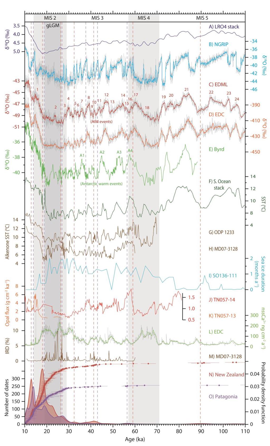
214 193

215 Figure 7.6. A comparison of the timing of glacial advances in the southern mid-latitudes during ka (red and purple dashed vertical lines) from our compiled 10 Be chronology (N and O) with a range of other palaeoclimatic proxies. (A) The LR04 benthic foraminiferal stack from Lisiecki & Raymo (2005), which shows a combined signature of global temperature and ice volume. (B) The NorthGRIP (NGRIP) ice core δ 18 O record from Greenland as a proxy for North Atlantic temperature changes (Rasmussen et al., 2006). (C) The East Dronning Maud Land (EDML) ice core δ 18 O record (EPICA, 2006), (D) the EPICA Dome C (EDC) ice core δd record (EPICA, 2006) and (E) the Byrd ice core δ 18 O record (Blunier & Brook, 2001) as proxies for Antarctic temperature changes from different parts of the ice sheet. The NGRIP, EDML and EDC records are shown on the AICC2012 common timescale (Veres et al., 2013), whereas the Byrd ice core is plotted on its own timescale. (F) The Southern Ocean Sea Surface Temperature (SST) Stack of Barrows et al. (2007) as a proxy for broad SST change around New Zealand. (G and H) The alkenone-derived SST reconstructions of Kaiser et al. (2005) for ODP-1233 off the western coast of northern Patagonia and Caniupan et al. (2011) for MD off the western coast of southern Patagonia, both plotted on the same scale. (I) A diatom-based reconstruction of sea ice extent from south of the Sub-Antarctic Front by Crosta et al. (2004), measured as the number of months per year that sea ice covered site SO (J and K) Records of opal flux from two cores in the South Atlantic, south of the Polar Front, as a proxy for wind-driven upwelling (Anderson et al., 2009). Note that the scales are different. (L) Ca 2+ flux as recorded in the EDC ice core as a proxy for dust deposition over Antarctica, thought to be sourced predominantly from Patagonia. (M) A record of Ice-Rafted Debris (IRD) from core MD (Caniupan et al., 2011). Following page Figure 7.7. As per Figure 7.6, but scaled to cover just ka. 194

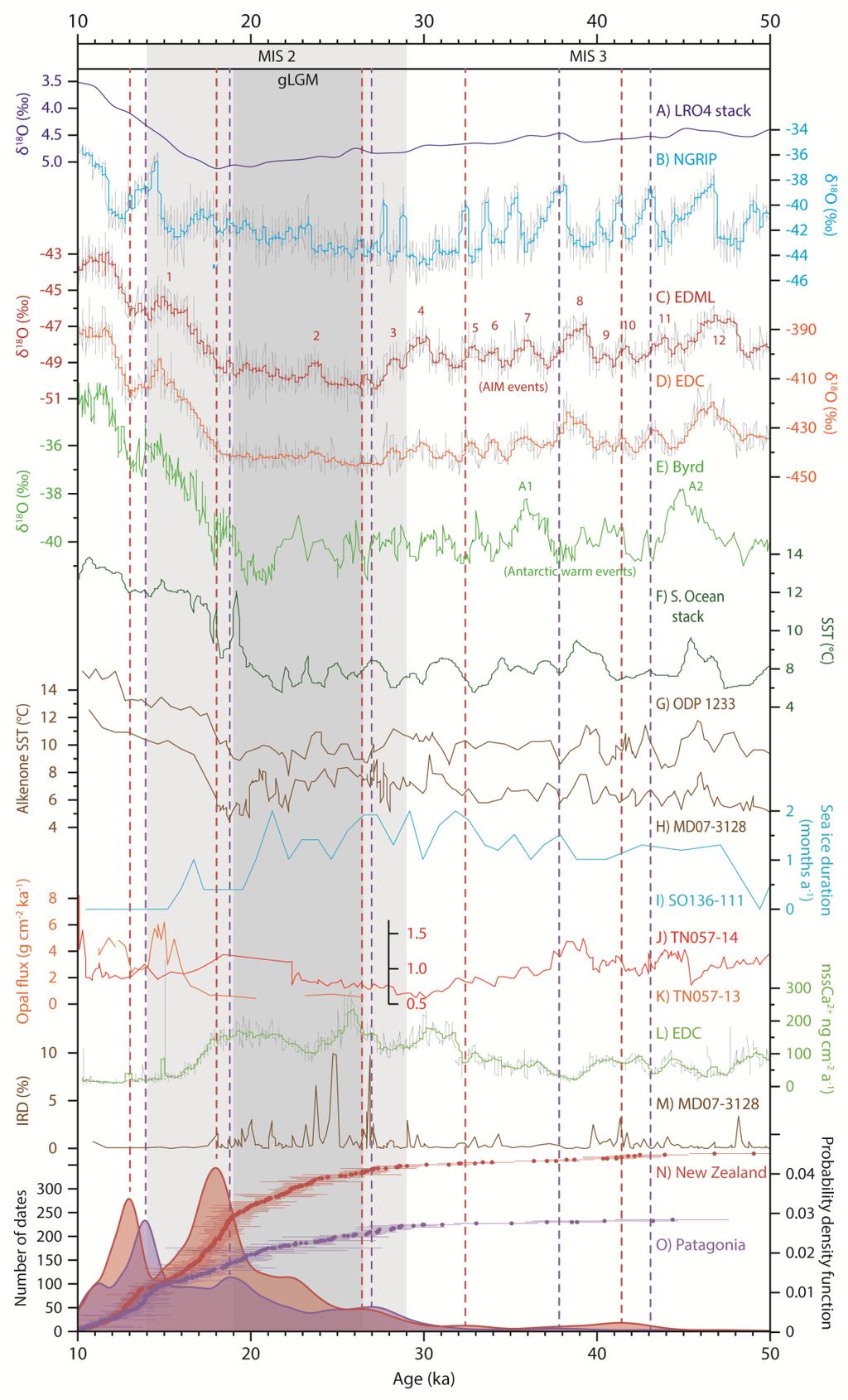
216 195

217 Ice core temperature changes Ice core temperature records from Antarctica and Greenland can help to illustrate interhemispheric climate (a)synchrony during the last glacial cycle (EPICA, 2006; Barker et al., 2009; Wolff et al., 2009; Wolff et al., 2010b; Stenni et al., 2011). Similarities between Antarctic ice core records and the Patagonia and New Zealand glacial advances would support the idea that temperature changes drove glacial advances, and operated across the southern mid-high latitudes. Broadly speaking, the EDML (EPICA, 2006), EDC (EPICA, 2004; 2006) and Byrd (Blunier & Brook, 2001) ice cores from Antarctica, and North GRIP (NGRIP; Rasmussen et al., 2006) ice core from Greenland, demonstrate a pattern of cooling through the last glacial cycle, with peak warmth during MIS 5 followed by a deterioration during MIS 4, warmer but decreasing temperatures during MIS 3, and peak cooling during MIS 2 (the glgm), before warming into the Holocene (Figures 7.6 and 7.7). In the Antarctic cores, warming events during MIS 4 and MIS 3 (A1-4) were proposed by Blunier & Brook (2001) and have been correlated to similar events in the southern mid-latitudes (Lamy et al., 2004; Barrows et al., 2007a). Additional Antarctic Isotope Maxima (AIM) events, identified in the EDML core (EPICA, 2006), occur between A1-4 and appear to coincide with Dansgaard- Oeschger (D-O) events in NGRIP, implying that hemispheric climate changes occurred broadly in phase during much of the last glacial cycle (EPICA, 2006; Wolff et al., 2009). This system broke down during the last glacial termination, where warming in the Antarctic ice cores was not followed by an abrupt warming in Greenland, resulting in continued warming in the south (Lamy et al., 2007; Wolff et al., 2009). Taken together, the ice core records show broadly consistent global climatic changes throughout the last glacial cycle but also highlight short fluctuations which may represent short-lived temperature changes propagated across the southern hemisphere that could have induced glacier advances Sea surface temperature changes Marine core records can be used to reconstruct more localised sea surface temperatures (SST) over time using microfaunal assemblages (e.g. foraminifera or diatoms) or geochemical alterations (e.g. Mg/Ca ratios from foraminifera or UK 37). This can help to show how oceanic fronts (which control surface temperature gradients) migrated over time. On the hemispheric level, similarities between SST and ice core temperature records would imply that temperature changes operated 196

218 across the Southern Hemisphere. Regionally, similarity between SST reconstructions implies that they were bounded by the same frontal systems, whereas significant difference suggests they were separated by an oceanic front, causing a significant difference in temperature. Mid-latitude glaciers are likely to have responded to cooler local SST changes. Alkenone SST records from the south-eastern Pacific, close to the western margin of the northern Patagonian Ice Sheet, have been reconstructed from core ODP (Lamy et al., 2004; Kaiser et al., 2005; Lamy et al., 2007), and can be compared with the Barrows et al. (2007a) Southern Ocean SST stack, which is a good representation of SST changes off New Zealand (Figures 7.6 and 7.7). The stack is an average of an Mg/Ca SST record from core MD from south of New Zealand (Pahnke et al., 2003) and a faunal-based SST record from core MD from the Indian Ocean (Labeyrie et al., 1996). These SST records show patterns of temperature change similar to the Antarctic ice cores across the last glacial cycle (Barrows et al., 2007a; Putnam et al., 2013b). However, numerous SST reconstructions suggest that the decline towards peak glacial temperatures had started by at least 30 ka in the south-eastern Pacific (Lamy et al., 2004; Kaiser et al., 2005; Lamy et al., 2007; Caniupán et al., 2011), west of New Zealand and south of Australia (Pelejero et al., 2006; Barrows et al., 2007a; Calvo et al., 2007), the Indian Ocean (Labeyrie et al., 1996), and the southeast Atlantic (Barker et al., 2009). The millennial-scale events recorded in mid-latitude SST records occur rapidly, so likely reflect changes in the position of oceanic fronts (Barrows et al., 2007a). The migration of the Sub-Tropical Front (STF) and Sub-Antarctic Front (SAF) over time would have altered SSTs around Patagonia and New Zealand by altering heattransfer flows such as the Agulhas current off southern Africa (Barrows et al., 2007a) and the position and/or intensity of the Antarctic Circumpolar Current (ACC) and Southern Westerly Wind system, whilst influencing latitudinal SST gradients (Shulmeister et al., 2004; Kaiser et al., 2005). Lamy et al. (2007) and Denton et al. (2010) described a coupled atmosphere-ocean system in which latitudinal shifts in the STF and Southern Westerly Winds occur in response to changes in the Inter- Tropical Convergence Zone (ITCZ), driven by Northern Hemisphere sea ice extent, and changes in the sea ice extent around Antarctica. Several records suggest northward migration of oceanic fronts during globally cooler periods that resulted in reduced SSTs around Patagonia and New Zealand. In the southwest and central Pacific, the STF may have migrated 1-2 (Sikes et al., 2009) or more, whilst in the southeast Pacific the STF and SAF may have shifted substantially more, by as 197

219 much as 5-6 during MIS 2 (Gersonde et al., 2005; Kaiser et al., 2005; Caniupán et al., 2011). In both regions, this could have resulted in reasonably rapid changes in SST, triggering terrestrial cooling and glacial advances. In summary, SST records show broadly similar patterns of temperature change to the Antarctic ice core records, indicating hemispheric propagation of climate change over the last glacial cycle. However, SSTs had deteriorated by ca. 30 ka, earlier than Antarctic temperatures, which may have been due to northward migration of the oceanic fronts Sea ice The build-up of sea ice may respond to northward migration of the Southern Westerly Winds and Antarctic Circumpolar Current, but also likely triggers these processes by altering overturning circulation and hence SST gradients. Unpicking the cause and effects within this system is challenging, but comparing sea ice records with the timing of glacial advances can at least help in evaluating whether there is a relationship between sea ice changes and the terrestrial realm. We might anticipate sea ice to generally reflect cooler conditions, and therefore increase at the same time that glaciers in Patagonia and New Zealand advanced. A reconstruction from south of the Polar Front by Crosta et al. (2004) suggests that sea ice duration increased markedly after ca. 78 ka until ca. 15 ka, with peak duration between ca. 32 and 21 ka, in a pattern consistent with decreasing temperatures in Antarctica. This pattern was developed further using diatom reconstructions from a core transect in the southwest Atlantic, east of the Drake Passage (Gersonde et al., 2003; Allen et al., 2011). Maximum summer sea ice extent around Antarctica occurred between ca. 30 ka and 22 ka, prior to the glgm, but it had retreated to south of 61 S by ca. 22 ka, although winter sea ice did not retreat until ca. 19 ka, causing a large expanse of seasonally open waters within the Scotia Sea from 22 ka onwards (Allen et al., 2011). Antarctic sea ice has been invoked in several explanations for global climate change during the last glacial cycle (Allen et al., 2011). It is likely that increased sea ice would have increased deep water formation and expansion (Seidov & Maslin, 2001; Ferrari et al., 2014) and promoted stratification of the Southern Ocean due to freshening of the surface waters (Putnam et al., 2013b). Sea ice extent is also likely to have been reduced by a southward shift of the Southern Westerly Winds and oceanic fronts, helping to destabilise any stratification of the Southern Ocean. 198

220 There is, then, a potentially important link between Antarctic sea ice and global glacial-interglacial climate change (Denton et al., 2010), and an intrinsic link between sea ice and Southern Ocean stratification (Putnam et al., 2013b) Upwelling Upwelling of CO 2 in the Southern Ocean can be reconstructed using records of opal flux. For example, Anderson et al. (2009) used records from cores TN057-13PC and -14PC to show that productivity south of the Polar Front was linked to upwelling of deep water masses during the last glacial cycle, driven by increased wind stress on the surface ocean. Upwelling broadly increased and decreased during episodes of warming and cooling, respectively, including the Antarctic A events. Thus, upwelling reached a minimum as sea ice extent peaked, likely due to stratification of the Southern Ocean (Putnam et al., 2013b), and we would anticipate increased upwelling during cooler periods. The Southern Ocean may have entered a fully stratified state by ca. 70 ka (Anderson et al., 2009), consistent with the build-up of Antarctic sea ice at this time (Crosta et al., 2004), and possibly linked to increased winter duration (Putnam et al., 2013). Greater sea ice extent would not only have promoted stratification but would have pushed the oceanic fronts in the Southern Ocean further north, creating stronger SST gradients and triggering northward migration of the Southern Westerly Winds, further increasing sea ice expansion and reducing upwelling. This model, advocated by Denton et al. (2010) and Putnam et al. (2013b), amongst others, provides a theoretical link between sea ice formation, STF, SAF and Southern Westerly Wind migration, and SST changes around Patagonia and New Zealand. Thus, records of upwelling in the Southern Ocean suggest that it broadly followed global warming and cooling during the last glacial cycle linked to stratification of the water column. However, the ocean may have been partially or fully stratified by ca. 70 ka, which would have forced oceanic frontal systems northwards Summary of last glacial cycle time periods Late MIS 5 (ca ka) There is little evidence for glacial advances during MIS 5, apart from occasional dates from individual glaciers, such as around 90 ka (Sutherland et al., 2007; Glasser et al., 2011), supported by low dust concentrations in the EDML ice core at this time and low sea ice extent (Fischer et al., 2007). Antarctic temperatures were warmer, though with millennial-scale variability including a cooler period between ca. 199

221 92 ka and 87 ka (EPICA, 2006). Temperature changes were similar to Greenland, but it is unclear precisely whether the hemispheres were in-phase or out-of-phase. Localised records suggest that warmer SSTs followed Antarctic temperature changes (Barrows et al., 2007a), including the millennial-scale variability and the marked cooler period between 92 ka and 87 ka. Hemispheric temperature changes followed Northern Hemisphere summer insolation (Berger & Loutre, 1991), and winter duration in the Southern Hemisphere increased between 105 ka and 95 ka (Huybers & Denton, 2008), with no major latitudinal offset in seasonality. Whilst a cooler period between 92 ka and 87 ka could have triggered glacial advances in Patagonia and New Zealand, overall MIS 5 was not likely to have promoted ice sheet expansion in either region MIS 4 (ca ka) There is limited evidence for glacial advances during MIS 4, although scattered dates suggest that some glaciers expanded during this time, supported by increases in dust production and sea ice extent (Wolff et al., 2006; Fischer et al., 2007) and a reduction in upwelling (Anderson et al., 2009). Antarctic temperatures showed a marked cooling with a cold period equivalent to the glgm in temperature in both Antarctic and Greenland ice cores until around 63 ka (EPICA, 2006; Rasmussen et al., 2006). There was a similar drop in localised SST records around New Zealand (Barrows et al., 2007a), likely due to northward migration of the STF (Sikes et al., 2009). An even greater SST reduction occurred off the west coast of northern Patagonia, where temperatures reached their lowest levels during the last glacial cycle due to a 5-6 northward shift of the STF (Kaiser et al., 2005). Northern Hemisphere summer insolation was increasing, but Southern Hemisphere summer insolation was decreasing (Berger & Loutre, 1991), and there was a period of longer duration winters just prior to MIS 4 (Huybers & Denton, 2008) followed by a period of decreased seasonality. Therefore, the evidence suggests that MIS 4 was a major cool period in the southern mid-latitudes, and should have instigated significant glacial advances. The absence of dates in our compilation either suggests that any glacial activity was not as extensive as later advances or MIS 4 moraines have not yet been sampled Early MIS 3 (ca ka) There are only scattered dates from New Zealand during early MIS 3, and dust and IRD records show little activity beyond occasional small peaks (Fischer et al., 2007; Caniupán et al., 2011). The limited evidence does align in places, notably between 200

222 ca. 50 ka and 46 ka (Antarctic warming events A3 and A2), and may suggest that ice advances occurred but were of limited extent or have not been sampled. Overall, Antarctic temperatures warmed following MIS 4 (EPICA, 2006), though not as much as MIS 5 or MIS 1, and the rest of early MIS 3 showed a strong millennial-scale pattern of warming and cooling into and out of the A4-1 events (Blunier & Brook, 2001), broadly covarying with D-O events in Greenland (Rasmussen et al., 2006; Wolff et al., 2010b). These events are propagated into local SST changes, causing significant variability of up to 3 C that could have been caused by fluctuating shifts in the oceanic fronts (Barrows et al., 2007a; Caniupán et al., 2011). The absence of prolonged cooling or build-up of sea-ice (Crosta et al., 2004; Wolff et al., 2006) suggests that these were only transient events and probably prevented any significant glacial advances, supported by decreasing, but variable, upwelling in the Southern Ocean (Anderson et al., 2009). Northern Hemisphere summer insolation peaked and then started to decrease during this time, and Southern Hemisphere summer insolation peaked alongside increasing seasonality (Berger & Loutre, 1991). The implication is that while millennial-scale events may have caused some glacial activity that is not well recorded in our compilation (e.g. between 50 ka and 46 ka), overall climatic conditions were not well suited for glacial advances during MIS Late MIS 3 (ca ka) There is good evidence for glacial advances during late MIS 3, at 43.1 ka and 37.8 ka in Patagonia, and 41.4 ka and 32.4 ka in New Zealand. This is marked by small peaks in IRD and dust flux (Fischer et al., 2007; Caniupán et al., 2011), though the latter increases towards the end of the period. Antarctic ice cores show a subtle cooling trend that is heavily overprinted by millennial-scale variability, including the A1 event, the cool periods of which broadly align with glacial advances (Blunier & Brook, 2001; EPICA, 2006; Wolff et al., 2009; Wolff et al., 2010b; Kelley et al., 2014). Local SST records suggest that average temperatures had reached values similar to MIS 2 by this time, although Antarctic millennial-scale variability continued to be propagated across the mid-latitudes, likely related to continued fluctuations in the STF (Lamy et al., 2004; Kaiser et al., 2005; Barrows et al., 2007a). Significantly, there was a marked increase in Antarctic sea ice at this time (Crosta et al., 2004; Allen et al., 2011), correlating with a reduction in upwelling in the Southern Ocean (Anderson et al., 2009), which reached a minimum in the last glacial cycle at 30 ka. Northern Hemisphere insolation was slowly decreasing towards MIS 2 and, whilst Southern Hemisphere winter duration increased over the whole of MIS 3, there was 201

223 a switch to more rapidly increasing winter duration from ca. 36 ka (Huybers & Denton, 2008), which occurred whilst Southern Hemisphere insolation and seasonality both decreased between ca. 45 ka to 30 ka. In short, climatic conditions in the southern mid-latitudes were well suited for glacial advances during late MIS 3. Longer duration winters, decreasing summer insolation and decreasing seasonality promoted ice growth and were enhanced by fluctuations in the oceanic fronts, periodically delivering cooler temperatures to Patagonia and New Zealand. This was likely in tandem with increases in sea ice extent which reduced upwelling by stratifying the Southern Ocean and forcing the SAF, STF and Southern Westerly Winds further north to deliver cooler and wetter conditions to more of the glaciers (Putnam et al., 2013b) MIS 2 (ca ka) and the glgm period ( ka) There were clear glacial advances either side of the glgm at 27.0 ka and 18.8 ka in Patagonia and 26.4 ka and 18.0 ka in New Zealand. These correlate with major peaks in IRD and dust flux during early MIS 2 (Fischer et al., 2007). However, whilst dust levels remained relatively high, IRD reduced markedly through the glgm, perhaps due to a retreat of marine-terminating glaciers (Caniupán et al., 2011). The advances occurred at the very start and end of a period of intense cooling in Antarctica, similar to that in Greenland, and at the same time that significant millennial-scale variability ended in Antarctica (EPICA, 2006; Rasmussen et al., 2006). This suggests that glaciers responded rapidly to a drop in Southern Hemisphere temperatures at around 27.5 ka, perhaps because they had already advanced during late MIS 3, and then did not advance in unison again until the very end of the cool period. Local SST records suggest a continuation of the cooler temperatures from late MIS 3 (Lamy et al., 2004; Kaiser et al., 2005; Barrows et al., 2007a), with no marked change except for off the west coast of southern Patagonia where proximal ice melt likely caused enhanced cooling of surface waters (Caniupán et al., 2011). The advances at 18.8 ka and 18.0 ka align with a severe reversal in warming in SST around New Zealand (Barrows et al., 2007a), suggesting that the STF may have fluctuated rapidly: first southward, then northward, then southward again. This may have altered both the local temperature and precipitation regimes, triggering a glacial advance despite no obvious drop in hemispheric temperature. Other frontal reconstructions have suggested that the STF and SAF migrated northwards by 1-2 around New Zealand (Sikes et al., 2009) and 5-6 around Patagonia (Kaiser et al., 2005), although this likely happened during late MIS 3. Sea ice extent remained relatively high from late MIS 3, but reduced markedly 202

224 after ca. 20 ka, with an associated increase in upwelling (Crosta et al., 2004; Anderson et al., 2009; Allen et al., 2011). This was a period of reduced summer insolation in the Northern Hemisphere (Berger & Loutre, 1991), and the large northern ice sheets responded by reaching maximum extents. In the Southern Hemisphere, summer insolation increased and peaked at around 21 ka, and seasonality increased, with a latitudinal offset from ca. 30 ka. Overall, conditions during much of MIS 2 were not as well suited for glacial advances as late MIS 3: summer insolation and seasonality increased; winter duration decreased; local SSTs did not decrease further; and IRD, dust flux and Antarctic sea-ice reduced significantly. Stratification may have deteriorated with southerly migration of the STF, SAF and Southern Westerly Winds. Glacial advances were likely still recorded only because global temperatures reached a minimum around the glgm, indicated by a prolonged cooling in Antarctica without substantial millennial-scale variability. Advances towards the end of MIS 2 may have been triggered by northward fluctuations of the STF, providing cooler temperatures and increased precipitation at a time when most other factors suggest deglaciation had already started in the southern mid-latitudes The late-glacial period (ca ka) Our compilation suggests that glaciers advanced during the Antarctic Cold Reversal at 13.9 ka in Patagonia and 13.0 in New Zealand. The absence of evidence for advances in the IRD or dust records suggests that the advance was either weak or, more probably, a prolonged stillstand. Antarctic temperatures decreased at this time, in antiphase with a warm period in Greenland and thus prior to the Younger Dryas (EPICA, 2006; Rasmussen et al., 2006). This temperature drop only registers as a plateau in warming in the local SST records (Caniupán et al., 2011), supporting a minimal advance of glaciers at this time. Northern Hemisphere insolation was increasing and Southern Hemisphere insolation was decreasing (Berger & Loutre, 1991), but the sub-orbital timescale of the late glacial events suggests that they were not related to changes in insolation intensity. Sea ice does not seem to have expanded significantly, but there is an apparent drop in upwelling (Anderson et al., 2009), which could indicate northern migration of the Southern Westerly Winds and oceanic fronts, triggering a slowdown in the recession of glaciers in Patagonia and New Zealand. This may have also caused the offset in timing between Patagonia and New Zealand, given that higher latitude glaciers would have benefitted first from a northward migration of precipitation. The effect on SSTs in northern Patagonia and 203

225 New Zealand (Lamy et al., 2004; Barrows et al., 2007a) compared to southern Patagonia (Caniupán et al., 2011) supports the assertion that the stillstand was driven by movement of the coupled oceanic-atmospheric frontal system, rather than by hemisphere-wide cooling. 7.5 Conclusions The first compilation of previously published 10 Be exposure dating for Patagonia and New Zealand suggests that glaciers advanced at various times throughout the last glacial cycle, supported by similar evidence from radiocarbon dating. There is commonality in the timing of glacial advances between numerous glaciers in both Patagonia and New Zealand, and we infer this to represent periods of broad, regional glacial advances. However, this does not mean that all glaciers advanced synchronously and does not provide information on the extent of the glacial advances. That said, the chronologies from Patagonia and New Zealand show remarkable similarities, suggesting that similar forcing factors may have been influencing both ice sheets during the last glacial cycle. In particular, both regions show a trend for glacial advances, replicated in different glaciers, from at least 45 ka, with advances at ca ka, ka, ka, ka and ka. In general, our compilation reveals a number of significant characteristics in the timing of glacial advances in the southern mid-latitudes. Glaciers were advancing well before the glgm, and indeed by the latter half of MIS 3, with two advances prior to 30 ka. Further advances were concentrated just before and after (but not during) the glgm, and late glacial advances or stillstands in Patagonia and New Zealand occurred during the Antarctic Cold Reversal, rather than the Younger Dryas. Future work should target glacial limits beyond those dated to the glgm. In particular, an absence of dated limits from MIS 4 is puzzling given that numerous proxy records suggest that this period resulted in significant climate deterioration in the southern mid-latitudes. There is no clear correlation between a single climatic forcing factor and the advances we identify. Rather, the forcing factors responsible likely changed over time. Our study suggests that ice sheet expansion in Patagonia and New Zealand was driven by underlying orbital parameters, involving a combination of summer intensity, seasonality, and winter duration, but that the precise timing is likely to have been intrinsically linked to migration of the coupled ocean-atmosphere system. Evaluating the various factors likely to have affected the timing of southern midlatitude glacial advances suggests that late MIS 3 experienced optimum conditions 204

226 for glaciers to have advanced. Summer insolation reached a minimum, seasonality was reduced, winter duration was increasing, and sea ice had expanded significantly. This may have induced stratification of the ocean and triggered northward migration of the STF and SAF, bringing cooler temperatures to more of Patagonia and New Zealand and inducing an equatorward shift in the moisturebearing Southern Westerly Winds system. Hence, whilst global temperatures did not reach a minimum until MIS 2, summer insolation in the Southern Hemisphere was much higher by that time, and Antarctic sea ice reduced markedly, possibly aided by southward migration of the coupled ocean-atmosphere frontal system as sea ice expansion in the Northern Hemisphere induced a southward shift of the ITCZ. Glacial advances during MIS 2 in Patagonia and New Zealand occurred rapidly with the onset of a prolonged globally cool phase across the glgm, marked by a discontinuation of hemispheric millennial-scale variability. A consistent offset after 30 ka, in which Patagonian glaciers advanced before those in New Zealand, is unlikely to be an artefact of age calculation but could instead relate either to a latitudinal offset in the timing of changes in seasonality between ca. 30 ka and 18 ka, or a lag related to the latitudinal migration of the coupled ocean-atmosphere system. Either way, shifts in the oceanic fronts and atmospheric circulation, as part of a complex climate feedback system, are likely to have been pivotal in determining when mid-latitude glaciers advanced during the last glacial cycle. 205

227 Chapter 8. Conclusions and implications 206

228 8.1 Key conclusions This thesis set out to reconstruct glacial changes of the southernmost ice lobes of the Patagonia Ice Sheet during the Quaternary. Specifically, the aims were to test whether ice advances occurred over timescales of 10 4, 10 5 or 10 6 years and to use this new chronological framework to examine the controls on glacial change. This work has produced a new glacial geomorphological map for the area (Chapter 3); examined the geomorphology of erratic boulder trains used for previous dating (Chapter 4); and applied cosmogenic nuclide dating of outwash depth profiles to test the age of glacial limits (Chapter 5). The thesis also presented a new glacial history for the southernmost ice lobes, against which the timing and nature of ice advances were examined (Chapter 6), and a large dating compilation from across Patagonia and New Zealand to examine possible forcing mechanisms of glacial change (Chapter 8) Objective 1: Mapping of glacial limits Mapping of glacial landforms associated with the five southernmost ice lobes showed eleven types of glacial landform: moraine ridges, subdued moraine topography, kettle-kame topography, glacial lineations, irregular and regular hummocky terrain, irregular dissected ridges, an esker, meltwater channels, former shorelines and outwash plains. The geomorphological map reveals the dominance of meltwater landforms (channels, outwash plains and kettle-kame topography) in the study area. It also highlights a difference in the nature of landforms associated with the northern three ice lobes, where limits are marked by numerous clear moraine ridges, compared to those to the south, where hummocky terrain and drift limits prevail. In places, the analysis demonstrated cross-cutting relationships indicative of re-advances Objective 2: Use of erratic boulder trains for dating Erratic boulder trains have been used to provide cosmogenic nuclide dates that have proven critical in the discussion of the timing of glacial advances in the region. Several boulder trains along the southern edge of the BI-SSb lobe have been previously hypothesised to have been deposited in different glacial cycles, even though exposure dating yielded ages within the last glacial cycle. A detailed examination of the boulders in this thesis suggested that they were produced by one or more supraglacial rock avalanches. Rock surface weathering analysis showed little difference in the weathering characteristics between the boulder trains, which is 207

229 interpreted to indicate that the EBTs are closer in age than previous work has implied. Thus, while erratic boulder trains can provide useful flow-line indicators and sources of cosmogenic nuclide exposure dating, it is important to understand their formation, transport, and deposition. Importantly, occasional, anomalously old dates should be expected from supraglacial boulder trains caused by pre-exposure prior to and during glacial transport Objective 3: Depth profile dating of key limits Ultimately, testing the age of glacial limits in the region requires new, independent dating to provide robust ages not compromised by post-depositional processes. In light of the new mapping and analysis of the erratic boulder trains, cosmogenic 10 Be and 26 Al exposure dating of depth-profiles was conducted through outwash associated with the Río Cullen and San Sebastián glacial limits of the BI-SSb lobe, previously hypothesised to date to MIS 12 and 10, respectively. The limits formed more recently than previously thought, giving ages of 45.6 ka (+139.9/-14.3) for the Río Cullen, and 30.1 ka (+45.6/-23.1) for the San Sebastián limits. These dates indicate extensive glaciation in southern Patagonia during MIS 3, prior to the wellconstrained, but much less extensive MIS 2 (glgm) limit that has been dated using cosmogenic dating of boulders and other independent chronological techniques. Whilst the errors from the depth-profile technique are large due to a conservative approach, and large scatter in boulder ages does not allow precise constraint on the timing of deposition of these glacial limits, all of the evidence points towards glacial advances during the last glacial cycle rather than numerous glacial cycles over hundreds of thousands of years Objective 4: Reconstructing the regional glacial history The new age constraints for the BI-SSb lobe warranted further investigation into the timing and nature of ice advances of the five southernmost ice lobes. The geomorphological mapping was used to reconstruct former glacial limits, demarcate flowsets from landform assemblages, reconstruct former proglacial lakes, and evaluate possible glacial landsystems represented in the region. Eight time steps were reconstructed, which highlight the dynamic nature of these ice lobes. There is good evidence for rapid ice flow in the region, and possible surge-like activity, particularly in the Otway and Magellan lobes. Most of the ice lobes re-advanced on at least one occasion and there is evidence for potentially catastrophic drainage of the palaeo-laguna Blanca proglacial lake. The relative history was used to reexamine published chronological data for the ice lobes, which suggested that the 208

230 Magellan, Otway and Skyring lobes likely advanced prior to the glgm, in a manner similar to the BI-SSb lobe, with similar limits around 30 ka in several of the ice lobes. More extensive limits may have been deposited during the last glacial cycle or during earlier glacial stages in the Quaternary. The evidence for dynamic ice advance and retreat highlights that climatic reconstructions from the glacial geomorphology are not straightforward. However, the similarity in timing elucidated from the available chronological evidence suggests that an underlying external likely climatic forcing factor controls glacial advances Objective 5: Examining southern mid-latitude glaciation To examine the possible climatic forcing factors further, a large dataset of previously published 10 Be exposure dates from Patagonia and New Zealand was compiled. This shows that glaciers across a broad range of the southern mid-latitudes advanced at various times during the last glacial cycle. Commonality in the timing of glacial advances implies periods of broad, regional glacial advances driven by similar forcing factors, although this does not mean that all glaciers advanced synchronously. Both regions show a trend for glacial advances, replicated in different glaciers, from at least 45 ka, with advances at ca ka, ka, ka, ka and ka. Thus, glaciers were advancing well before the glgm, and indeed by the latter half of MIS 3. The glacial advances were likely driven by underlying orbital parameters, involving a combination of summer intensity, seasonality and winter duration. However, the precise timing is likely to have been linked to the migration of the coupled ocean-atmosphere system. Late MIS 3 may have experienced optimum conditions for glaciers to have advanced: minimum summer insolation, reduced seasonality, increasing winter duration, and expanded sea ice. Ocean stratification and northward migration of the STF and SAF, would have brought cooler temperatures to more of Patagonia and New Zealand and induced an equatorward shift in the moisture-bearing Southern Westerly Wind system. 8.2 Implications The main implication of this work is that during the last glacial cycle, extensive glacial advances occurred in southernmost South America prior to the glgm. This is contrary to the established age model for the timing of glacial advances in Patagonia, but is supported by a compilation of dating evidence from the rest of Patagonia and New Zealand, which suggests that glacial advances during MIS 3 may have been a common feature across the southern mid-latitudes. This finding is 209

231 important because it suggests that previous work on glacial chronologies around the world may have missed similar advances during the last glacial cycle. It also adds to a growing body of work that shows that glaciers in the southern mid-latitudes advanced prior to the glgm and did not, therefore, follow global climate trends in the same way as large ice sheets in the Northern Hemisphere. The conclusions and implications of this thesis lead to a number of potential areas for future research Further work Dating of the Río Gallegos, Skyring and Otway lobes The Río Gallegos, Skyring and Otway lobes remain broadly undated. Chapter 6 demonstrated an age of ca. 30 ka for a pre-glgm limit across the Magellan, Otway and Skyring lobes, but the glacial chronology could be significantly extended. An absence of boulders on moraines has likely hindered previous dating attempts, but Chapter 5 highlighted the suitability of depth profiles in outwash for dating glacial limits of the BI-SSb lobe, and this would be worth pursuing for the other southernmost ice lobes if suitable sampling locations can be found Palaeo-Laguna Blanca drainage Chapter 6 reconstructed a significant lake drainage event associated with palaeo- Laguna Blanca, first identified by Lovell et al. (2012). Given the need for new dates, and the suitability of outwash plains for dating glacial limits in the region, this would be an excellent target. An age from sediments relating to the lake drainage would also help to constrain the timing of the pre-glgm limits of the Skyring and Otway lobes suggested to have been deposited at ca. 30 ka in Chapter Ice thickness constraints The reconstruction in Chapter 6 provides useful information on glacial extent over time, but cannot say anything about ice thickness. Improved ice thickness estimates would allow palaeoclimatic modelling from the glacial geomorphological record, so this would make a useful addition to our reconstruction. Data on ice thickness would be best provided by identifying and dating trimline evidence, similar to Boex et al. (2013) for northern Patagonia Investigations into possible palaeo-surges Chapter 6 presented evidence for possible surge-like behaviour of the BI-SSb, Magellan and Otway lobes, but this was based predominantly on discontinuous landform evidence, and none of the lobes display ideal surging landform suites. 210

232 This initial, tentative work requires further investigation and would benefit from more detailed sedimentological work to assess features such as glaciotectonised moraines and crevasse-fill ridges. Work on glacial surges has largely been confined to contemporary systems, so palaeo-examples could help to improve our understanding of their triggers in relation to long-term climate and/or topography Sedimentological work As mentioned above, the landsystem approach adopted in Chapter 6 was necessarily tentative. This thesis was primarily concerned with glacial chronology and reconstructing broad glacial changes from landforms, but sedimentological work would help to improve our understanding of former glacial dynamics across the region, in a similar manner to the localised work of Benn & Clapperton (2000a; b) Dating pre-glgm moraines in Patagonia Chapter 5 demonstrated that glacial limits thought to date from MIS 12 and 10 were deposited during the last glacial cycle. This may not have been anomalous, and similar limits could have been deposited across Patagonia. Indeed, work by Glasser et al. (2011) has already suggested the presence of limits of similar age to the BI- SSb lobe in the San Martín Valley. Thus, moraines beyond the glgm limits in the rest of Patagonia could be targeted for dating to better resolve any regional differences associated with the migration of oceanic and/or atmospheric fronts MIS 4 in Patagonia As noted in Chapter 7, the absence of glacial advances during MIS 4 is puzzling given that other palaeoclimatic records indicate significant climate deterioration at this time. Moraine chronologies in Patagonia could be re-examined to establish if MIS 4 moraines have been missed or whether they are truly absent from the southern mid-latitudes Ice sheet modelling Modelling of the Patagonian Ice Sheet needs to be updated to reflect our increased understanding of the timing and nature of ice advances. Modelling power has advanced significantly since the last full ice sheet model by Hulton et al. (2002), and this thesis has provided a rigorous glacial reconstruction against which ice sheet models can be compared. In this way, our understanding of past climate change in southernmost South America can be improved further. 211

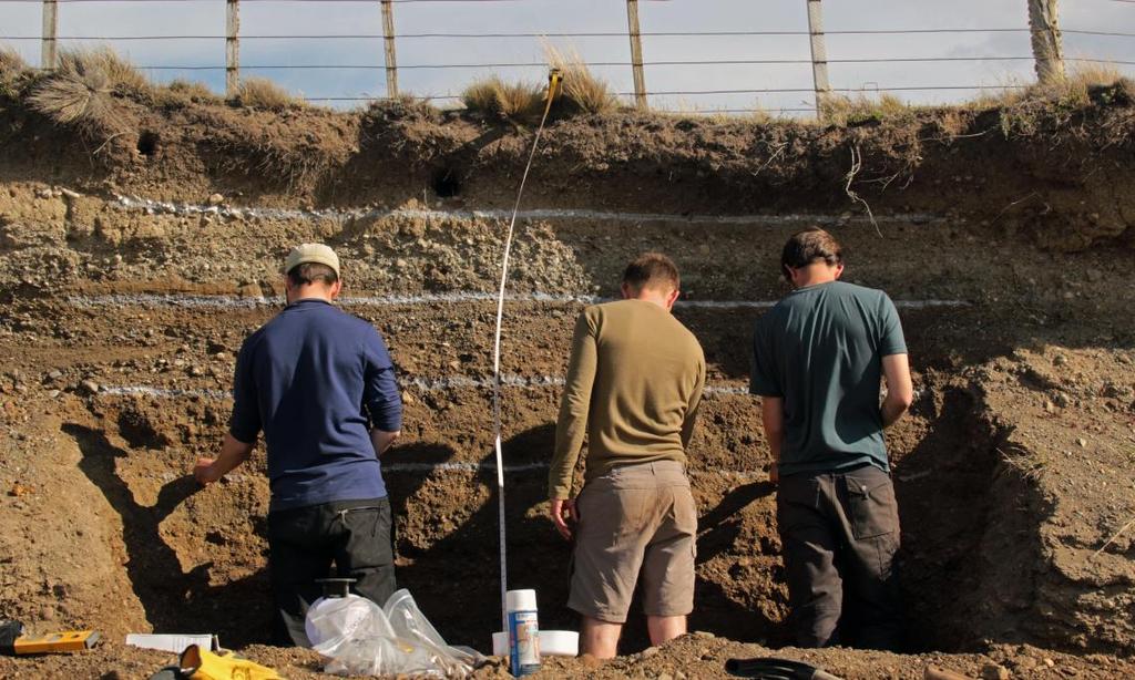
233 212