Edge Detection in Computer Vision Systems

Transcription

1 1 CS332 Visual Processing in Computer and Biological Vision Systems Edge Detection in Computer Vision Systems This handout summarizes much of the material on the detection and description of intensity changes in images that will be discussed in class. General Points: Physical changes in the scene, such as the borders of objects, surface markings and texture, shadows and highlights, and changes in surface structure, give rise to changes of intensity in the image. The first step in analyzing the image is to detect and describe these intensity changes they provide the first hint about the structure of the scene being viewed. It is difficult to identify where the significant intensity changes occur in a natural image. The raw intensity signal can be very complex, with changes of intensity occurring everywhere in the image and at different scales. We will consider one common approach to the detection of intensity changes that incorporates three basic operations: smoothing, differentiation and feature extraction. Two of these operations, smoothing and differentiation, can be combined into a single processing step. Below is a small portion of an image taken with a digital camera, showing the image intensity at each location. The indices of the rows and columns of the array containing this image are indicated along the top row and left column. The full image contains a bright circle against a dark background, and the sample below shows a small portion of the upper left region of the circle. A contour is drawn through the array indicating the border between the bright circle (lower right) and dark background (upper left). IMAGE

2 2 The purpose of the smoothing operation is to remove minor fluctuations of intensity in the image that are due to noise in the sensors, and to allow the detection of changes of intensity that take place at different scales. In the image of a handi-wipe cloth (shown later), for example, there are changes of intensity taking place at a fine scale that correspond to the individual holes of the cloth. If the image is smoothed by a small amount, the variations of intensity due to the holes are preserved. At a coarser scale, there are intensity changes that follow the pattern of colored stripes on the cloth. If the image is smoothed by a greater amount, the intensity fluctuations due to the holes of the cloth can be smoothed out, leaving only the larger variations due to the stripes. The purpose of the differentiation operation is to transform the image into a representation that makes it easier to identify the locations of significant intensity changes. If a simple step change of intensity is smoothed out, the first derivative of this smoothed intensity function has a peak at the location of the original step change, and the second derivative crosses zero at this location. The peaks and zero-crossings of a function are easy to detect, and indicate where the significant changes occur in the original intensity function. The final step of feature extraction refers to the detection of the peaks or zero-crossings in the result of smoothing and differentiating the image. There are properties of these features that give a rough indication of the sharpness and contrast of the original intensity changes. Convolution: The smoothing and differentiation steps can be performed using the operation of convolution. This section provides a simplified description of the convolution operation that is adequate for how we will use convolution in practice. This operation involves calculating a weighted sum of the intensities within a neighborhood of each location of the image. The weights are stored in a separate array that is usually much smaller than the original image. We will refer to the pattern of weights as the convolution operator. For simplicity, we will assume that the convolution operator has an odd number of rows and columns so that it can easily be centered on each image location. To calculate the result of convolution at a particular location in the image, we center the convolution operator on that location and compute the product between the image intensity and convolution operator value at every location where the image and convolution operator overlap. We then calculate the sum of all of these products over the neighborhood. In the example at the top of the next page, a portion of an image is shown on the left (the array indices are again shown along the top row and left column) and a simple 3x3 convolution operator is shown on the right. The weights in the convolution operator can be arbitrary values. In this example, they are integers from 1 to 9. The result of the convolution at location (3,3) in the image is calculated as follows: C(3,3) = 1*4 + 2*9 + 3*3 + 4*5 + 5*8 + 6*7 + 7*6 + 8*1 + 9*9 = 264 In practice, we usually only compute convolution values at locations where the convolution operator can be centered and covers image locations that are all within the bounds of the image array. For the image shown below, convolution values would not be calculated along rows 1 and 5, and columns 1 and 5.

3 3 IMAGE CONVOLUTION OPERATOR The convolution operation is denoted by the * symbol. In one dimension, let I(x) denote the intensity function, O(x) denote the convolution operator and C(x) denote the result of the convolution. We can then write: C(x) = O(x) * I(x) In two dimensions, each of these functions depends on x and y: C(x,y) = O(x,y) * I(x,y) The next two sections describe the smoothing and differentiation operations in more detail, and show how a convolution operator can be constructed to perform these operations simultaneously. Smoothing: The smoothing operation blends together the intensities within a neighborhood of each image location. A greater amount of smoothing can be achieved by combining the intensities over a larger region of the image. There are many ways to combine the intensities in a neighborhood to perform smoothing. For example, we could calculate the average of the intensities within a region around each image location. Theoretical studies suggest that a better approach is to weigh the intensities by a Gaussian function that has its peak centered at each image location. This has the effect of weighing nearby intensities more heavily than those further away, when performing smoothing. Biological systems use Gaussian-like smoothing functions in their initial processing of the retinal image. In one dimension, the Gaussian function can be defined as follows: G(x) = 1 σ e x 2 2σ 2

4 4 This function has a maximum value at x = 0. In two dimensions, the Gaussian function can be defined as: G(x, y) = 1 (x 2 +y 2 ) σ 2 e 2σ 2 This function has a maximum value at x = y = 0 and is circularly symmetric. The value of σ controls the spread of the Gaussian as σ is increased, the Gaussian spreads over a larger area. A convolution operator constructed from the Gaussian function performs more smoothing as σ is increased. For both of the above definitions of the Gaussian function, the height of the central peak decreases as σ increases, but this is not important in practice. Differentiation: We noted earlier that if a simple step change of intensity is smoothed out, the first derivative of this smoothed intensity function has a peak at the location of the original step change, and the second derivative crosses zero at this location. In one dimension, we can calculate the first or second derivative with respect to x. Let D'(x) and D''(x) denote the results of the first and second derivative computations, respectively. If I(x) is also smoothed with the Gaussian function, then the combination of the smoothing and differentiation steps can be written as follows: D'(x) = d/dx [G(x) * I(x)] D''(x) = d 2 /dx 2 [G(x) * I(x)] The derivative and convolution operations are associative, so the above expressions can be rewritten as follows: D'(x) = [d/dx G(x)] * I(x) D''(x) = [d 2 /dx 2 G(x)] * I(x)

5 5 This means that the smoothing and derivative operations can be performed in a single step, by convolving the intensity signal I(x) with either the first or second derivative of a Gaussian function, shown below (the size of the second derivative is scaled in the vertical direction). The value of σ again controls the spread of these functions as σ is increased, the derivatives of the Gaussian are spread over a larger area. d dx G(x) = x x 2 σ 3 e 2σ d 2 2 dx G(x) = 1 $ x 2 2 σ 3 σ 1 ' & ) e % 2 ( x 2 2σ 2 The figure on the next page illustrates the smoothing and differentiation operations for a onedimensional intensity profile. Part (a) shows the original intensity function. Parts (b) and (c) show the results of smoothing the image profile with Gaussian functions that have a small and large value for σ. Part (d) shows the first derivative of the smoothed intensity profile in (c), and part (e) shows the second derivative of (c). The vertical dashed lines show the relationship between intensity changes in the smoothed intensity profile, peaks in the first derivative and zero-crossings in the second derivative. In two dimensions, intensity changes can occur along any orientation in the image and there are more choices regarding how to compute the derivative. One option is to compute directional derivatives; that is, to compute the derivatives in particular 2-D directions. To detect intensity changes at all orientations in the image, it is necessary to compute derivatives in at least two directions, such as the horizontal and vertical directions. Either a first or second derivative can be calculated in each direction. It is possible to first smooth the image with one convolution step, and then perform the derivative computation by a second convolution with operators that implement a derivative. Alternatively, these two steps can be combined into a single convolution step.

6 (a) original intensity profile, (b) smoothed intensity, small σ, (c) smoothed intensity, large σ, (d) 1 st derivative of smoothed intensity, (e) 2 nd derivative of smoothed intensity. The dashed lines connect the location of an intensity change in the smoothed intensity profile with a peak in the 1 st derivative and zero-crossing in the 2 nd derivative. 6

7 7 We are going to consider in detail, an alternative approach that involves computing a single, non-directional second derivative referred to as the Laplacian. This approach is motivated by knowledge of the processing that takes place in the retina in biological vision systems. The Laplacian operator is the sum of the second partial derivatives in the x and y directions and is denoted as follows: 2 I = 2 I/ x I/ y 2 Although the Laplacian is defined in terms of partial derivatives in two directions, it is a nondirectional derivative in the following sense. Suppose the Laplacian is calculated at a particular location (x,y) in the image. The 2-D image can then be rotated by any angle around the location (x,y) and the value of the Laplacian does not change (this is not true for the directional derivatives mentioned earlier). Let L(x,y) denote the result of calculating the Laplacian of an image that has been smoothed with a 2-D Gaussian function. Then L(x,y) can be written as follows: L(x,y) = 2 [G(x,y) * I(x,y)] = [ 2 G(x,y)] * I(x,y) This means that the Laplacian and smoothing operations can be performed in a single step, by convolving the image with a function whose shape is the Laplacian of a Gaussian. This function is defined as follows: 2 G = 1 % r 2 σ 2 σ 2 ( ' * e r 2 2σ 2 & 2 r 2 = x 2 + y 2 ) This function is circularly symmetric and is shaped like an upside-down Mexican hat (the figure above shows this function with its sign reversed). It has a minimum value at the location x = y = 0. Because the Laplacian is a second derivative, the features in the result of the convolution of the image with this function, which correspond to the locations of intensity changes in the original image, are the contours along which this result crosses zero.

8 8 The space constant σ again controls the spread of this function. As σ is increased, the Laplacian of a Gaussian function spreads over a larger area. A convolution operator constructed from this function performs more smoothing of the image as σ is increased, and the resulting zerocrossing contours capture intensity changes that take place at a coarser scale. The diameter of the central negative portion of the Laplacian of a Gaussian function, which we denote by w, is related to σ as shown below. We will often refer to the size of the Laplacian of a Gaussian function by the value of w. w = 2 2σ In practice, we can scale all the values of the Laplacian of a Gaussian function by a constant factor and flip its sign, without changing the locations of the resulting zero-crossing contours. To construct a convolution operator for this function, it can be sampled at evenly spaced values of x and y and the resulting samples can be placed in a 2-D array. On the next page, we illustrate a convolution operator that was constructed in this way. This operator was derived by computing samples of the following function, which differs from the Laplacian of a Gaussian function shown earlier by a constant scale factor and a change in sign: % ( 2 G = 25' 2 r2 * e & σ 2 ) r 2 2σ 2 In the example shown, σ = 2, so that the diameter w of the central region of the function, which is now positive, is 4 picture elements (pixels). The array has 11x11 elements and the center element (location (6,6)) represents the origin, where x = y = 0. The maximum positive value of the operator occurs at this location. Note that the convolution operator is circularly symmetric.

9 9 σ = 2 w = 4 CONVOLUTION OPERATOR Shown below is a portion of the result of convolving the image of the noisy circle (shown on page 1) with this Laplacian of a Gaussian operator (the values were scaled by 0.1). There are positive and negative values in the result, along the border of the original circle. A contour of zero-crossings along the edge of the original circle is drawn on the figure. There are a few spurious zero-crossing contours not highlighted here, indicating that this convolution operator is still somewhat sensitive to the fluctuations of intensity due to the added noise. The convolution of the image with a larger Laplacian of a Gaussian function would yield fewer of these spurious zero-crossings. Feature Extraction: CONVOLUTION RESULT The final step in the detection of intensity changes involves locating the peaks (in the case of the first derivative) or zero-crossings (in the case of the second derivative) in the result of the convolution step. At the location of a peak, the value of the convolution result has a larger magnitude than surrounding values. At the location of a zero-crossing, the convolution result changes between positive and negative values. As noted previously, for the case of the Laplacian derivative operator, the important features in the result of the convolution are the zero-crossing contours. Typically, a separate array is filled with values that indicate the locations of these features.

10 10 This array could contain 1 s at the locations of peaks or zero-crossings, and 0 s elsewhere. The figure below illustrates the results of convolving the image in part (a) with the Laplacian of a Gaussian function. The convolution result is displayed in part (b), with large positive values shown in white and large negative values shown in black. In part (c), all of the positive values in the convolution result are shown as white and negative values are black. The zero-crossings in this result are located along the borders between positive and negative values, shown in part (d). These zerocrossing contours indicate where the intensity changes occur in the original image. If the image is convolved with multiple operators of different size, each convolution result can be searched for peaks or zero-crossings that correspond to intensity changes occurring at different scales. The next page shows edge contours derived from processing an image of the handiwipe cloth with convolution operators of different size. Laplacian-of-Gaussian operators with w = 4 and w = 12 pixels were used to generate the two results. The result of the smaller operator preserves the changes of intensity due to the holes in the cloth, while the result of the larger operator captures the intensity changes due to the pattern of colored stripes. Some computer vision systems attempt to combine these multiple representations of intensity changes into a single representation of all of the intensity changes in the image. Other systems keep these representations separate, for use by later stages of processing that might, for example, compute stereo disparity or image motion.

11 For some applications, it is important to obtain a rough idea of the contrast and sharpness of intensity changes in the image. The contrast refers to the amount of change of intensity and the sharpness refers to the number of pixels over which intensity is changing. These properties are illustrated on the next page. The shape of the convolution result in the vicinity of zero-crossings can indicate the sharpness and contrast of the original intensity change. We can compute properties such as the rate of change of the convolution output as it passes through zero (sometimes referred to as the slope of the zero-crossing), the height of the positive and negative peaks on either side of the zerocrossing, or the distance between these two peaks. In general, a high-contrast, sharp intensity change gives rise to a zero-crossing with a steep slope and high peaks on either side of the zero-crossing that are closely spaced. A lower contrast intensity change gives rise to shallower zero-crossings and lower peaks, and a shallower intensity change gives rise to a zero-crossing with shallower slope and with peaks on either side that are more spread apart. 11

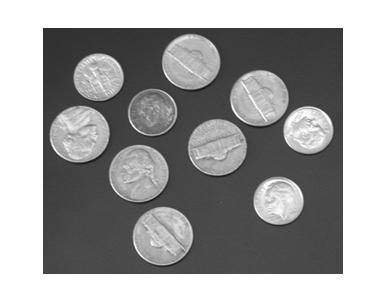
12 12 In the result of convolving a 2-D image with the Laplacian of a Gaussian, the rate of change of the convolution result as it crosses zero, which we will call the slope of the zero-crossing, can be used as a rough measure of the contrast and sharpness of the intensity changes. Intensity changes can occur at any orientation in the image. At the location of a zero-crossing contour, the slope of the convolution result is always steepest in the direction perpendicular to the contour. The gradient of a 2-D function is a vector defined at each location of the function that points in the direction of steepest increase of the function. This vector can be constructed by measuring the derivative of the function in the x and y directions. The horizontal and vertical components of the gradient vector are the derivatives in the x and y direction: grad = (dx,dy). The magnitude of this gradient vector indicates the rate of change of the function at each location. If we again let L(x,y) denote the result of convolving the image with the Laplacian of a Gaussian function, then at the location of a zerocrossing, the slope of the zero-crossing can be defined as follows: slope = # L& % ( $ x ' 2 # + L & % ( $ y ' 2 The derivatives of L(x,y) in the x and y directions can be calculated by subtracting the convolution values in adjacent locations of the convolution array. For example, in the convolution result shown on page 9, suppose we want to calculate the slope of the zero-crossing that occurs between location (29, 28) (i.e. row 29 and column 28) and location (29, 29). The location (29, 29) contains the value 231. The derivative in the x direction can be calculated by subtracting the value at location (29, 28), yielding 237, and the derivative in the y direction can be calculated by subtracting the value at location (28, 29), yielding 270. The result of the slope calculation is then 359. In practice, only the relative values of the slopes at different zero-crossings are important, so the slopes can be scaled to smaller values. The image below was first convolved with the Laplacian of a Gaussian. The zero-crossing contours were detected and the slopes of the zero-crossings were calculated as described above. Below the image, the zero-crossings are displayed with the darkness of the contour proportional to this measure of slope. Higher contrast edges in the original image, such as the outlines of the coins, give rise to darker (more steeply sloped) zero-crossing contours.

13 13