Introduction to Computer Vision. 2D Linear Systems

Size: px

Start display at page:

Download "Introduction to Computer Vision. 2D Linear Systems"

Warren Berry
5 years ago
Views:

1 Introduction to Computer Vision D Linear Systems

2 Review: Linear Systems We define a system as a unit that converts an input function into an output function Independent variable System operator or Transfer function

3 Linear Time Invariant Discrete Time Systems x c (t) x[n] y[n] y r (t) A/D LTIS (H) D/A jω jω jω Ye ( ) = He ( ) Xe ( ) Y ( jω ) = H( jω) X ( jω) r H( jω) Ω < π / T H( jω ) = 0 Ω π / T c IF The input signal is bandlimited The Nyquist condition for sampling is met The digital system is linear and time invariant THEN The overall continuous time system is equivalent to a LTIS whose frequency response is H.

4 Overview of Linear Systems Let where f i (x) is an arbitrary input in the class of all inputs {f(x)}, and g i (x) is the corresponding output. If Then the system H is called a linear system. A linear system has the properties of additivity and homogeneity. 4

5 Linear Systems The system H is called shift invariant if for all f i (x) {f(x)} and for all x 0. This means that offsetting the independent variable of the input by x 0 causes the same offset in the independent variable of the output. Hence, the input-output relationship remains the same. 5

6 Linear Systems The operator H is said to be causal, and hence the system described by H is a causal system, if there is no output before there is an input. In other words, A linear system H is said to be stable if its response to any bounded input is bounded. That is, if where K and c are constants. 6

7 Linear Systems A unit impulse function, denoted δ(a), is defined by the expression δ(a) δ(x-a) x a The response of a system to a unit impulse function is called the impulse response of the system. h(x) = H[δ(x)] 7

8 Linear Systems If H is a linear shift-invariant system, then we can find its reponse to any input signal f(x) as follows: This expression is called the convolution integral. It states that the response of a linear, fixed-parameter system is completely characterized by the convolution of the input with the system impulse response. 8

9 Linear Systems Convolution of two functions of a continuous variable is defined as f ( x)* h( x) = f( α) h( x α) dα In the discrete case f [ n]* h[ n] = f[ m] h[ n m] m= 9

10 Linear Systems In the D discrete case f [ n, n ]** h[ n, n ] = f[ m, m ] h[ n m, n m ] m = m = hn [, n] is a linear filter. 0

11 Illustration of the folding, displacement, and multiplication steps needed to perform two-dimensional convolution f(α,β) g(α,β) (a) α A B β α β (b) g(x - α,y - β) f(α,β)g(x - α,y - β) B (c) α y x β x α y Volume = f(x,y) g(x,y) β (d)

12 Matrix perspective i f c h e b g d a step c b a a b c f e d d e f i h g g h i step

13 Convolution Example h f Rotate From C. Rasmussen, U. of Delaware

14 4 Convolution Example Step f f*h h - - -

15 5 Convolution Example f f*h h - - -

16 6 Convolution Example f f*h h - - -

17 7 Convolution Example f f*h - - -

18 8 Convolution Example f f*h h - - -

19 9 Convolution Example f f*h h - - -

20 Convolution Example and so on From C. Rasmussen, U. of Delaware 0

21 Example: averaging 9 * = Integration

22 Example: edge detection 8 * = Deriving

23 Try MATLAB f=imread( saturn.tif ); figure; imshow(f); [height,width]=size(f); f=f(:height/,:width/); figure; imshow(f); [height,width=size(f); f=double(f)+0*rand(height,width); figure;imshow(uint8(f)); h=[ ; ; ; ]/6; g=conv(f,h); figure;imshow(uint8(g));

24 Gaussian Lowpass Filter 4

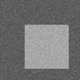
25 Gaussian Lowpass Denoising Original σ = σ = 4 5

26 Image Processing Algorithms

27 IP Algorithms Spatial domain Operations are performed in the image domain Image matrix of number Examples luminance adaptation chromatic adaptation contrast enhancement spatial filtering edge detection noise reduction Transform domain Some operators are used to project the image in another space Operations are performed in the transformed domain Fourier (DCT, FFT) Wavelet (DWT,CWT) Examples coding denoising image analysis Most of the tasks can be implemented both in the image and in the transformed domain. The choice depends on the context and the specific application. 7

28 Spatial domain processing Pixel-wise Operations involve the single pixel Operations: histogram equalization change of the colorspace addition/subtraction of images get negative of an image Applications: luminance adaptation contrast enhancement chromatic adaptation Local-wise The neighbourhood of the considered pixel is involved Any operation involving digital filters is local-wise Operations: correlation convolution filtering transformation Applications smoothing sharpening noise reduction edge detection 8

29 Pixel-wise operations Histogram Straching/shrinking, sliding Equalization

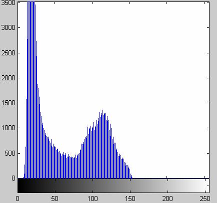
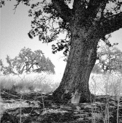
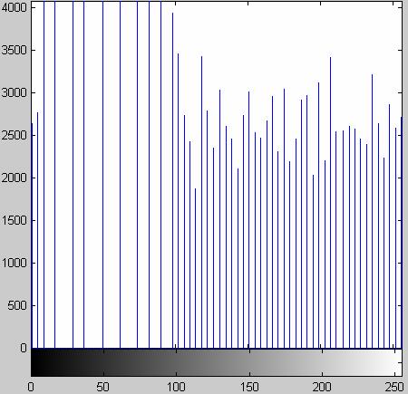
to a uniform distribution over a given number of grey levels.

30 Pixel-wise: Histogram equalization Pixel features: luminance, color, Histogram equalization: shapes the intensity histogram to approximate a specified distribution It is often used for enhancing contrast by shaping the image histogram to a uniform distribution over a given number of grey levels. The grey values are redistributed over the dynamic range to have a constant number of samples in each interval (i.e. histogram bin). Can also be applied to colormaps of color images. 0

31 Histogram equalization Can be used to compensate the distortions in the gray level distribution due to the non-linearity of a system component Gamma function = < > top top top bottom bottom bottom low height low height low height gamma=0. gamma=4

32 Histogram equalization Enhances the contrast of images by transforming the values in an intensity image so that the histogram of the output image approximately matches a specified histogram also applies to the values in the colormap of an indexed image

33 Histogram Function H=H(g) indicating the number of pixels having gray-value equal to g Non-normalized images: 0 g 55 bin-size, can be integer Normalized images: 0 g bin-size< H(l) 0 g i or 55 g A A = = max 0 N g i= Hgdg ( ) H[ g ] i area under the curve=number of pixels In the continuous case da( g) A( g) A( g +Δg) Hg ( ) = = lim dg Δg 0 Δg

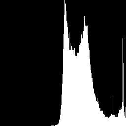
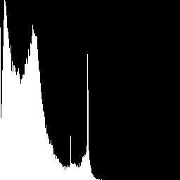
34 Example: region-based segmentation If the two regions have different graylevel distributions (histograms) then it is possible to split them by exploiting such an information A H A H 4

35 Example: region-based segmentation 5

36 Types of operations Histogram equalization contrast enhancement Histogram stratching/shrinking expansion/compression of the dynamic range Loss of resolution (the same set of pixel values are represented by a subset of graylevel values) Histogram sliding change of the mean level 6

37 H. stratching/shrinking 0 I g min stretch[ I ] = g g + g 0 0 g max g min g g g 0 max 0 min max min max min min = max I[ i, j] = maximum gray value in the original image g min I[ i, j] = minimum gray value in the original image g, g = maximum and minimum gray values in the processed image 7

38 H. original 8

39 H. shrinked 9

40 H. stratched 40

41 H. sliding 4

42 H. stratching/shrinking stratching shrinking 4

43 4

44 Linear graylevel transformations g new H b g old g H H g g 44

45 Non-linear tranformations Used to emphasize mid-range levels g new = g old + g old C (g old,max -g old ) g new g old 45

46 Common transformations g out g out g in g in g out ldg out g in Intensity slicing g in 46

47 Sigmoid transformation (soft thresholding) g out H(g in ) H(g out ) g in g in g out 47

48 Histogram transformation g f g g f g f out = ( in ) in = ( out ), non-decreasing function Hg ( ) Hg ( ), namely in out H f g f Hg ( out ) =, f' = f '[ f ( g )] g [ ( out )] out 48

49 Histogram equalization Let x be a random variable and let n i be the number of occurrences of gray level i. The probability of an occurrence of (a pixel of level) i in the image is L being the total number of gray levels in the image, n being the total number of pixels in the image, and p x being in fact the image's histogram, normalized to [0,]. Let us also define the cumulative distribution function corresponding to p x as 49

50 We would like to create a transformation of the form y = T(x) to produce a new image {y}, such that its CDF will be linearized across the value range, i.e. cdf () i = K i y The properties of the CDF allow us to perform such a transform it is defined as y = T( x) = cdf ( x) x 50

51 Pictorially p x pdf p y pdf /g max cdf g max g cdf g max g cdf x cdf y /g max g max g g max g 5

52 5

53 5

54 54

55 Neighborhood operations Correlation pattern recognition Convolution Linear filtering Edge detection Denoising

56 Correlation Correlation Measures the similarity between two signals Difference from convolution: no minus signs in the formula the signals need only to be translated f [ m, n] htemplate[ m+ k, n+ C ( m, n) = r] k r g... Application database matching result pattern 56

57 Convolution g[ m, n] = f [ m, n] hfilter[ m, n] = f [ m, n] h G( jω, jω ) = x y F( jω, x jω ) H y k, r filter ( jω, x jω ) y filter [ k m, r n] f [ m, n]:original(input)image g[ m, n]:filtered(output)image h filter [ m, n]:filter impulseresponse 57

58 Convolution and digital filtering Digital filtering consists of a convolution between the image and the impulse response of the filter, which is also referred to as convolution kernel. Warning: both the image and the filter are matrices (D). If the filter is separable, then the D convolution can be implemented as a cascade of two D convolutions Filter types FIR (Finite Impulse Response) IIR (Infinite IR) 58

59 Ideal low-pass digital filter H(Ω) -π -Ω c Ω c Ω N π Ω Digital LP filter (discrete time) The boundary between the pass-band and the stop-band is sharp The spectrum is periodic The repetitions are located at integer multiples of π The low-pass filtered signal is still a digital signal, but with a different frequency content The impulse response h[n] in the signal domain is discrete time and corresponds to the sinc[] function Reconstruction LP filter (continuous time) The boundary between the pass-band and the stop-band is sharp The spectrum consists of one repetition only The low-pass filtered signal is a continuous time signal, that might have a different frequency content The impulse response h(t) in the signal domain is continuous time and corresponds to the sinc() function 59

60 Digital LP filtering H(Ω) -π -Ω c Ω c π F(Ω) low-pass filtered (digital) signal F(Ω) H(Ω) 60

61 Low-pass LP and HP filtering High-pass H LP (Ω) H HP (Ω) h LP [n] h HP [n] n n averaging 6

62 Example: Chebyshev LP 6

63 Example: Chebyshev HP 6

64 Example: Chebyshev Impulse Response 64

65 Example: Chebyshev Step Response 65

66 Example: filtered signal The transfer function (or, equivalently, the impulse response) of the filter determines the characteristics of the resulting signal 66

67 Switching to images qui Images are D digital signals (matrices) filters are matrices Low-pass averaging (interpolation) smoothing High-pass differentiation emphasize image details like lines, and, more in general, sharp variations of the luminance Band-pass: same as high pass but selecting a predefined range of spatial frequencies Splitting low-pass and high-pass image features is the ground of multiresolution. It is advantageous for many tasks like contour extraction (edge detection), image compression, feature extraction for pattern recognition, image denoising etc. 67

68 68 D filters Low-pass High-pass = 9 h lowpass = 8 h highpass

69 Filtering in image domain Filtering in image domain is performed by convolving the image with the filter kernel. This operation can be though of as a pixel-by-pixel product of the image with a moving kernel, followed by the sum of the pixel-wise output. 69

70 Low-pass filtering: example f[m,n] h lowpass [m,n] g[m,n] x = 70

71 Averaging h lp =/5 7

Gaussian h lp = 0.000 0.0 0.09 0.0 0.000 0.0 0.0596 0.098 0.0596 0.0 0.09 0.098 0.6 0.098 0.09 0.0 0.0596 0.098 0.0596 0.0 0.000 0.0 0.09 0.0 0.000 7

72 Gaussian h lp =

Log 0.09 0.0460 0.0499 0.0460 0.09 0.0460 0.006-0.

0460 0.006-0.09 0.006 0.0460 0.09 0.0460 0.0499 0.

73 Log

74 Asymmetric LP h lp =/

75 Asymmetric HP h lp =

76 Sharpening Goal: improve image quality Solutions increase relative importance of details, by increasing the relative weight of high frequencies components Increase a subset of high frequencies (non symmetric HP) High-boost filter Laplacian gradient The original image is assumed to be available 76

77 Sharpening Filters To highlight fine detail or to enhance blurred details Averaging filters smooth out noise but also blur details Sharpening filters enhance details May also create artifacts (amplify noise) Background: Derivative is higher when changes are abrupt Categories of sharpening filters: Basic highpass spatial filtering High-boost filtering 77

78 Sharpening Original image HP Normalization + Sharpened image Normalization The normalization step subtracts the mean and scales the amplitude of the resulting image by dividing it for the dynamic range (graylevel values are now in the range 0-55) For the sharpening to be visible, the sharpened and original images must then be displayed using the same set of graylevel values 78

79 Basic Highpass Spatial Filtering The filter should have positive coefficients near the center and negative in the outer periphery: Laplacian mask Other Laplacian masks (normalization factor is missing) 79

80 Basic Highpass Spatial Filtering The sum of the coefficients is 0, indicating that when the filter is passing over regions of almost stable gray levels, the output of the mask is 0 or very small. The output is high when the center value differ from the periphery. The output image does not look like the original one. The output image depicts all the fine details Some scaling and/or clipping is involved (to compensate for possible negative gray levels after filtering). 80

81 8

82 High boost Examples 8

83 High-boost Filtering Highpass filtered image = Original lowpass filtered image If A is an amplification factor, then: High-boost = A original lowpass = (A-) original + original lowpass = (A-) original + highpass Unsharp masking (if A=) 8

84 Unsharp Masking and Sharpening operation Signal Low- pass () () High-pass () = () - () (A-) () + () 84

85 High-boost Filtering A= : standard highpass result A > : the high-boost image looks more like the original with a degree of edge enhancement, depending on the value of A. A > Unsharp masking w=9a-, A 85

86 86

87 Unsharp masking 87

88 Sharpening: asymmetric HP 88

89 Sharpening: the importance of phase 89

90 Sharpening: the importance of phase 90

91 Sharpening: the importance of phase 9

92 Sharpening: the importance of phase 9

93 Back to the natural image 9

Image Enhancement in the frequency domain. GZ Chapter 4

Image Enhancement in the frequency domain GZ Chapter 4 Contents In this lecture we will look at image enhancement in the frequency domain The Fourier series & the Fourier transform Image Processing in