Image Processing. Waleed A. Yousef Faculty of Computers and Information, Helwan University. April 3, 2010

Transcription

1 Image Processing Waleed A. Yousef Faculty of Computers and Information, Helwan University. April 3, 2010

2

3 Ch3. Image Enhancement in the Spatial Domain

4

5 Note that T (m) = 0.5 E. The general law of contrast stretching is T (r) = (m/r) E.

6

7

8 PLEASE, take care of storage classes (image types): if f = then mat2gray(f) will scale the whole range [.5, 1.5] to produce However, im2uint8(f) will truncate any thing outside [0, 1] to produce

9 Therefore, to convert f to an 8-bit image we have to scale it right to the range [0, 1] then convert it to an image. E.g., im2uint8(mat2gray(c*log(1+f)))

10

11

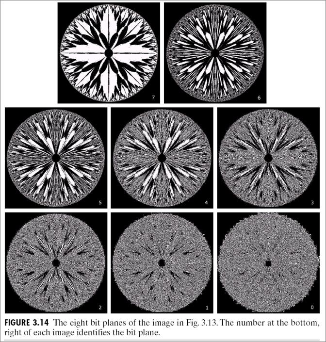
12

13

14

15 When we look at this image we feel that we need to darken the dark and whiten the white; which means stretch the contrast. So, it includes two power-law transformations with values of γ below and above one! (see figure 3.10a)

16

17

18

19

20 All of these images are binary. A pixel has one or zero depending on the value of bit-plane of this pixel. A bit plane can be easily calculated by dividing by 2 b, where b is the required bit level. In C, this can be done faster by shifting. (Try both) Advanced Homework: Write a C program that does bit-shift and link it to Matlab to extract the right bit-plane.

21

22 s = r 0 p r (x) dx Histogram Equalization s = T (r), s 0 p s (x) dx = r 0 p r (x) dx If p s is requied to be uniform, then

23 for any arbitrary desired p s G s (s) = r 0 p r (x) dx, s = G 1 ( r s 0 p r (x) dx )

24

25

26 Histogram Matching

27

28

29

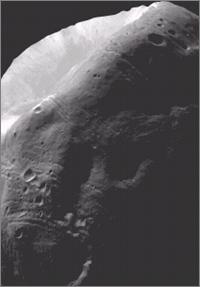
30 Try enhancing this image using piece-wise transformation that tries to whiten the dark and keep the rest as is, or a power-law transformation with γ < 1; what is the difference? Let s try understanding the image first through this code, and run it in Matlab. figure ; imshow ( imadjust ( f, [ ], [ ],. 8 ) ) ; title ( power transformation with \gamma =. 8 ) ; Matlab Code 1: clc ; f=imread ( Fig ( a ). jpg ) ; whos f ; figure ; imshow ( f ) ; title ( o r i g i n a l image ) ; % D o e s t h e b a c k g r o u n d ( l e f t u p e r ) d a r k e r t h a n t h e r i g h l o w e r p a r t o f t h e % m o o n? L e t s s e e : f ( 1 : 1 0, 1 : 1 0 ) f (end 9:end, end 9:end) % N o, t h e r i g h t l o w e r i s d a r k e r! T a k e c a r e w h i l e p r o c e s s i n g. % L e t s s e e p o w e r t r a n s f o r m a t i o n :

31 figure ; imshow ( imadjust ( f, [ ], [ ],. 6 ) ) ; title ( power transformation with \gamma =. 6 ) ; figure ; imshow ( imadjust ( f, [ ], [ ],. 4 ) ) ; title ( power transformation with \gamma =. 4 ) ; % T o h o w l o n g s h o u l d I k e e p d e c r e a s i n g g a m m a? l e t s s e e w h e t h e r t h e i m a g e % i t s e l f i s t o o d a r k ; t h i s i s b y m a r k i n g t h e r e g i o n s o f 0 g r a y l e v e l a s % w h i t e. tmp=f ; tmp( find (tmp==0)) =255; figure ; imshow (tmp) ; title ( p i x e l s with zero gray l e v e l are marked as white ) ; % T h e r e f o r e, s c a l i n g w i l l k e e p t h e s e p i x e l s u n c h a n g e d!!

32 Global Histogram Statistics m = L 1 k=0 = L 1 k=0 r k p (r k ) n k r k n L 1 = 1 n = 1 MN k=0 r k n k M N i=1 j=1 f (i, j) So, averaging over pixels or using histogram is of course the same. statistics. The same is for other σ 2 = L 1 k=0 = 1 MN (r k m) 2 p (r k ) M N i=1 j=1 Local Histogram Statisticsge for a regoin S xy m Sxy = k = 1 S xy r k p (r k ) (f (i, j) m)2 f (i, j), (i,j) S xy

33 where S xy is the number of pixels in the region S xy. The figure is not available online, but we can easily make our code and image: Matlab Code 2: f=uint8 ( zeros (100:100) ) ; f ( 4 0 : 6 0, 40:60) =10; figure ; imshow ( f ) ; tmp=uint8 ( zeros ( size ( f, 1), size ( f, 2) ) ) ; % T a k e c a r e o f t h e u i n t 8 ; w i t h o u t i t t m p w i l l b e d o u b l e a n d a n y p i x e l

34 tmp=uint8 ( zeros ( size ( f, 1), size ( f, 2) ) ) ; l a r g e r t h a n o n e w i l l b e t r e a t e d a s 1 w=3; % t h e w i n d o w w i d t h i s 2 w + 1 for i=1+w: size ( f, 1) w for j=1+w: size ( f, 2) w win=h i s t e q ( f ( i w: i+w, j w: j+w) ) ; tmp( i, j )=win (w+1, w+1) ; % t h e m i d d l e p i x e l end; end; figure ; imshow (tmp) ; Now, let s see how local histogram equalization affects the photo of the moon: Matlab Code 3: f=imread ( Fig ( a ). jpg ) ; f=f ( 1 : 4 : end, 1 : 4 : end) ; % t o s p e e d u p e x e c u t i o n figure ; imshow ( f ) ;

35 However, with width 31(= ) it enhances local details but with leaving the black areas unchanged. w=25; % t h e w i n d o w w i d t h i s 2 w + 1 for i=1+w: size ( f, 1) w for j=1+w: size ( f, 2) w win=h i s t e q ( f ( i w: i+w, j w: j+w) ) ; tmp( i, j )=win (w+1, w+1) ; % t h e m i d d l e p i x e l end; end; figure ; imshow (tmp) ; title (w) ; Using a window of width 7(= ) gives this un-useful image:

36

37

38

39

40

41

42 Image Averaging g (x, y) = f (x, y) + η (x, y), where f (x, y) is the original image and η (x, y) is an additive noise, usually with zero mean. K g (x, y) = 1 g i (x, y), K k=1 E g (x, y) = f (x, y) Var g (x, y) = 1 K Var η (x, y), This is assuming that the noise η has zero mean and uncorrelated.

43

44

45 Basics of Spatial Filtering

46

47 The general form of a spatial filter is:

48

49

50 Image processed by averaging mask, followed by thresholding the gray level at 25%.

51 Median filter is effective in removing Salt-and-pepper noise. For example, in a 3 3 neighborhood, the median is the 5th largest value.

52 Sharpening Spatial Filters Since the idea of blurring involves integration (summation), we can anticipate that sharpening should involve differentiation. How should it be defined over a discrete space? Discrete derivative should possess: 2 f = f (x + 1) + f (x 1) 2f (x) x2 zero in flat segments. non-zero at the onset of a gray-level step or ramp. non-zero along ramps. which is also consistent with 2nd derivative should possess: zero in flat segments. f x f x = lim x 0 = f (x + 1) f (x), f (x + x) f (x) x non-zero at the onset and end of a gray-level step or ramp. zero along ramps with constant slope

53 Prove that these definitions of derivatives possess the desired properties. 1. First-order derivaties genrally produce thicker edges in an image. The definition of the second derivative should comply with applying the first derivative on the first derivative; i.e., 2 f x 2 x = f x x = (f (x + 1) f (x)) x = x f (x + 1) x f (x) = [f ((x + 1) + 1) f (x + 1)] [f (x + 1) f (x)] = f (x + 2) + f (x) 2f (x + 1) = 2 f x 2 (using book def.!) x+1 Said differently, 2 f x 2 book x = f x x x 1 It would be, mathematically, more consistent to use the other def. The following properties are observable from the following figure:

54 2. Second-order derivatives have a stronger response to fine detail, such as thin lines and isolated points. First-order derivatives are good for extracting edges. 3. First-order derivatives generally have a stronger response to a gray-level seop. 4. Second-order derivatives produce a double response at step changes in gray level. In general: Second-order derivatives are good in enhancing fine details.

55

56 Use of Second Derivatives for Enhancement (The Laplacian) This can be implemented using the follwing mask, with the ability to add the diagonal componenets as well. This is a linear operator and isotropic (invariant to rotation). 2 f = 2 f x f y 2. For digital image, we can define it as 2 f = [f (x + 1, y) + f (x 1, y) 2f (x, y)] + [f (x, y + 1) + f (x, y 1) 2f (x, y)] = f (x + 1, y) + f (x 1, y) + f (x, y + 1) + f (x, y 1) 4f (x, y).

57 The Laplacian will produce an image of grayish edges and discontinuties with featureless background. So, if superimposed on the original image it will enhance the fine details at which the

58 second derivatives produce this grayish edges: g (x, y) = f (x, y) 2 f g (x, y) = f (x, y) + 2 f for negative mask center, for positive mask center

59

60

61

62

63

64

65

66

67 Bibliography