Colorado School of Mines Image and Multidimensional Signal Processing

Transcription

1 Image and Multidimensional Signal Processing Professor William Hoff Department of Electrical Engineering and Computer Science

2 Spatial Filtering

3 Main idea Spatial filtering Define a neighborhood of a pixel Define an operation on pixels in the neighborhood Output pixel value = result of the operation Topics Linear filtering Correlation, convolution Normalized cross correlation Important examples Smoothing filters (box average, Gaussian) Sharpening filters (Laplacian, Sobel) Non-linear filters Order-statistics filters (primarily median filter) 3

4 Linear Spatial Filtering Create a filter or mask w, size m x n Apply to image f, size M x N Compute the sum of products of mask coefficients with corresponding pixels under mask Slide mask over image, apply at each point m/ n/ g( x, y) w( s, t) f ( x s, y t) sm/ tn/ w( x, y) f ( x, y) Also called crosscorrelation It is a linear operation w( x, y) a f ( x, y) a w( x, y) f ( x, y) w( x, y) f ( x, y) g( x, y) w( x, y) f ( x, y) w( x, y) g( x, y) 4

5 / / / / ), ( ), ( ), ( m m s n n t t y s x f t s w y x g 5

6 Example 3x3 averaging ( box ) filters Do manual calculation on a corner f ( x, y) g( x, y) w( x, y) f ( x, y) : : : : : : :.. 6

7 Example 3x3 averaging filters Manual calculation on corner 7

8 Matlab Examples clear all close all % Synthetic image of a white square I = zeros(00,00); I(50:150, 50:150) = 1; imshow(i,[]); % Apply 3x3 box filter w = [ 1 1 1; 1 1 1; 1 1 1]/9; I = imfilter(i, w); imtool(i,[]); fspecial useful to create filters imfilter does cross correlation % Apply 15x15 box filter w = fspecial('average', [15 15]); I3 = imfilter(i, w); imtool(i3,[]); % Show that averaging reduces noise I = I + randn(00,00)*0.5; imshow(i,[]); w = fspecial('average', [5 5]); I4 = imfilter(i, w); figure, imshow(i4,[]); 8

9 Sharpening Spatial Filters First Derivative First derivative f ( x, y) f ( x, y) f ( x, y) lim x 0 In discrete form (can also do central difference) f ( x, y) f ( x 1, y) f ( x, y) f f ( x 1) f ( x 1) / x x As a filter Sobel operators combine smoothing with derivative dx filter dy filter

10 w( x, y) Example f ( x, y) g( x, y) w( x, y) f ( x, y)

11 w( x, y) Example f ( x, y) g( x, y) w( x, y) f ( x, y)

12 Gradient Compute gradient components using first derivative operators f f f x y Gradient magnitude indicates the location of edges in the image f f x f y 1/ Gradient direction shows direction of edge We can use the Sobel operators for df/dx, df/dy 1 f y tan f x 1

13 Matlab example clear all close all I = imread('moon.tif'); imshow(i,[]); % Create Sobel filters hy = [ % can also do hy = fspecial('sobel'); ; 0 0 0; ]; hx = hy'; Ix = imfilter(i, hx); Iy = imfilter(i, hy); figure; subplot(1,,1), imshow(ix,[]); subplot(1,,), imshow(iy,[]); Note - the result is not quite correct We should first convert the input image to type double before applying imfilter (why?) 13

14 Matlab example (continued) % Compute gradient magnitude (note the use of ".") Ig = (Ix.^ + Iy.^).^ 0.5; figure, imshow(ig, []); >> help atan atan Four quadrant inverse tangent. atan(y,x) is the four quadrant arctangent of the real parts of the elements of X and Y. -pi <= atan(y,x) <= pi. See also atan. Reference page in Help browser doc atan % Compute gradient direction Iang = atan(iy,ix); figure, imshow(iang, []); % Only display angles where gradient magnitude is large Mask = (Ig > 100); figure, imshow(double(mask).* Iang, []); colormap jet 14

15 Sharpening Spatial Filters nd derivative Second derivative f x y x x x (, ) f ( x, y) f ( x 1, y) f ( x, y) f ( x 1, y) As a filter Two dimensional the Laplacian As a filter f f f x y x x =

16 High Boost Filtering We combine original image with results of Laplacian result is the original image with enhanced detail g( x, y) f ( x, y) f Also called unsharp masking In general g( x, y) Af ( x, y) f ( x, y) 16

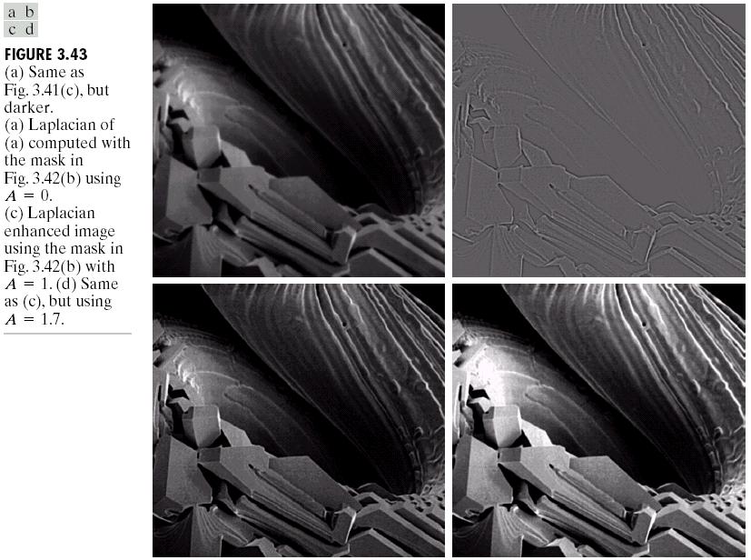
17 17

18 Vector representation of correlation Correlation is a sum of products of corresponding terms We can think of correlation as a dot product of vectors w and f c w f w f w f mn k1 1 1 wf k k m/ n/ c( x, y) w( s, t) f ( x s, y t) sm/ tn/ w( x, y) f ( x, y) T wf mn mn If images w and f are similar, their vectors are aligned 18

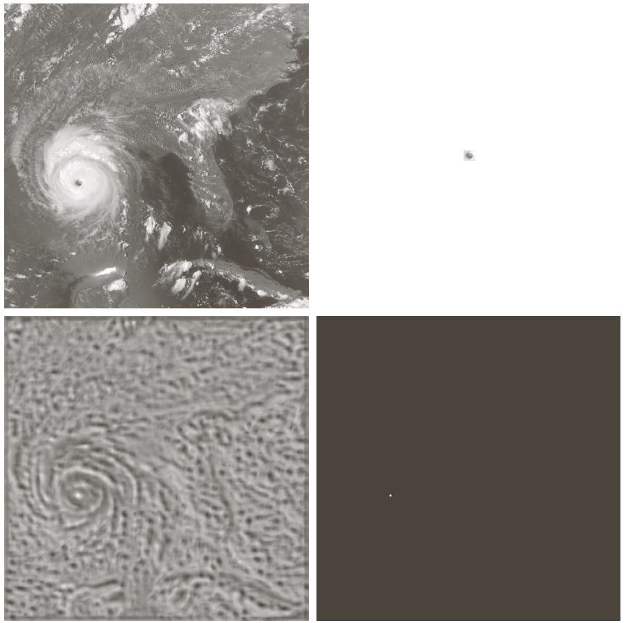
19 Correlation can do matching Let w(x,y) be a template subimage Try to find an instance of w in image f(x,y) The correlation score c(x,y) is high where w matches f m/ n/ c( x, y) w( s, t) f ( x s, y t) sm/ tn/ w( x, y) f ( x, y) 19

20 0

21 Template Matching (continued) Since f is not constant everywhere, we need to normalize c wf T w f where w w 1 w w 3 w N The result is between 0..1 (for positive valued images) We can get better precision by subtracting off means c( x, y) st, s, t s, t This result is between [ w( s, t) w][ f ( x s, y t) f ] [ w( s, t) w] [ f ( x s, y t) f ] 1/ This is the normalized correlation coefficient 1

22 Normalized Cross-correlation Normalized cross-correlation (values range from ) c( x, y) where st, s, t s, t w(s,t) is a subimage, size mxn f(x,y) is a large image, size MxN sums are taken over s=1..m, t=1..n [ w( s, t) w][ f ( x s, y t) f ( x, y)] [ w( s, t) w] [ f ( x s, y t) f ( x, y)] f ( x, y) is the local mean of f, in a mxn neighborhood around (x,y) 1/ 1 f ( x, y) f ( x s, y t) mn st, See pg. 870 in the Gonzalez & Woods textbook w(s,t) Size mxn f(x,y) c(x,y) Correlation scores Size MxN Size MxN

23 Matlab Example Crop a small subimage from left image, find its match in the right image I1 = imread('test000.jpg'); T = imcrop(i1, [66, 13, 86, 33]); I = imread('test01.jpg'); C = normxcorr(t, I); % The scores are in an image that is slightly bigger than the original % image... it is expanded by half the size of the template in all % directions. So we will crop out the center portion. Csub = imcrop(c, [(size(t,)-1)/+1 (size(t,1)-1)/+1 size(i,)-1 size(i,1)-1]); cmax = max(csub(:)); [y x] = find(csub==cmax); 3

24 Doing cross correlation in Matlab without normxcorr The easiest way is to implement the equation directly, using for loops You scan through the image... at every pixel (x,y): Extract the subimage fs(x,y) from the image f surrounding x,y Subtract off the local image mean value at (x,y) Compute the sum of the product of (fs-fmean) and (w-mean(w); this is the numerator The denominator can be similarly computed Dividing the two gives you the value of the normalized cross correlation at pixel (x,y) in the ouput Note - there are faster ways to do this, using Matlab s ability to operate on whole matrices 4

25 Doing cross correlation in Matlab without normxcorr (continued) Numerator where N [ w( s, t) w][ f ( x s, y t) f ( x, y)] st, w is the mean of all pixels in w; it can be computed once. It is a scalar. f ( x, y) is the local mean of pixels in f, in a mxn window centered at (x,y). This can be represented as an image of size MxN. Then st, [ w( s, t) w][ f ( x s, y t) f ( x, y)] [ w( s, t) w] f ( x s, y t) f ( x, y) [ w( s, t) w] s, t s, t The first term is the correlation of (w-wmean) and f. The second term is zero because [ w( s, t) w] w( s, t) w mnw mnw 0 So in Matlab: N = imfilter(f,w-mean(w)); s, t s, t s, t 5

26 Doing cross correlation in Matlab without normxcorr (continued) Denominator D [ w( s, t) w] [ f ( x s, y t) f ( x, y)] s, t s, t In Matlab, you can compute fmean at every pixel by filtering with a mxn rectangle of 1 s (and dividing by mxn): [m n] = size(w); fmean = imfilter(f, ones(m,n))/(m*n); The first term is a scalar, and can be computed once. We rewrite the second term: st, [ f ( x s, y t) f ( x, y)] f ( x s, y t) f ( x, y) f ( x s, y t) f ( x, y) s, t s, t s, t f ( x s, y t) ( mn) f ( x, y) ( mn) f ( x, y) st, f ( x s, y t) ( mn) f ( x, y) st, 1/ This can be computed by filtering again with a mxn rectangle of 1 s; i.e., imfilter(f.^, ones(m,n)) 6

27 Correlation and Convolution Correlation m/ n/ g( x, y) w( s, t) f ( x s, y t) sm/ tn/ w( x, y) f ( x, y) Convolution m/ n/ g( x, y) w( s, t) f ( x s, y t) sm/ tn/ w( x, y) f ( x, y) Note that Convolution is very similar to correlation, except that we flip one of the functions Also a linear operation m/ n/ m/ n/ w( s, t) f ( x s, y t) w( s, t) f ( x s, y t) sm/ tn/ sm/ tn/ So to implement convolution we can reflect w(x,y) and then do correlation 7

28 1D Examples Figure 3.9 8

29 1D Examples 9

30 D Examples 30

31 D Examples 31

32 Properties Convolution is Commutative f * g = g * f Associative f * (g * h) = (f * g) * h Distributive f * (g + h) = f * g + f * h Correlation is distributive but not commutative or associative Convolution of a filter h(x,y) with an impulse d(x,y) yields h(x,y) 3

33 Gaussian an important smoothing filter 1D Notes: h( x) 1 x e is the standard deviation Values should sum to 1 Mask size should be at least ±3 D x y 1 h( x, y) e

34 Convolving with two Gaussians You can convolve a function with a Gaussian, then convolve again with a Gaussian. The effect is the same as convolving with a single, larger Gaussian Why? Since convolution is associative g g f g g f 1 1 and if then x x 1 1 1, 1 g e g e 1 1 g1g e 1 x 1 i.e., it is a Gaussian with standard deviation new 1 34

35 Proof You can prove this from the definition of convolution f g f ( t) g( t x) dt And use the idea that t x t x/ e e e e e t t txx x / where the last term does not depend on t and the first one is just another Gaussian, but centered around a different point. 35

36 Interesting fact If you repeatedly convolve an image N times with any filter, the effect (for large N) is that of convolving with a Gaussian This comes from the Central Limit Theorem: The sum of N mutually independent random variables with zero means and finite variances tends toward the normal probability distribution And the fact that the pdf of the sum of two independent random variables is the convolution of their pdf s

37 Separable kernels (filter masks) If a D correlation (or convolution) kernel can be separated into two 1D kernels, the operation is much faster If then h ( x, y) h1 ( x) h ( y) h( x, y) f ( x, y) h ( x) h ( y) f ( x, y) 1 Namely, do a 1D correlation with h (y) along the individual columns of the input image, then do a 1D correlation with h 1 (x) along the rows of the result from the previous step If h(x,y) is nxn, and f(x,y) is NxN Cost of a D correlation? Cost of two 1D correlations? 37

38 Separable kernels (filter masks) If a D correlation (or convolution) kernel can be separated into two 1D kernels, the operation is much faster If then h( x, y) h1 ( x) h ( y) h( x, y) f ( x, y) h ( x) h ( y) f ( x, y) 1 Prove this (HW) Namely, do a 1D correlation with h (y) along the individual columns of the input image, then do a 1D correlation with h 1 (x) along the rows of the result from the previous step If h(x,y) is nxn, and f(x,y) is NxN Cost of a D correlation? Cost of two 1D correlations? 38

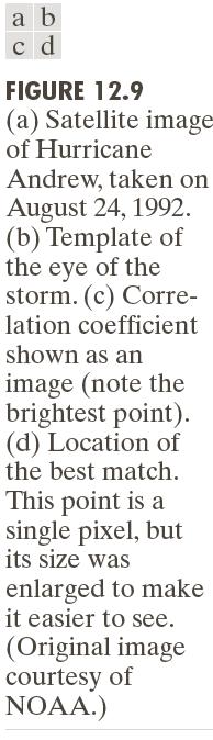
39 Nonlinear Filters Median filter - a non-linear smoothing filter Steps: Order (sort) pixel values within neighborhood Replace center with some value based on the ordering (i.e., median) Advantages Especially good for reducing impulse, or shot-and-pepper noise Doesn t blur sharp edges in the image 1 1 Matlab functions medfilt1, medfilt, ordfilt D noisy step edge median filtered, filter width=7 39

40 Example on ramp edge f( x) x x 1: 4,6 :10 0 x

41 Example on ramp edge f( x) x x 1: 4,6 :10 0 x

42 4

43 Read image eight.tif Add noise: imnoise Examples - Matlab Compare imfilter, medfilt clear all close all I = imread('eight.tif'); imshow(i,[]); Inoisy = imnoise(i, 'salt & pepper', 0.05); imtool(inoisy,[]); I1 = imfilter(inoisy, fspecial('average')); imshow(i1, []); I = medfilt(inoisy); imshow(i, []); 43

44 Summary A spatial filter operates on a neighborhood of a pixel. The output pixel value is the result of the operation. A linear spatial filter performs a sum of products of the neighborhood values with the corresponding filter values. The median filter is an example of a non-linear filter. Filters can be used for smoothing and sharpening. 44

45 Questions Is the D Gaussian filter separable? Why or why not? What is the difference between convolution and correlation? Why might the median filter be preferable for some situations? 45