Lecture 8: Interest Point Detection. Saad J Bedros

Transcription

1 #1 Lecture 8: Interest Point Detection Saad J Bedros sbedros@umn.edu

2 Last Lecture : Edge Detection Preprocessing of image is desired to eliminate or at least minimize noise effects There is always tradeoff between sensitivity and accuracy in edge detection The parameters that we can set for edge detection and labeling include the size of the edge detection mask and the value of the threshold A larger mask or a higher gray level threshold will tend to reduce noise effects, but may result in a loss of valid edge points #2

3 Example original image (Lena)

4 Compute Gradients X-Derivative of Gaussian Y-Derivative of Gaussian Gradient Magnitude

5 Get Orientation at Each Pixel Threshold at minimum level Get orientation theta = atan2(gy, gx)

6 #6

7 Edge Thinning: Non-maximum suppression for each orientation At q, we have a maximum if the value is larger than those at both p and at r. Interpolate to get these values.

8 Today s Lecture Goal: Find features between multiple images taken from different position or time to be robustly matched Approaches: Patch/Template Matching Interest Point Detection

9 Applications Comparison Between 2 or more images Image alignment Image Stitching 3D reconstruction Object recognition ( matching ) Indexing and database retrieval Object tracking Robot navigation

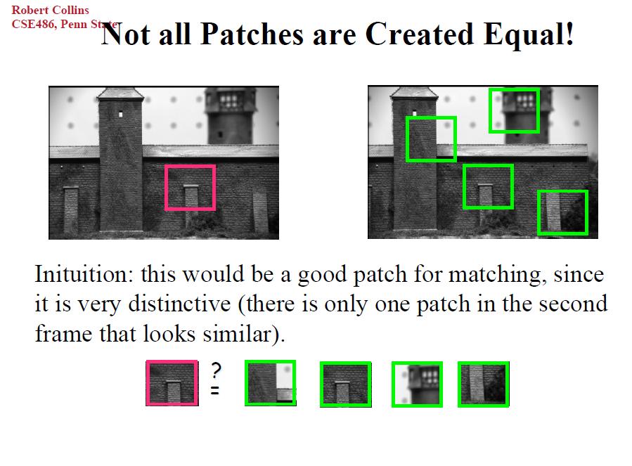
10 What points would you choose? Known as: Template Matching Method, with option to use correlation as a metric

11 Correlation #11

12 Correlation #12 Use Cross Correlation to find the template in an image Maximum indicate high similarity

13 Template/Patch Matching Options What do we do for different scales of the patch? Compute multiple Templates at different sizes Match for different scales of the template What can we do to identify the shape of the pattern at different mean brightness levels Remove the mean of the template Example in 1D

14

15 We need more robust feature descriptors for matching!!!!!

16 Interest Points Local features associated with a significant change of an image property of several properties simultaneously (e.g., intensity, color, texture).

17 Why Extract Interest Points? Corresponding points (or features) between images enable the estimation of parameters describing geometric transforms between the images.

18 What if we don t know the correspondences?? ( ) ( ) feature descriptor Need to compare feature descriptors of local patches surrounding interest points =? feature descriptor

19 Properties of good features Local: features are local, robust to occlusion and clutter (no prior segmentation!). Accurate: precise localization. Invariant / Covariant Robust: noise, blur, compression, etc. do not have a big impact on the feature. Repeatable Distinctive: individual features can be matched to a large database of objects. Efficient: close to real-time performance.

20 Invariant / Covariant A function f( ) is invariant under some transformation T( ) if its value does change when the transformation is applied to its argument: if f(x) = y then f(t(x))=y A function f( ) is covariant when it commutes with the transformation T( ): if f(x) = y then f(t(x))=t(f(x))=t(y)

21 Invariance Features should be detected despite geometric or photometric changes in the image. Given two transformed versions of the same image, features should be detected in corresponding locations.

22 Example: Panorama Stitching How do we combine these two images?

23 Panorama stitching (cont d) Step 1: extract features Step 2: match features

24 Panorama stitching (cont d) Step 1: extract features Step 2: match features Step 3: align images

25 What features should we use? Use features with gradients in at least two (significantly) different orientations patches? Corners?

26 What features should we use? (cont d) (auto-correlation)

27 Corners vs Edges #27

28 Corners in Images #28

29 The Aperture Problem #29

30 Corner Detection #30

31 Corner Detection-Basic Idea #31

32 Corner Detector: Basic Idea flat region: no change in all directions edge : no change along the edge direction corner : significant change in all directions

33 Corner Detection Using Intensity: Basic Idea Image gradient has two or more dominant directions near a corner. Shifting a window in any direction should give a large change in intensity. flat region: no change in all directions edge : no change along the edge direction corner : significant change in all directions

34 Corner Detection Using Edge Detection? Edge detectors are not stable at corners. Gradient is ambiguous at corner tip. Discontinuity of gradient direction near corner.

35 Corner Types Example of L-junction, Y-junction, T-junction, Arrow-junction, and X-junction corner types

36 Mains Steps in Corner Detection 1. For each pixel in the input image, the corner operator is applied to obtain a cornerness measure for this pixel. 2. Threshold cornerness map to eliminate weak corners. 3. Apply non-maximal suppression to eliminate points whose cornerness measure is not larger than the cornerness values of all points within a certain distance.

37 Mains Steps in Corner Detection (cont d)

38 Moravec Detector (1977) Measure intensity variation at (x,y) by shifting a small window (3x3 or 5x5) by one pixel in each of the eight principle directions (horizontally, vertically, and four diagonals).

39 Moravec Detector (1977) Calculate intensity variation by taking the sum of squares of intensity differences of corresponding pixels in these two windows. 8 directions x, y in {-1,0,1} S W (-1,-1), S W (-1,0),...S W (1,1)

40 Moravec Detector (cont d) The cornerness of a pixel is the minimum intensity variation found over the eight shift directions: Cornerness(x,y) = min{s W (-1,-1), S W (-1,0),...S W (1,1)} Cornerness Map (normalized) Note response to isolated points!

41 Moravec Detector (cont d) Use Non-maximal suppression will yield the final corners. Process of Zero out all pixels that are not the maximum along the direction of the gradient (look at 1 pixel on each side)

42 Moravec Detector (cont d) Does a reasonable job in finding the majority of true corners. Edge points not in one of the eight principle directions will be assigned a relatively large cornerness value.

43 Moravec Detector (cont d) The response is anisotropic (directionally sensitive) as the intensity variation is only calculated at a discrete set of shifts (i.e., not rotationally invariant)

44 Corner Detection: Mathematics Change in appearance of window w(x,y) for the shift [u,v]: xy, 2 Euv (, ) wxy (, ) I( x u, y v) I( x, y) I(x, y) E(u, v) E(3,2) w(x, y)

45 Corner Detection: Mathematics Change in appearance of window w(x,y) for the shift [u,v]: xy, 2 Euv (, ) wxy (, ) I( x u, y v) I( x, y) I(x, y) E(u, v) E(0,0) w(x, y)

46 Harris Detector: Mathematics Change of intensity for the shift [u,v]: xy, 2 Euv (, ) wxy (, ) I( x u, y v) I( x, y) Window function Shifted intensity Intensity Window function w(x,y) = or 1 in window, 0 outside Gaussian

47 Harris Detector #47 Improves the Moravec operator by avoiding the use of discrete directions and discrete shifts. Uses a Gaussian window instead of a square window.

48 Harris Detector (cont d) Using first-order Taylor approximation: Reminder: Taylor expansion ( n) f ( a) f ( a) 2 f ( a) n n 1 f( x) f( a) ( x a) ( x a) ( x a) O( x ) 1! 2! n!

49 Since Harris Detector (cont d)

50 Harris Detector (cont d) A W (x,y)= f ( xi, yi) ( ) x 2 f ( xi, yi) ( ) y 2 2 x 2 matrix (auto-correlation or 2 nd order moment matrix)

51 Harris Detector General case use window function: 2 S ( x, y) w( x, y ) f( x, y ) f( x x, y y) W i i i i i i x, y i i default window function w(x,y) : 1 in window, 0 outside A W 2 wxy (, ) fx wxy (, ) fx fy 2 xy, xy, fx fx f y w( x, y) 2 2 xy, fx fy fy wxy (, ) fx fy wxy (, ) f y xy, xy,

52 Harris Detector (cont d) Harris uses a Gaussian window: w(x,y)=g(x,y,σ I ) where σ I is called the integration scale window function w(x,y) : Gaussian A W 2 wxy (, ) fx wxy (, ) fx fy 2 xy, xy, fx fx f y w( x, y) 2 2 xy, fx fy fy wxy (, ) fx fy wxy (, ) f y xy, xy,

53 Harris Detector A W 2 fx fx f y 2 xy, fx fy fy Describes the gradient distribution (i.e., local structure) inside window! Does not depend on x, y

54 Harris Detector (cont d) 0 AW R R Since M is symmetric, we have: We can visualize A W as an ellipse with axis lengths determined by the eigenvalues and orientation determined by R Ellipse equation: x [ x y] AW const y direction of the fastest change (λ min ) -1/2 (λ max ) -1/2 direction of the slowest change

55 Harris Corner Detector (cont d) The eigenvectors of A W encode direction of intensity change. v 1 The eigenvalues of A W encode strength of intensity change. v 2

56 Harris Detector (cont d) Eigenvectors encode edge direction Eigenvalues encode edge strength direction of the fastest change (λ min ) -1/2 (λ max ) -1/2 direction of the slowest change

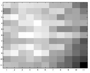
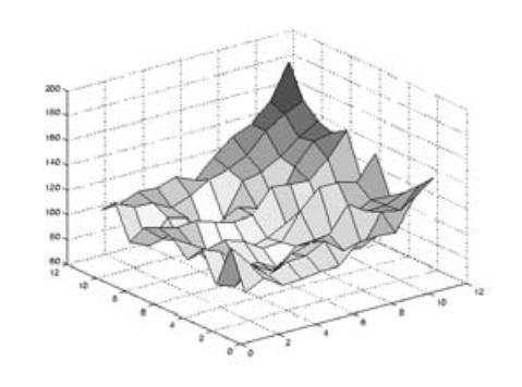
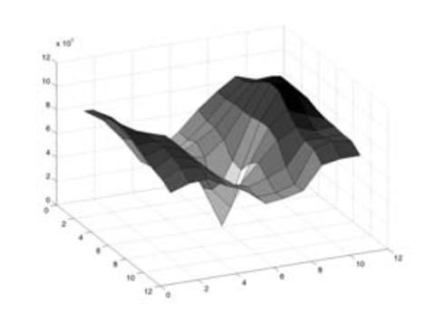
57 Distribution of fx and fy

58 Distribution of f x and f y (cont d)

59 Harris Detector (cont d) % 2 (assuming that λ 1 > λ 2 )

60 Harris Detector Measure of corner response: (k empirical constant, k = ) (Shi-Tomasi variation: use min(λ1,λ2) instead of R) Darya Frolova, Denis Simakov The Weizmann Institute of Science

61 Harris Detector: Mathematics R depends only on eigenvalues of M R is large for a corner R is negative with large magnitude for an edge Edge R < 0 Corner R > 0 R is small for a flat region Flat R small Edge R < 0

62 Harris Corner Detector (cont d) Classification of pixels using the eigenvalues of A W : 2 Edge 2 >> 1 Corner 1 and 2 are large, 1 ~ 2 ; intensity changes in all directions 1 and 2 are small; intensity is almost constant in all directions Flat region Edge 1 >> 2 1

63 Harris Detector (cont d) f( x, y ) i x f( xi, yi) y i x y Gxy (,, )* f( x, y) D i i Gxy (,, )* f( x, y ) D i i σ D is called the differentiation scale

64 Harris Detector The Algorithm: Find points with large corner response function R (R > threshold) Take the points of local maxima of R

65 Darya Frolova, Denis Simakov The Weizmann Institute of Science Harris corner detector algorithm Compute image gradients Ix Iy for all pixels For each pixel Compute by looping over neighbors x,y compute Find points with large corner response function R (R > threshold) Take the points of locally maximum R as the 65 detected feature points (ie, pixels where R is bigger than for all the 4 or 8 neighbors). 65

66 Harris Corner Detector (cont d) To avoid computing the eigenvalues explicitly, the Harris detector uses the following function: R(A W ) = det(a W ) α trace 2 (A W ) α: is a const which is equal to: R(A W ) = λ 1 λ 2 - α (λ 1 + λ 2 ) 2

67 Harris Corner Detector (cont d) Classification of image points using R(A W ): Edge R < 0 Corner R > 0 R(A W ) = det(a W ) α trace 2 (A W ) α: is usually between 0.04 and 0.06 Flat region R small Edge R < 0

68 Harris Corner Detector (cont d) Other functions: a 2 1 det A tra

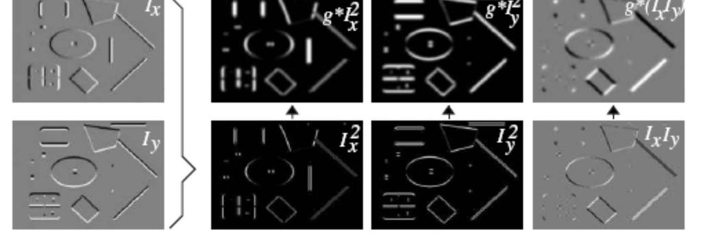
69 Harris Corner Detector - Steps 1. Compute the horizontal and vertical (Gaussian) derivatives fx Gxy (,, D)* f( xi, yi) f y Gxy (,, D)* f( xi, yi) x y σ D is called the differentiation scale 2. Compute the three images involved in A W : A W 2 fx fx f y w( x, y) 2 x W, y W fx fy fy

70 Harris Detector - Steps 3. Convolve each of the three images with a larger Gaussian w(x,y) : 4. Determine cornerness: Gaussian σ I is called the integration scale R(A W ) = det(a W ) α trace 2 (A W ) 5. Find local maxima

71 Harris Detector - Example

72 Harris Detector - Example

73 Harris Detector - Example Compute corner response R

74 Harris Detector - Example Find points with large corner response: R>threshold

75 Harris Detector - Example Take only the points of local maxima of R

76 Harris Detector - Example Map corners on the original image

77 Harris Detector Scale Parameters The Harris detector requires two scale parameters: (i) a differentiation scale σ D for smoothing prior to the computation of image derivatives, & (ii) an integration scale σ I for defining the size of the Gaussian window (i.e., integrating derivative responses). A W (x,y) A W (x,y,σ I,σ D ) Typically, σ I =γσ D

78 Invariance to Geometric/Photometric Changes Is the Harris detector invariant to geometric and photometric changes? Geometric Rotation Scale Affine Photometric Affine intensity change: I(x,y) a I(x,y) + b

79 Harris Detector: Rotation Invariance Rotation Ellipse rotates but its shape (i.e. eigenvalues) remains the same Corner response R is invariant to image rotation

80 Harris Detector: Rotation Invariance (cont d)

81 Harris Detector: Photometric Changes Affine intensity change Only derivatives are used => invariance to intensity shift I(x,y) I (x,y) + b Intensity scale: I(x,y) a I(x,y) R R threshold x (image coordinate) x (image coordinate) Partially invariant to affine intensity change

82 Harris Detector: Scale Invariance Scaling Corner All points will be classified as edges Not invariant to scaling (and affine transforms)

83 Harris Detector: Repeatability In a comparative study of different interest point detectors, Harris was shown to be the most repeatable and most informative. Repeatability = # correspondences min( m, m ) 1 2 best results: σ I =1, σ D =2 C. Schmid, R. Mohr, and C. Bauckhage, "Evaluation of Interest Point Detectors", International Journal of Computer Vision 37(2), , 2000.

84 Harris Detector: Disadvantages Sensitive to: Scale change Significant viewpoint change Significant contrast change

85 How to handle scale changes? A W must be adapted to scale changes. If the scale change is known, we can adapt the Harris detector to the scale change (i.e., set properly σ I, σ D ). What if the scale change is unknown?

86 Multi-scale Harris Detector Detects interest points at varying scales. R(A W ) = det(a W (x,y,σ I,σ D )) α trace 2 (A W (x,y,σ I,σ D )) scale σ n =k n σ σ D = σ n σ I =γσ D σ n y Harris x

87 How to cope with transformations? Exhaustive search Invariance Robustness

88 Multi-scale approach Exhaustive search Slide from T. Tuytelaars ECCV 2006 tutorial

89 Multi-scale approach Exhaustive search

90 Multi-scale approach Exhaustive search

91 Multi-scale approach Exhaustive search

92 How to handle scale changes? Not a good idea! There will be many points representing the same structure, complicating matching! Note that point locations shift as scale increases. The size of the circle corresponds to the scale at which the point was detected

93 How to handle scale changes? (cont d) How do we choose corresponding circles independently in each image?

94 How to handle scale changes? (cont d) Alternatively, use scale selection to find the characteristic scale of each feature. Characteristic scale depends on the feature s spatial extent (i.e., local neighborhood of pixels). scale selection scale selection

95 How to handle scale changes? Only a subset of the points computed in scale space are selected! The size of the circles corresponds to the scale at which the point was selected.

96 Automatic Scale Selection Design a function F(x,σ n ) which provides some local measure. Select points at which F(x,σ n ) is maximal over σ n. F(x,σ n ) max of F(x,σ n ) corresponds to characteristic scale! σ n T. Lindeberg, "Feature detection with automatic scale selection" International Journal of Computer Vision, vol. 30, no. 2, pp , 1998.

97 Invariance Extract patch from each image individually

98 Automatic scale selection Solution: Design a function on the region, which is scale invariant (the same for corresponding regions, even if they are at different scales) Example: average intensity. For corresponding regions (even of different sizes) it will be the same. For a point in one image, we can consider it as a function of region size (patch width) f Image 1 f Image 2 scale = 1/2 region size region size

99 Automatic scale selection Common approach: Take a local maximum of this function Observation: region size, for which the maximum is achieved, should be invariant to image scale. Important: this scale invariant region size is found in each image independently! f Image 1 f Image 2 scale = 1/2 s 1 region size s 2 region size

100 Automatic Scale Selection f I (, )) ( (, i x f I x )) 1 im i im ( 1 Same operator responses if the patch contains the same image up to scale factor. 100

101 Automatic Scale Selection Function responses for increasing scale (scale signature) f ( I (, )) i i 1 x i i m f ( I 1 ( x, )) m 101

102 Automatic Scale Selection Function responses for increasing scale (scale signature) f ( I (, )) i i 1 x i i m f ( I 1 ( x, )) m 102

103 Automatic Scale Selection Function responses for increasing scale (scale signature) f ( I (, )) i i 1 x i i m f ( I 1 ( x, )) m 103

104 Automatic Scale Selection Function responses for increasing scale (scale signature) f ( I (, )) i i 1 x i i m f ( I 1 ( x, )) m 104

105 Automatic Scale Selection Function responses for increasing scale (scale signature) f ( I (, )) i i 1 x i i m f ( I 1 ( x, )) m 105

106 Automatic Scale Selection Function responses for increasing scale (scale signature) f I (, )) i i i i m f ( I 1 ( x, )) m ( 1 x 106

107 Scale selection Use the scale determined by detector to compute descriptor in a normalized frame

108 Automatic Scale Selection (cont d) Characteristic scale is relatively independent of the image scale. Scale factor: 2.5 The ratio of the scale values corresponding to the max values, is equal to the scale factor between the images. Scale selection allows for finding spatial extend that is covariant with the image transformation.

109 Automatic Scale Selection What local measures should we use? Should be rotation invariant Should have one stable sharp peak

110 How should we choose F(x,σ n )? Typically, F(x,σ n ) is defined using derivatives, e.g.: Square gradient L x L x LoG L x L x : ( x(, ) y(, )) 2 : ( xx (, ) yy (, )) DoG : I( x)* G( ) I( x)* G( ) n 1 n :det( 2 W) ( W) Harris function A trace A C. Schmid, R. Mohr, and C. Bauckhage, "Evaluation of Interest Point Detectors", International Journal of Computer Vision, 37(2), pp , 2000.

111 Review Patch/Template Matching #111 Interest Points Corner Detection: Harris Detector Properties of Harris Detector Scaling approach