Motion Estimation (I) Ce Liu Microsoft Research New England

Transcription

1 Motion Estimation (I) Ce Liu Microsoft Research New England

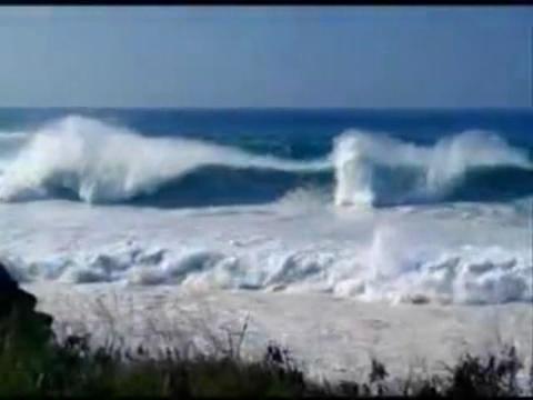
2 We live in a moving world Perceiving, understanding and predicting motion is an important part of our daily lives

3 Motion estimation: a core problem of Related topics: computer vision Image correspondence, image registration, image matching, image alignment, Applications Video enhancement: stabilization, denoising, super resolution 3D reconstruction: structure from motion (SFM) Video segmentation Tracking/recognition Advanced video editing (label propagation)

4 Contents (today) Motion perception Motion representation Parametric motion: Lucas-Kanade Dense optical flow: Horn-Schunck Robust estimation Applications (1)

5 Contents (next time) Discrete optical flow Layer motion analysis Contour motion analysis Obtaining motion ground truth SIFT flow: generalized optical flow Applications (2)

6 Readings Rick s book: Chapter 8 Ce Liu s PhD thesis (appendix A & B) S. Baker and I. Matthews. Lucas-Kanade 20 years on: a unifying framework. IJCV 2004 Horn-Schunck (wikipedia) A. Bruhn, J. Weickert, C. Schnorr. Lucas/Kanade meets Horn/Schunk: combining local and global optical flow methods. IJCV 2005

7 Contents Motion perception Motion representation Parametric motion: Lucas-Kanade Dense optical flow: Horn-Schunck Robust estimation Applications (1)

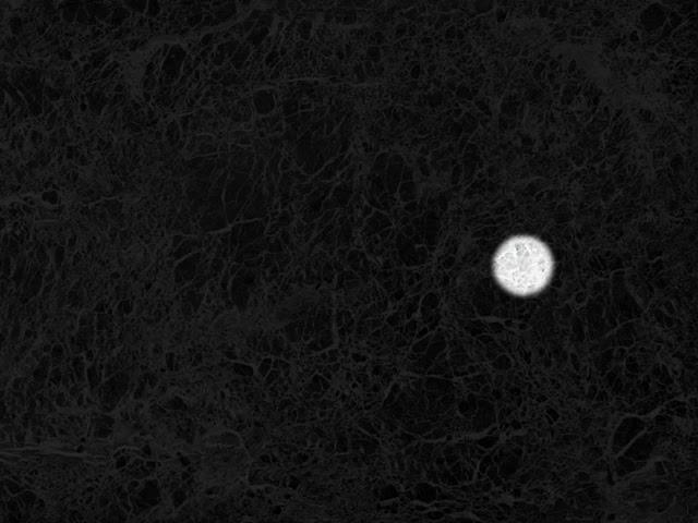
8 Seeing motion from a static picture?

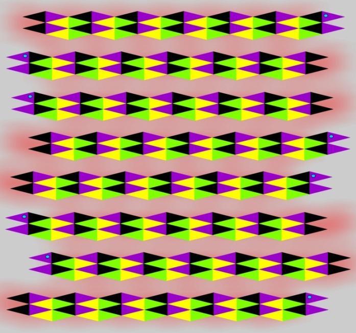
9 More examples

10 How is this possible? The true mechanism is to be revealed FMRI data suggest that illusion is related to some component of eye movements We don t expect computer vision to see motion from these stimuli, yet

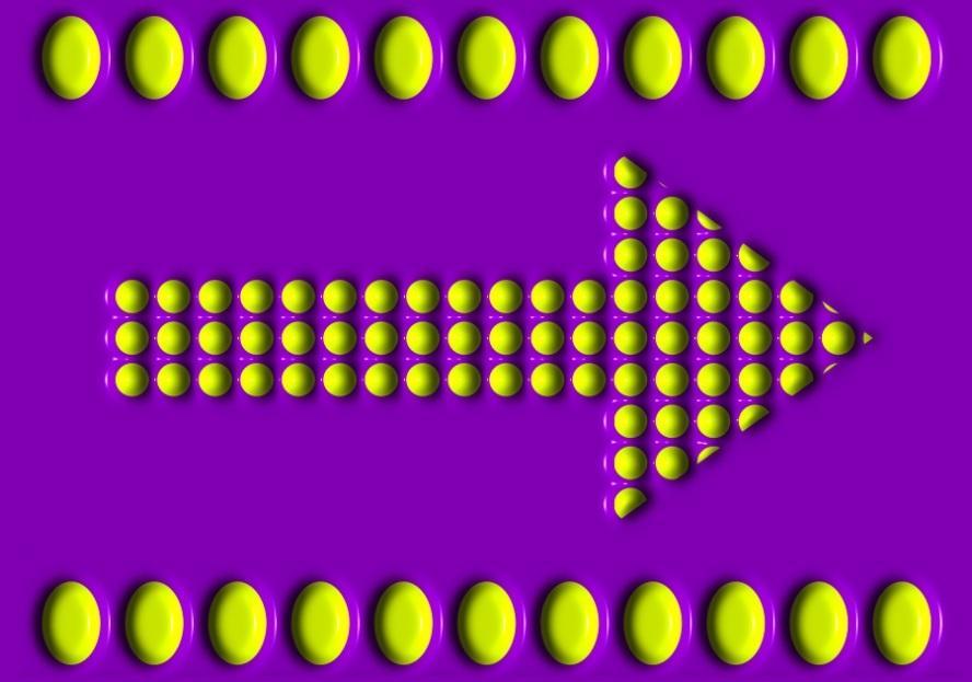
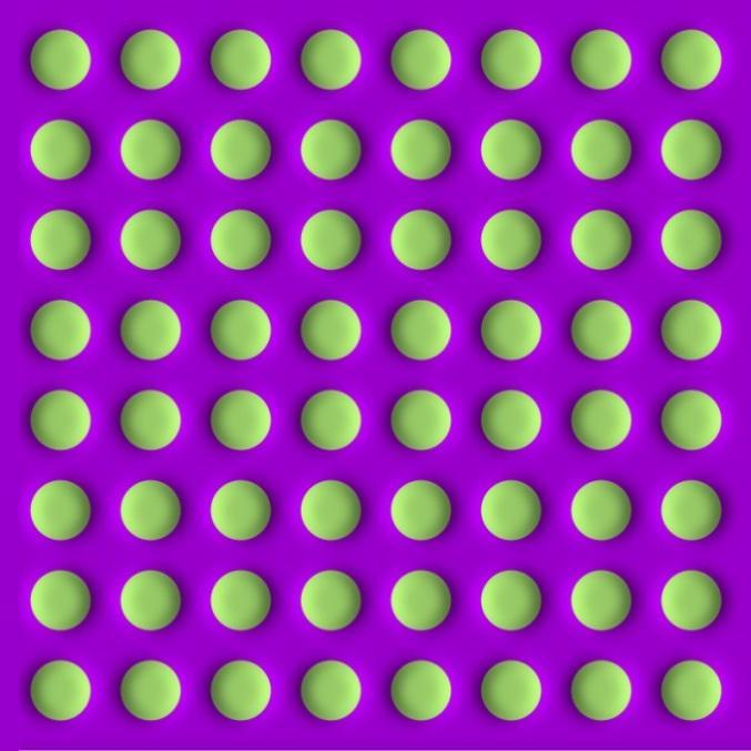
11 What do you see?

12 In fact,

13 We still don t touch these areas

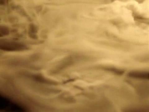
14 Motion analysis: human vs. computer Computers can only analyze motion for opaque and solid objects Challenges: Shapeless or transparent scenes Key: motion representation

15 Contents Motion perception Motion representation Parametric motion: Lucas-Kanade Dense optical flow: Horn-Schunck Robust estimation Applications (1)

16 Motion forms Mapping: x 1, y 1 (x 2, y 2 ) Global parametric motion: x 2, y 2 Motion types Translation: x 2 y 2 Similarity: x 2 y 2 Affine: x 2 y 2 = x 1 + a y 1 + b = s Homography: x 2 y 2 cos α sin α = ax 1 + by 1 + c dx 1 + ey 1 + f = 1 z sin α cos α = f(x 1, y 1 ; θ) x 1 + a y 1 + b ax 1 + by 1 + c dx 1 + ey 1 + f, z = gx 1 + y 1 + i

17 Illustration of motion types Translation

18 Optical flow field Parametric motion is limited and cannot describe the motion of arbitrary videos Optical flow field: assign a flow vector u x, y, v x, y to each pixel (x, y) Projection from 3D world to 2D

19 Optical flow field visualization Too messy to plot flow vector for every pixel Map flow vector to color Magnitude: saturation Orientation: hue Input Ground-truth flow field Visualization code [Baker et al. 2007]

20 Matching criterion Brightness constancy assumption I 1 x, y = I 2 x + u, y + v + r + g r N 0, σ 2, g U 1,1 Noise r, outlier g (occlusion, lighting change) Matching criteria What s invariant between two images? Brightness, gradients, phase, other features Distance metric (L2, L1, truncated L1, Lorentzian) E u, v = x,y ρ I 1 x, y I 2 x + u, y + v Correlation, normalized cross correlation (NCC)

21 Error functions L2 norm ρ z = z L1 norm ρ z = z Truncated L1 norm ρ z = min ( z, η) Lorentzian ρ z = log (1 + γz 2 )

22 Robust statistics Traditional L2 norm: only noise, no outlier Example: estimate the average of 0.95, 1.04, 0.91, 1.02, 1.10, Estimate with minimum error z = arg min z L2 norm: z = L1 norm: z = i ρ z z i Truncated L1: z = Lorentzian: z = L2 norm ρ z = z Truncated L1 norm ρ z = min ( z, η) L1 norm ρ z = z Lorentzian ρ z = log (1 + γz 2 )

23 Contents Motion perception Motion representation Parametric motion: Lucas-Kanade Dense optical flow: Horn-Schunck Robust estimation Applications (1)

24 Lucas-Kanade: problem setup Given two images I 1 (x, y) and I 2 (x, y), estimate a parametric motion that transforms I 1 to I 2 Let x = x, y T be a column vector indexing pixel coordinate Two typical transforms Translation: W x; p = x + p 1 y + p 2 Affine: W x; p = p 1x + p 2 y + p 3 p 4 x + p 5 y + p = p 1 p 2 p x 3 6 p 4 p 5 p y 6 1 Goal of the Lucas-Kanade algorithm p = arg min p I 2 W x; p I 1 x 2 x

25 An incremental algorithm Difficult to directly optimize the objective function p = arg min p I 2 W x; p I 1 x 2 x Instead, we try to optimize each step Δp = arg min Δp The transform parameter is updated: x I 2 W x; p + Δp I 1 x 2 p p + Δp

26 Taylor expansion The term I 2 W x; p + Δp is highly nonlinear Taylor expansion: I 2 W x; p + Δp I 2 W x; p + I 2 W p Δp W : Jacobian of the warp p If W x; p = W x x; p, W y x; p T, then W p = W x W x p 1 p n W y W y p 1 p n

27 Jacobian matrix For affine transform: W x; p = p 1 p 2 p x 3 p 4 p 5 p y 6 1 The Jacobian is W = x y p x 0 0 y 1 For translation : W x; p = x + p 1 y + p 2 The Jacobian is W p =

28 Taylor expansion I 2 = I x I y is the gradient of image I 2 evaluated at W(x; p): compute the gradients in the coordinate of I 2 and warp back to the coordinate of I 1 For affine transform W = x y p x 0 0 y 1 W I 2 p = I x x I x y I x I y x I y y I y Let matrix B = [I x X I x Y I x I y X I y Y I y ] R n 6, I x and X are both column vectors. I x X is element-wise vector multiplication.

29 Gauss-Newton With Taylor expansion, the objective function becomes Δp = arg min Δp x Or in a vector form: I 2 W x; p + I 2 W p Δp I 1 x 2 Δp = arg min Δp I t + BΔp T (I t + BΔp) Where B = [I x X I x Y I x I y X I y Y I y ] R n 6 I t = I 2 W p I 1 Solution: Δp = B T B 1 B T I t

30 Jacobian: W p = I 2 W p = I x I y B = [I x I y ] R n 2 Solution: Translation Δp = B T B 1 B T I t = I x T I x I T x I y I T x I y I T y I y 1 Ix T I t I y T I t

31 How it works

32 Coarse-to-fine refinement Lucas-Kanade is a greedy algorithm that converges to local minimum Initialization is crucial: if initialized with zero, then the underlying motion must be small If underlying transform is significant, then coarse-to-fine is a must (u 2, v 2 ) 2 Smooth & downsampling (u 1, v 1 ) 2 (u, v)

33 Variations Variations of Lucas Kanade: Additive algorithm [Lucas-Kanade, 81] Compositional algorithm [Shum & Szeliski, 98] Inverse compositional algorithm [Baker & Matthews, 01] Inverse additive algorithm [Hager & Belhumeur, 98] Although inverse algorithms run faster (avoiding recomputing Hessian), they have the same complexity for robust error functions!

34 From parametric motion to flow field Incremental flow update (du, dv) for pixel x, y I 2 x + u + du, y + v + dv I 1 x, y = I 2 x + u, y + v + I x x + u, y + v du + I y x + u, y + v dv I 1 x, y I x du + I y dv + I t = 0 We obtain the following function within a patch T I x du dv = I x I T x I y I x T I y I y T I y 1 Ix T I t I y T I t The flow vector of each pixel is updated independently Median filtering can be applied for spatial smoothness

35 Example Input two frames Coarse-to-fine LK Flow visualization Coarse-to-fine LK with median filtering

36 Contents Motion perception Motion representation Parametric motion: Lucas-Kanade Dense optical flow: Horn-Schunck Robust estimation Applications (1)

37 Motion ambiguities When will the Lucas-Kanade algorithm fail? T I x du dv = I x I T x I y I x T I y I y T I y 1 Ix T I t I y T I t The inverse may not exist!!! How? All the derivatives are zero: flat regions X- and y- derivatives are linearly correlated: lines

38 The aperture problem Corners Lines Flat regions

39 Dense optical flow with spatial regularity Local motion is inherently ambiguous Corners: definite, no ambiguity Lines: definite along the normal, ambiguous along the tangent Flat regions: totally ambiguous Solution: imposing spatial smoothness to the flow field Adjacent pixels should move together as much as possible Horn & Schunck equation u, v = arg min I x u + I y v + I t 2 + α u 2 + v 2 dxdy u 2 = u 2 u 2 + = ux 2 + u2 x y y α: smoothness coefficient Data term Smoothness term

40 2D Euler Lagrange 2D Euler Lagrange: the functional S = L x, y, f, f x, f y dxdy Ω is minimized only if f satisfies the partial differential equation (PDE) In Horn-Schunck L f x L f x y L f y = 0 L u, v, u x, u y, v x, v y = I x u + I y v + I t 2 + α ux 2 + u y 2 + v x 2 + v y 2 L u = 2 I xu + I y v + I t I x L u x = 2αu x, x L = 2αu u xx, L = 2αu x u y, y y L u y = 2αu yy

41 Linear PDE The Euler-Lagrange PDE for Horn-Schunck is I x u + I y v + I t I x α u xx + u yy = 0 I x u + I y v + I t I y α v xx + v yy = 0 u xx + u yy can be obtained by a Laplacian operator: In the end, we solve a large linear system I x 2 + αl I x I y I x I y I 2 y + αl U V = I xi t I y I t

42 How to solve a large linear system? I x 2 + αl I x I y I x I y I 2 y + αl U V = I xi t I y I t With α > 0, this system is positive definite! You can use your favorite solver Gauss-Seidel, successive over-relaxation (SOR) (Pre-conditioned) conjugate gradient No need to wait for the solver to converge completely

43 Condition for convergence In the objective function u, v = arg min I x u + I y v + I t 2 + α u 2 + v 2 dxdy The displacement (u, v) has to be small for the Taylor expansion to be valid. More practically, we can estimate the optimal incremental change I x du + I y dv + I t 2 + α u + du 2 + v + dv 2 dxdy The solution becomes I x 2 + αl I x I y I x I y I 2 y + αl du dv = I xi t + αlu I y I t + αlv

44 Examples Horn-Schunck Input two frames Coarse-to-fine LK Flow visualization Coarse-to-fine LK with median filtering

45 The source of over-smoothness Horn-Schunck is a Gaussian Markov random field (GMRF) I x u + I y v + I t 2 + α u 2 + v 2 dxdy Spatial over-smoothness is caused by quadratic smoothness term Nevertheless, optical flow fields are sparse! Horn-Schunck u u x u y v v x v y Ground truth

46 Continuous Markov Random Fields Horn-Schunck started 30 years of research on continuous Markov random fields Optical flow estimation Image reconstruction, e.g. denoising, super resolution Shape from shading, inverse rendering problems Natural image priors Why continuous? Many signals are differentiable More complicated spatial relationships Fast solvers Multi-grid Preconditioned conjugate gradient FFT + annealing

47 Contents Motion perception Motion representation Parametric motion: Lucas-Kanade Dense optical flow: Horn-Schunck Robust estimation Applications (1)

48 Modification to Horn-Schunck Let x = (x, y, t), and w x = (u x, v x, 1) be the flow vector Horn-Schunck (recall) I x u + I y v + I t 2 + α u 2 + v 2 dxdy Robust estimation ψ I x + w I x 2 + αφ u 2 + v 2 dxdy Robust estimation with Lucas-Kanade g ψ I x + w I x 2 + αφ u 2 + v 2 dxdy

49 Robust functions Various forms of robust functions L1 norm: ψ z 2 = z 2 + ε 2, φ z 2 = z 2 + ε 2 Sub L1: ψ z 2 ; η = z 2 + ε 2 η, η < 0.5 Lorentzian: ψ z 2 = log(1 + z 2 ) z z 2 + ε =0.5 =0.4 =0.3 =

50 Special cases The robust objective function g ψ I x + w I x 2 + αφ u 2 + v 2 dxdy Lucas-Kanade: α = 0, ψ z 2 = z 2 Robust Lucas-Kanade: α = 0, ψ z 2 = z 2 + ε 2 Horn-Schunck: g = 1, ψ z 2 = z 2, φ z 2 = z 2 One can also learn the filters (other than gradients), and robust function ψ, φ [Roth & Black 2005]

51 Derivation strategies Euler-Lagrange Derive in continuous domain, discretize in the end Nonlinear PDE s Outer and inner fixed point iterations Cannot generalize to general filters Variational optimization Iterative reweighted least square (IRLS) Discretize first and derive in matrix form Easy to understand and derive These three approaches are equivalent!

52 Iterative reweighted least square (IRLS) Let φ z = z 2 + ε 2 η be a robust function We want to minimize the objective function n Φ Ax + b = φ a i T x + b i 2 i=1 where x R d, A = a 1 a 2 a n T R n d, b R n By setting Φ x = 0, we can derive Φ n x = φ a T 2 i x + b i = i=1 n i=1 n w ii a i T xa i + w ii b i a i = i=1 = A T WAx + A T Wb a i T w ii xa i + b i w ii a i a i T x + b i a i w ii = φ a i T x + b i 2 W = diag Φ Ax + b

53 Iterative reweighted least square (IRLS) Derivative: Φ x = AT WAx + A T Wb Iterate between reweighting and least square 1. Initialize x = x 0 2. Compute weight matrix W = diag Φ Ax + b 3. Solve the linear system A T WAx = A T Wb 4. If x converges, return; otherwise, go to 2 Convergence is guaranteed (local minima)

54 Objective function IRLS for robust optical flow g ψ I x + w I x 2 + αφ u 2 + v 2 dxdy Discretize, linearize and increment x,y g ψ( I t + I x du + I Y dv 2 ) + αφ( u + du 2 + v + dv 2 ) IRLS (initialize du = dv = 0) Weight: Least square: Ψ xx = diag g ψ I x I x, Ψ xy = diag g ψ I x I y, Ψ yy = diag g ψ I y I y, Ψ xt = diag(g ψ I x I t ), = diag(g ψ I y I t ), L = D T x Φ D x + D T y Φ D y Ψ yt Ψ xx + αl Ψ xy + αl Ψ xy Ψ yy du dv = Ψ xt + αlu I y I t + αlv

55 Examples Robust optical flow Input two frames Horn-Schunck Flow visualization Coarse-to-fine LK with median filtering

56 Contents Motion perception Motion representation Parametric motion: Lucas-Kanade Dense optical flow: Horn-Schunck Robust estimation Applications (1)

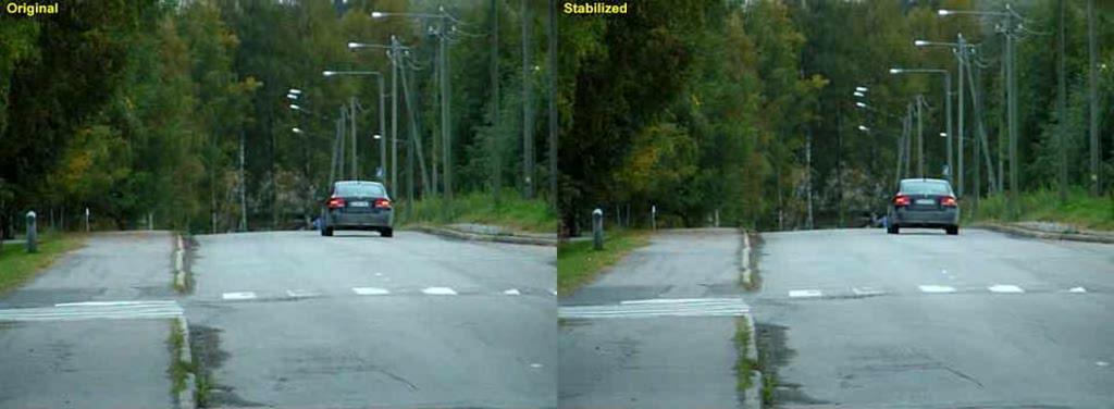
57 Video stabilization

58 Video denoising Use multiple frames for temporal coherence Non-local mean

59 Video denoising

60 Video super resolution Merge information from adjacent frames Reconstruction depends on flow accuracy

61 Summary Lucas-Kanade Parametric motion Dense flow field (with median filtering) Horn-Schunck Gaussian Markov random field Euler-Lagrange Robust flow estimation Robust function Account for outliers in data term Encourage piecewise smoothness IRLS (= nonlinear PDE = variational optimization)

62 Next time Discrete optical flow Layer motion analysis Contour motion analysis Obtaining motion ground truth SIFT flow: generalized optical flow Applications (2)