Image Analysis. Feature extraction: corners and blobs

Transcription

1 Image Analysis Feature extraction: corners and blobs Christophoros Nikou Images taken from: Computer Vision course by Svetlana Lazebnik, University of North Carolina at Chapel Hill ( D. Forsyth and J. Ponce. Computer Vision: A Modern Approach, Prentice Hall, 003. M. Nixon and A. Aguado. Feature Extraction and Image Processing. Academic Press 010. University of Ioannina - Department of Computer Science Corners and Blobs 1

2 3 Motivation: Panorama Stitching 4 Motivation: Panorama Stitching (cont.) Step 1: feature extraction Step : feature matching

3 5 Motivation: Panorama Stitching (cont.) Step 1: feature extraction Step : feature matching Step 3: image alignment 6 Characteristics of good features Repeatability The same feature can be found in several images despite geometric and photometric transformations. Saliency Each feature has a distinctive description. Compactness and efficiency Many fewer features than image pixels. Locality A feature occupies a relatively small area of the image; robust to clutter and occlusion. 3

4 7 Applications Feature points are used for: Motion tracking. Image alignment. 3D reconstruction. Object recognition. Image indexing and retrieval. Robot navigation. 8 Image Curvature Extends the notion of edges. Rate of change in edge direction. Points where the edge direction changes rapidly are characterized as corners. We need some elements from differential geometry. Parametric form of a planar curve: Ct () = [ xt (), y ()] t Describes the points in a continuous curve as the endpoints of a position vector. 4

5 9 Image Curvature (cont.) The tangent vector describes changes in the position vector: dx dy Tt () = Ct () = [ xt (), yt ()] =, dt dt Intuitive meaning think of the trace of the curve as the motion of a point at time t. The tangent vector describes the instantaneous motion. 10 Image Curvature (cont.) At any time moment, the point moves with velocity magnitude: Ct x t y t () = () + () in the direction: 1 yt () ϕ() t = tan x () t 5

6 11 Image Curvature (cont.) The curvature at a point C(t) describes the changes in the direction of the tangent with respect to changes in arc length (constant displacements along the curve): κ () t = dϕ() t ds The curvature is given with respect to the arc length because a curve parameterized by the arc length maintains a constant velocity. 1 Image Curvature (cont.) Gradient direction N(t) φ(t) Edge curve C(t) ( ) Tangent T(t) dϕ() t κ () t = ds 6

7 13 Image Curvature (cont.) Parameterization of a planar curve by the arc length is the length of the curve from 0 to t: t dc() t s() t = dt 0 dt This implies: ds() t d dc() t dc() t t = dt x t y t dt dt = = + 0 dt dt () () 14 Image Curvature (cont.) Parameterization by the arc length is not unique but it has the property: dc() t dc() t dc() t dc() t dc() t dt dt dt = = dt = = = 1 ds dt ds ds ds dc() t dt dt dt 7

8 15 Image Curvature (cont.) Back to the definition of curvature: dϕ() t dϕ() t dt κ () t = = ds dt ds d 1 y 1 = tan dt x x () t + y () t x () t y() t y () t x() t κ() t = 3/ x () t + y () t 16 Image Curvature (cont.) Some useful relations from differential geometry of planar curves (easily deduced) are: dc() t ds = Tt () dc () t ds = κ () tnt () The curvature is the magnitude of the second derivative of the curve with respect to the arc length: κ () t = dc () t ds 8

9 17 Image Curvature (cont.) It is also useful to express the normal vector at a point to a curve in Cartesian coordinates: yt () xt () Nt () =, Tt () = [ xt (), yt ()] x () t + y () t x () t + y () t 18 Image Curvature (cont.) There are three main approaches to compute curvature Direct computation on an edge image. Derive the measure of curvature from image intensities. Correlation. x () t y() t y () t x() t κ() t = 3/ x () t + y () t 9

10 19 Image Curvature (cont.) Direct computation from edges. Difference in edge direction. κ() t = ϕ( t+ 1) ϕ( t 1) with 1 yt ( + 1) yt ( 1) ϕ() t = tan xt ( + 1) xt ( 1) Connected edges are needed (hysteresis). 0 Image Curvature (cont.) Direct computation from edges. Smoothing is generally required by considering more than two pixels: n 1 κ() t = ϕ( t+ 1 + i) ϕ( t+ i 1) n i= 1 Not very reliable results. Reformulation of a first order edge detection scheme. Quantization errors in angle measurement. Threshold to detect corners. 10

11 1 Image Curvature (cont.) Direct computation from edges. Object silhouette Thresholded curvature The result depends strongly on the threshold. Image Curvature (cont.) Computation from image intensity. It should be computed along the curve (normal to the image gradient) for each pixel. Cartesian coordinates for the angle of the tangent φ(x,y). Measure of angular changes in the image with respect to location. The curve at an image point may be approximated by: ( ϕ ) ( ϕ ) x() t = x( t 1) + tcos ( x, y) yt () = yt ( 1) + tsin ( xy, ) 11

12 3 Image Curvature (cont.) Computation from image intensity. with The curvature is given by: ϕ( x, y) ϕ( x, y) x( t) ϕ( x, y) y( t) κϕ ( xy, ) = = + t x t y t xt () yt () = cos ( ϕ( x, y) ), = sin ( ϕ( x, y) ), t t 1 M x ϕ( xy, ) = tan Normal to the curve. Recall M y that this is associated with the C ss (t). 4 Image Curvature (cont.) Computation from image intensity. κ ϕ Substituting the all the terms: 1 M M y M x y M x ( xy, ) = M 3/ y MM x y + Mx MM x y x x y y ( Mx + M y) Alternatively, by differentiating backwards: 1 M M y M x y M x κ ϕ ( xy, ) = M 3/ y MM x y Mx + MM x y x x y y ( Mx + M y) 1

13 5 Image Curvature (cont.) Computation from image intensity. Other measures differentiate along the normal to the curve. The idea is that curves may be thicker than one pixel wide. Differentiating along the normal measures the difference between internal and external gradient angles. Theoretically, these are equal. However, in practice they differ due to image discretization. The more the edge is bent, the larger the difference (Kass et al. IJCV 1988). 6 Image Curvature (cont.) Computation from image intensity. The measures are: 1 M y M y M y M x κ ϕ ( xy, ) = M 3/ x MM x y MM x y + MM x y x x y y ( Mx + M y) 1 M y M M x y M x κ ϕ ( xy, ) = M 3/ x + MM x y MM x y + M y x x y y ( Mx + M y) 13

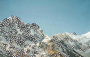
14 7 Image Curvature (cont.) Computation from image intensity. κϕ κ ϕ κ ϕ κ ϕ Better than direct computation but the results are not consistent. 8 Finding Corners Image Curvature by Correlation Key property: in the region around a corner, image gradient has two or more dominant directions. Corners are repeatable and distinctive. C.Harris and M.Stephens. "A Combined Corner and Edge Detector. Proceedings of the 4th Alvey Vision Conference: pages

15 9 The Basic Idea We should easily recognize the point by looking through a small window. Shifting a window in any direction should give a large change in intensity. flat region: no change in all directions edge : no change along the edge direction corner : significant change in all directions Source: A. Efros 30 Harris Corner Detector Change in appearance for the shift [u,v]: [ + + ] E ( uv, ) = wxy (, ) I ( x+ u, y+ v ) I ( xy, ) xy, Window function Shifted intensity Intensity Window function w(x,y) or 1 in window, 0 outside Gaussian Source: R. Szeliski 15

16 31 Harris Detector (cont.) Change in appearance for the displacement [u,v]: xy, [ ] E( uv, ) = wxy (, ) I( x+ u, y + v) I( x, y) Second-order Taylor expansion of E(u,v) around (0,0): E( u, v) E(0,0) + [ u Eu (0,0) 0) 0) Euu (0,0) Euv(0,0) u v] [ u v] Ev (0,0) Euv(0,0) Evv(0,0) v 3 Harris Detector (cont.) [ ] E( uv, ) = wxy (, ) I( x+ u, y + v) I( x, y) xy, As E(0,0)= 0, the higher order terms yield: E I( x+ u, y+ v) Eu = = wxy (, )[ Ix ( + uy, + v) Ixy (, )] u xy, u I( x+ u, y+ v) ( x+ u) = wxy (, )[ I( x+ uy, + v) I( xy, )] = ( x + u ) u x, y xy, [ ] = wxy (, ) I( x+ uy, + v) I( xy, ) I( x+ uy, + v) At the origin: E u (0,0) = 0 x 16

17 33 Harris Detector (cont.) E Eu = = wxy (, )[ Ix ( + uy, + v) Ixy (, )] Ix( x+ uy, + v) u xy, y The second order term is: E E Euu = = u u u = wxyi (, ) ( x+ uy, + vi ) ( x+ uy, + v) x xy, x [ ] + I ( x+ u, y+ v) w( x, y) I( x+ u, y+ v) I( x, y) xx At the origin: E w x y I x y uu (0,0) = (, ) x (, ) 34 Harris Detector (cont.) By the same reasoning we obtain the rest of the derivatives: E = w x y I x y uu (0,0) 0) (, ) x (, ) E w x y I x y vv (0,0) = (, ) y (, ) E (0,0) = E (0,0) = w( x, y) I ( x, y) I ( x, y) uv vu x y And the final expression becomes: 1 Euu (0,0) 0) Euv (0,0) 0) u Euv (, ) [ u v] Euv (0,0) Evv (0,0) v Ix IxI y u Euv (, ) [ u v] wxy (, ) xy, II x y I y v 17

18 35 Harris Detector (cont.) The bilinear approximation simplifies to u u E ( u, v) [ u v] M v where M is a matrix computed from image derivatives: M I x II x y = w( x, y) xy, II x y Iy M 36 Harris Detector (cont.) The surface E(u,v) is locally approximated by a quadratic form. Let s try to understand its shape. E ( u, v) [ u v] M u v M I x I x I = I xi y I y y 18

19 37 Harris Detector (cont.) First, consider the axis-aligned case where gradients are either horizontal or vertical. M = I x I xi y I I x y I y = λ1 0 0 λ If either λ is close to 0, then this is not a corner, so look for locations where both are large. 38 Harris Detector (cont.) Since M is symmetric, it can be written as: λ M = R R 0 λ We can visualize M as an ellipse with axes lengths determined by the eigenvalues and orientation determined by the rotation matrix R. Ellipse equation: u [ u v] M = const v direction of the fastest change (λ max ) -1/ (λ min ) -1/ direction of the slowest change 19

20 39 Visualization of second moment matrices 40 Visualization of second moment matrices (cont.) 0

21 41 Window size matters! 4 Interpreting the eigenvalues Classification of image points using eigenvalues of M : λ Edge λ >> λ 1 Corner λ 1 and λ are large, λ 1 ~ λ ; E increases in all directions λ 1 and λ are small; E is almost constant in all directions Flat region Edge λ 1 >> λ λ 1 1

22 43 Corner response function R = det( M ) M α trace( ) = λ1λ α( λ1 + λ ) α: constant (0.04 to 0.06) Edge R < 0 Corner R > 0 Flat region R small Edge R < 0 44 Harris detector: Steps 1. Compute Gaussian derivatives at each pixel.. Compute second moment matrix M in a Gaussian window around each pixel. 3. Compute corner response function R. 4. Threshold R. 5. Find local maxima of response function (nonmaximum suppression).

23 45 Harris Detector: Steps (cont.) 46 Harris Detector: Steps (cont.) Compute corner response R 3

24 47 Harris Detector: Steps (cont.) Find points with large corner response: R>threshold 48 Harris Detector: Steps (cont.) Take only the points of local maxima of R 4

25 49 Harris Detector: Steps (cont.) 50 Invariance Features should be detected despite geometric or photometric changes in the image: if we have two transformed versions of the same image, features should be detected in corresponding locations. 5

26 51 Models of Image Transformation Geometric Rotation Scale Affine valid for: orthographic hi camera, locally ll planar object Photometric Affine intensity change (I a I + b) 5 Rotation Harris Detector: Invariance Properties The ellipse rotates but its shape (i.e. eigenvalues) remains the same. Corner response R is invariant to image rotation 6

27 53 Harris Detector: Invariance Properties (cont.) Affine intensity change Only derivatives are used => invariance to intensity shift I I + b Intensity scale: I a I R threshold R x (image coordinate) x (image coordinate) Partially invariant to affine intensity change 54 Harris Detector: Invariance Properties (cont.) Scaling Corner All points will be classified as edges Not invariant to scaling 7

28 55 Harris Detector: Invariance Properties (cont.) Harris corners are not invariant to scaling. This is due to the Gaussian derivatives computed at a specific scale. If the image differs in scale the corners will be different. For scale invariance, it is necessary to detect features that can be reliably extracted under scale changes. 56 Scale-invariant feature detection Goal: independently detect corresponding regions in scaled versions of the same image. Need scale selection mechanism for finding characteristic region size that is covariant with the image transformation. Idea: Given a key point in two images determine if the surrounding neighborhoods contain the same structure up to scale. We could do this by sampling each image at a range of scales and perform comparisons at each pixel to find a match but it is impractical. 8

29 57 Scale-invariant feature detection (cont.) Evaluate a signature function and plot the result as a function of the scale. The shape should be similar in different scales. 58 Scale-invariant feature detection (cont.) The only operator fulfilling these requirements is a scale-normalized Gaussian. T. Lindeberg. Scale space theory: a basic tool for analyzing structures at different scales. Journal of Applied Statistics, 1(), pp. 4 70,

30 59 Scale-invariant feature detection (cont.) Based on the above idea, Lindeberg (1998) proposed a detector for blob-like features that searches for scale space extrema of a scalenormalized LoG. T. Lindeberg. Feature detection with automatic scale selection. International Journal of Computer Vision, 1(), pp. 4 70, Scale-invariant feature detection (cont.) 30

31 61 Recall: Edge Detection f Edge d dx g Derivative of Gaussian f d dx g Edge = maximum of derivative Source: S. Seitz 6 Recall: Edge Detection (cont.) f Edge d dx g Second derivative of Gaussian (Laplacian) d dx f g Edge = zero crossing of second derivative Source: S. Seitz 31

32 63 From edges to blobs Edge = ripple. Blob = superposition of two edges (two ripples). Spatial selection: the magnitude of the Laplacian response will achieve a maximum at the center of the blob, provided the scale of the Laplacian is matched to the scale of the blob. maximum 64 Scale selection We want to find the characteristic scale of the blob by convolving it with Laplacians at several scales and looking for the maximum response. However, Laplacian response decays as scale increases: original signal (radius=8) increasing σ Why does this happen? 3

33 65 Scale normalization The response of a derivative of Gaussian filter to a perfect step edge decreases as σ increases. 1 σ π 66 Scale normalization (cont.) The response of a derivative of Gaussian filter to a perfect step edge decreases as σ increases. To keep the response the same (scaleinvariant), we must multiply the Gaussian derivative by σ. The Laplacian is the second derivative of the Gaussian, so it must be multiplied by σ. 33

34 67 Effect of scale normalization Original signal Unnormalized Laplacian response Scale-normalized Laplacian response maximum 68 Blob detection in D Laplacian: Circularly symmetric operator for blob detection in D. g = g x + g y 34

35 69 Blob detection in D (cont.) Laplacian: Circularly symmetric operator for blob detection in D. Scale-normalized: g g = σ x g + y norm 70 Scale selection At what scale does the Laplacian achieve a maximum response for a binary circle of radius r? r image Laplacian 35

36 71 Scale selection (cont.) The D LoG is given (up to scale) by ( x + y σ ) e ( x + y )/ σ For a binary circle of radius r, the LoG achieves a maximum at σ = r / onse r Laplacian resp image r / scale (σ) 7 Characteristic scale We define the characteristic scale as the scale that produces a peak of the LoG response. characteristic scale T. Lindeberg (1998). "Feature detection with automatic scale selection." International Journal of Computer Vision, 30 (): pp

37 73 Scale-space blob detector 1. Convolve the image with scalenormalized LoG at several scales.. Find the maxima of squared LoG response in scale-space. 74 Scale-space blob detector: Example 37

38 75 Scale-space blob detector: Example 76 Scale-space blob detector: Example 38

39 77 Efficient implementation Approximating the LoG with a difference of Gaussians: ( xx(,, ) yy (,, )) L= G x y + G x y σ σ σ (Laplacian) DoG= Gxyk (,, σ ) Gxy (,, σ ) (Difference of Gaussians) We have studied this topic in edge detection. 78 Efficient implementation Divide each octave into an equal number K of intervals such that: 1/ K n k =, σ n = k σ 0 n= 1,..., K. Implementation by a Gaussian pyramid. D. G. Lowe. "Distinctive image features from scale-invariant keypoints. International Journal of Computer Vision 60 (), pp ,

40 79 The Harris-Laplace detector It combines the Harris operator for corner-like structures with the scale space selection mechanism of DoG. Two scale spaces are built: one for the Harris corners and one for the blob detector (DoG). A key point is a Harris corner with a simultaneously maximun DoG at the same scale. It provides fewer key points with respect to DoG due to the constraint. K. Mikolajczyk and C. Schmid, Scale and Affine invariant interest point detectors, International Journal of Computer Vision, 60(1):63-86, From scale invariance to affine invariance For many problems, it is important to find features that are invariant under large viewpoint changes. The projective distortion may not be corrected locally due to the small number of pixels. A local affine approximation is usually sufficient. 40

41 81 From scale invariance to affine invariance (cont.) Affine adaptation of scale invariant detectors. Find local regions where an ellipse can be reliably and repeatedly extracted purely from local image properties. 8 Affine Adaptation Recall: M = I I I x x y λ w( x, y) = R R, y I xi y I y 0 λ x We can visualize M as an ellipse with axis lengths determined by the eigenvalues and orientation determined by R. Ellipse equation: [ ] u u v M = const v direction of the fastest change (λ max ) -1/ (λ min ) -1/ direction of the slowest change 41

42 83 Affine adaptation example Scale-invariant regions (blobs) 84 Affine adaptation example Affine-adapted blobs 4

43 85 Affine adaptation The covarying of Harris corner detector ellipse may be viewed as the characteristic shape of a region. We can normalize the region by transforming the ellipse into a unit circle. The normalized regions may be detected under any affine transformation. 86 Affine adaptation (cont.) Problem: the second moment window determined by weights w(x,y) must match the characteristic shape of the region. Solution: iterative approach Use a circular window to compute the second moment matrix. Based on the eigenvalues, perform affine adaptation to find an ellipse-shaped window. Recompute second moment matrix in the ellipse and iterate. 43

44 87 Iterative affine adaptation K. Mikolajczyk and C. Schmid, Scale and Affine invariant interest point detectors, International Journal of Computer Vision, 60(1):63-86, Orientation ambiguity There is no unique transformation from an ellipse to a unit circle We can rotate or flip a unit circle, and it still stays a unit circle. 44

45 89 Orientation ambiguity (cont.) We have to assign a unique orientation to the keypoints in the circle: Create the histogram of local gradient directions in the patch. Assign tho the patch the orientation of the peak of the smoothed histogram. 0 π 90 Summary: Feature extraction Extract affine regions Normalize regions Eliminate rotational ambiguity Compute appearance descriptors SIFT (Lowe 04) 45

46 91 Invariance vs. covariance Invariance: features(transform(image)) = features(image) Covariance: features(transform(image)) = transform(features(image)) Covariant detection => invariant description 46