Advanced Features. Advanced Features: Topics. Jana Kosecka. Slides from: S. Thurn, D. Lowe, Forsyth and Ponce. Advanced features and feature matching

Transcription

1 Advanced Features Jana Kosecka Slides from: S. Thurn, D. Lowe, Forsyth and Ponce Advanced Features: Topics Advanced features and feature matching Template matching SIFT features Haar features 2 1

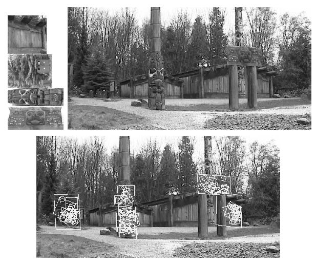
2 Features for Object Detection/Recognition Want to find in here 3 Template Convolution Pick a template - rectangular/square region of an image Goal - find it in the same image/images of the same scene from Different viewpoint 4 2

3 Convolution with Templates % read image im = imread('bridge.jpg'); bw = double(im(:,:,1))./ 255; imshow(bw) % apply FFT FFTim = fft2(bw); bw2 = real(ifft2(fftim)); imshow(bw2) % select an image patch patch = bw(221:240,351:370); imshow(patch) patch = patch - (sum(sum(patch)) / size(patch,1) / size(patch, 2)); kernel=zeros(size(bw)); kernel(1:size(patch,1),1:size(patch,2)) = patch; FFTkernel = fft2(kernel); % define a kernel kernel=zeros(size(bw)); kernel(1, 1) = 1; kernel(1, 2) = -1; FFTkernel = fft2(kernel); % apply the kernel and check out the result FFTresult = FFTim.* FFTkernel; result = real(ifft2(fftresult)); imshow(result) % apply the kernel and check out the result FFTresult = FFTim.* FFTkernel; result = max(0, real(ifft2(fftresult))); result = result./ max(max(result)); result = (result.^ 1 > 0.5); imshow(result) % alternative convolution imshow(conv2(bw, patch, 'same')) 5 Template Convolution 6 3

4 Feature Matching with templates Given a template - find the region in the image with the highest matching score Matching score - result of convolution is maximal (or use SSD, SAD, NSS similarity measures) Given rotated, scaled, perspectively distorted version of the image Can we find the same patch (we want invariance!) Scaling - NO Rotation - NO Illumination - depends Perspective Projection - NO CS223b 7 Efficient Template matching Convolution theorem: F( I g) = F( I) F( g) Fourier Transform of g: F( g( x, y))( u, v) = g( x, y) exp{ i2π ( ux + vy)} dx dy R 2 F is invertible Convolution is a spatial domain is a multiplication in frequency domain - often more efficient when fast FFT available 8 4

5 Convolution with Templates % read image im = imread('bridge.jpg'); bw = double(im(:,:,1))./ 256;; imshow(bw) % apply FFT FFTim = fft2(bw); bw2 = real(ifft2(fftim)); imshow(bw2) % define a kernel kernel=zeros(size(bw)); kernel(1, 1) = 1; kernel(1, 2) = -1; FFTkernel = fft2(kernel); % apply the kernel and check out the result FFTresult = FFTim.* FFTkernel; result = real(ifft2(fftresult)); imshow(result) % select an image patch patch = bw(221:240,351:370); imshow(patch) patch = patch - (sum(sum(patch)) / size(patch,1) / size(patch, 2)); kernel=zeros(size(bw)); kernel(1:size(patch,1),1:size(patch,2)) = patch; FFTkernel = fft2(kernel); % apply the kernel and check out the result FFTresult = FFTim.* FFTkernel; result = max(0, real(ifft2(fftresult))); result = result./ max(max(result)); result = (result.^ 1 > 0.5); imshow(result) % alternative convolution imshow(conv2(bw, patch, 'same')) 9 Feature Matching with templates Given a template - find the region in the image with the highest matching score Matching score - result of convolution is maximal (or use SSD, SAD, NSS similarity measures) Given rotated, scaled, perspectively distorted version of the image Can we find the same patch (we want invariance!) Scaling Rotation Illumination Perspective Projection 10 5

6 Improved Invariance Handling Want to find in here 11 SIFT Features Invariances: Scaling Rotation Illumination Deformation Provides Good localization Yes Yes Yes Not really Yes 12 6

7 SIFT Reference Distinctive image features from scale-invariant keypoints. David G. Lowe, International Journal of Computer Vision, 60, 2 (2004), pp SIFT = Scale Invariant Feature Transform 13 Invariant Local Features Image content is transformed into local feature coordinates that are invariant to translation, rotation, scale, and other imaging parameters SIFT Features 14 7

8 Advantages of invariant local features Locality: features are local, so robust to occlusion and clutter (no prior segmentation) Distinctiveness: individual features can be matched to a large database of objects Quantity: many features can be generated for even small objects Efficiency: close to real-time performance Extensibility: can easily be extended to wide range of differing feature types, with each adding robustness 15 SIFT On-A-Slide 1. Enforce invariance to scale: Compute Gaussian difference max, for many different scales; non-maximum suppression, find local maxima: keypoint candidates 2. Localizable corner: For each maximum fit quadratic function. Compute center with sub-pixel accuracy by setting first derivative to zero. 3. Eliminate edges: Compute ratio of eigenvalues, drop keypoints for which this ratio is larger than a threshold. 4. Enforce invariance to orientation: Compute orientation, to achieve rotation invariance, by finding the strongest second derivative direction in the smoothed image (possibly multiple orientations). Rotate patch so that orientation points up. 5. Compute feature signature: Compute a "gradient histogram" of the local image region in a 4x4 pixel region. Do this for 4x4 regions of that size. Orient so that largest gradient points up (possibly multiple solutions). Result: feature vector with 128 values (15 fields, 8 gradients). 6. Enforce invariance to illumination change and camera saturation: Normalize to unit length to increase invariance to illumination. Then threshold all gradients, to become invariant to camera saturation. 16 8

9 Finding Keypoints (Corners) Idea: Find Corners, but scale invariance Approach: Run linear filter (difference of Gaussians) Do this at different resolutions of image pyramid 17 Difference of Gaussians Minus Equals Approximates Laplacian (see filtering lecture) 18 9

10 Difference of Gaussians surf(fspecial('gaussian',40,4)) surf(fspecial('gaussian',40,8)) surf(fspecial('gaussian',40,8) - fspecial('gaussian',40,4)) im =imread('bridge.jpg'); bw = double(im(:,:,1)) / 256; for i = 1 : 10 gaussd = fspecial('gaussian',40,2*i) - fspecial('gaussian',40,i); res = abs(conv2(bw, gaussd, 'same')); res = res / max(max(res)); imshow(res) ; title(['\bf i = ' num2str(i)]); drawnow end 19 Gaussian Kernel Size i=

11 Gaussian Kernel Size i=2 21 Gaussian Kernel Size i=

12 Gaussian Kernel Size i=4 23 Gaussian Kernel Size i=

13 Gaussian Kernel Size i=6 25 Gaussian Kernel Size i=

14 Gaussian Kernel Size i=8 27 Gaussian Kernel Size i=

15 Resample Blur Subtract Gaussian Kernel Size i=10 29 Key point localization In D. Lowe s paper image is decomposed to octaves (consecutively sub-sampled versions of the same image) Instead of convolving with large kernels within an octave kernels are kept the same Detect maxima and minima of differenceof-gaussian in scale space Look for 3x3 neighbourhood in scale and space 30 15

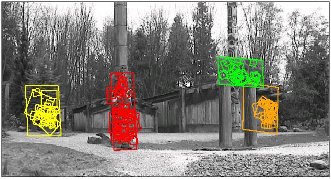
16 Example of keypoint detection (a) 233x189 image (b) 832 DOG extrema (c) 729 above threshold 31 SIFT On-A-Slide 1. Enforce invariance to scale: Compute Gaussian difference max, for may different scales; non-maximum suppression, find local maxima: keypoint candidates 2. Localizable corner: For each maximum fit quadratic function. Compute center with sub-pixel accuracy by setting first derivative to zero. 3. Eliminate edges: Compute ratio of eigenvalues, drop keypoints for which this ratio is larger than a threshold. 4. Enforce invariance to orientation: Compute orientation, to achieve rotation invariance, by finding the strongest second derivative direction in the smoothed image (possibly multiple orientations). Rotate patch so that orientation points up. 5. Compute feature signature: Compute a "gradient histogram" of the local image region in a 4x4 pixel region. Do this for 4x4 regions of that size. Orient so that largest gradient points up (possibly multiple solutions). Result: feature vector with 128 values (15 fields, 8 gradients). 6. Enforce invariance to illumination change and camera saturation: Normalize to unit length to increase invariance to illumination. Then threshold all gradients, to become invariant to camera saturation

17 Example of keypoint detection Threshold on value at DOG peak and on ratio of principle curvatures (Harris approach) (c) 729 left after peak value threshold (from 832) (d) 536 left after testing ratio of principle curvatures 33 SIFT On-A-Slide 1. Enforce invariance to scale: Compute Gaussian difference max, for may different scales; non-maximum suppression, find local maxima: keypoint candidates 2. Localizable corner: For each maximum fit quadratic function. Compute center with sub-pixel accuracy by setting first derivative to zero. 3. Eliminate edges: Compute ratio of eigenvalues, drop keypoints for which this ratio is larger than a threshold. 4. Enforce invariance to orientation: Compute orientation, to achieve rotation invariance, by finding the strongest second derivative direction in the smoothed image (possibly multiple orientations). Rotate patch so that orientation points up. 5. Compute feature signature: Compute a "gradient histogram" of the local image region in a 4x4 pixel region. Do this for 4x4 regions of that size. Orient so that largest gradient points up (possibly multiple solutions). Result: feature vector with 128 values (15 fields, 8 gradients). 6. Enforce invariance to illumination change and camera saturation: Normalize to unit length to increase invariance to illumination. Then threshold all gradients, to become invariant to camera saturation

18 Select canonical orientation Create histogram of local gradient directions computed at selected scale Assign canonical orientation at peak of smoothed histogram Each key specifies stable 2D coordinates (x, y, scale, orientation) 0 2π 35 SIFT On-A-Slide 1. Enforce invariance to scale: Compute Gaussian difference max, for may different scales; non-maximum suppression, find local maxima: keypoint candidates 2. Localizable corner: For each maximum fit quadratic function. Compute center with sub-pixel accuracy by setting first derivative to zero. 3. Eliminate edges: Compute ratio of eigenvalues, drop keypoints for which this ratio is larger than a threshold. 4. Enforce invariance to orientation: Compute orientation, to achieve rotation invariance, by finding the strongest second derivative direction in the smoothed image (possibly multiple orientations). Rotate patch so that orientation points up. 5. Compute feature signature: Compute a "gradient histogram" of the local image region in a 4x4 pixel region. Do this for 4x4 regions of that size. Orient so that largest gradient points up (possibly multiple solutions). Result: feature vector with 128 values (15 fields, 8 gradients). 6. Enforce invariance to illumination change and camera saturation: Normalize to unit length to increase invariance to illumination. Then threshold all gradients, to become invariant to camera saturation

19 SIFT vector formation Thresholded image gradients are sampled over 16x16 array of locations in scale space Create array of orientation histograms 8 orientations x 4x4 histogram array = 128 dimensions CS223b 37 Nearest-neighbor matching to feature database Hypotheses are generated by approximate nearest neighbor matching of each feature to vectors in the database SIFT use best-bin-first (Beis & Lowe, 97) modification to k-d tree algorithm Use heap data structure to identify bins in order by their distance from query point Result: Can give speedup by factor of 1000 while finding nearest neighbor (of interest) 95% of the time 38 19

20 3D Object Recognition Extract outlines with background subtraction 39 3D Object Recognition Only 3 keys are needed for recognition, so extra keys provide robustness Affine model is no longer as accurate 40 20

21 Recognition under occlusion 41 Test of illumination invariance Same image under differing illumination 273 keys verified in final match 42 21

22 Examples of view interpolation 43 Location recognition 44 22

23 SIFT Invariances: Scaling Yes Rotation Yes Illumination Yes Perspective Projection Maybe Provides Good localization Yes 45 SOFTWARE for Matlab (at UCLA, Oxford)

24 SIFT demos Run sift_compile sift_demo