Visual Object Recognition

Transcription

1 Visual Object Recognition Lecture 2: Image Formation Per-Erik Forssén, docent Computer Vision Laboratory Department of Electrical Engineering Linköping University

2 Lecture 2: Image Formation Pin-hole, and thin lens cameras Projective geometry, lens distortion, vignetting, intensity, colour Geometric and Photometric Invariance Colour constancy, colour spaces, affine illumination model, homographies, epipolar geometry, canonical frames

3 The Pin-Hole Camera A brightly illuminated scene will be projected onto a wall opposite of the pin-hole. The image is rotated 180º.

4 The Pin-Hole Camera Optical Centre ( ) X= X Y Y Z y x f x y z Z X From similar triangles we get: x = f X Z y = f Y Z 2 3 x 4y5 = 1 2 f f X 4Y 5 Z

5 The Pin-Hole Camera 2 3 x 4y5 = 1 2 f f X 4Y 5 Z More generally, we write: 2 3 x 4y5 = f s c x X 40 fa c 5 4 y Y Z f-focal length, s-skew, a-aspect ratio, c-projection of optical centre

6 The Pin-Hole Camera 2 3 x 4y5 = f s c x X 40 fa c 5 4 y Y Z Motivation: Optical Centre z Image Plane f-focal length, s-skew, a-aspect ratio, c-projection of optical centre y f O FOV o FOV x Image Grid w c ( x c y ) h

7 The Pin-Hole Camera 2 3 x 4y5 1 {z} x = f s c x X 40 fa c 5 4 y Y {z 1 Z } {z } K X, x K X Motivation: Optical Centre z Image Plane f-focal length, s-skew, a-aspect ratio, c-projection of optical centre y f O FOV o FOV x Image Grid w c ( x c y ) h

8 The Pin-Hole Camera x 4y 5 1 {z} x = f s c x 40 fa c y Also normalized image coordinates: u = 5 {z } K 2 3 X/Z 4Y/Z5 1 X 4Y 5 Z {z } X, x K X x = Ku K X u = K 1 x

9 The Pin-Hole Camera For a general position of the world coordinate system (WCS) we have: u r 11 r 12 r 13 t 1 4r 21 r 22 r 23 t 5 2 r 31 r 32 r 33 {z t 3 } [R t] X 6Y 4Z {z } X

10 The Pin-Hole Camera For a general position of the world coordinate system (WCS) we have: u r 11 r 12 r 13 t 1 4r 21 r 22 r 23 t 5 2 r 31 r 32 r 33 {z t 3 } [R t] X 6Y 4Z {z } X, u [R t]x

11 The Pin-Hole Camera For a general position of the world coordinate system (WCS) we have: u and thus r 11 r 12 r 13 t 1 4r 21 r 22 r 23 t 5 2 r 31 r 32 r 33 {z t 3 } [R t] x K[R t]x X 6Y 4Z {z } X, u [R t]x

12 Epipolar geometry The epipolar geometry of two cameras: epipolar plane ( X= X ) Y Z o 1 o 2 e e 2 baseline 1 camera 1 camera 2 x 1 epipolar lines x 2 e 1, e 2 are called epipoles. o 1,o 2 are the optical centres.

13 Homographies For a planar object, we can imagine a world coordinate system fixed to the object y x f Optical Centre x y z Z X Y ( X= X ) Y x 4y5 = K r 11 r 12 r 13 t 1 4r 21 r 22 r 23 t 5 2 r 31 r 32 r 33 t 3 2 X 6Y 4Z

14 Homographies For a planar object, we can imagine a world coordinate system fixed to the object y x f Optical Centre x y z Z X Y ( X= X ) Y x 4y5 = K r 11 r 12 t 1 4r 21 r 22 t 5 2 r 31 r 32 t 3 X 4Y = 2 3 h 11 h 12 h 13 4h 21 h 22 h 5 23 h 31 h 32 h 33 {z } H 2 3 X 4Y 5 1

15 Homographies Projections into two cameras: As the homography is invertible, we can now map from camera 2 to the object and on to camera 1:

16 Epipolar Geometry So in general, two view geometry only tells us that a corresponding point lies somewhere along a line. In practice, we often know more, as objects often have planar, or near planar surfaces. i.e., we are close to the homography case. Also: If the views have a short relative baseline, we can use even more simple models.

17 Thin Lens Camera An actual pinhole lets in too little light, and a bigger hole blurs the picture. Real cameras instead use lenses to obtain a sharp image using more light.

18 Thin Lens Camera A thin lens is a (positive) lens with Focal point f Optical Centre d << f Parallel rays converge at the focal points d Rays through the optical centre are not refracted

19 Thin Lens Camera Image plane Focal point Optical Centre Focal point f d Z l Thin lens relation (from similar triangles): 1 f = 1 Z + 1 l

20 Thin Lens Camera Image plane Focal point Optical Centre Focal point l f d Z Focus at one depth only. Objects at other depths are blurred.

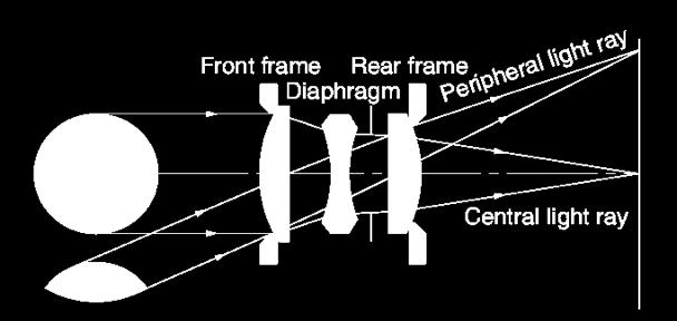
21 Thin Lens Camera Image plane Aperture Focal point Optical Centre Focal point l f Adding an aperture increases the depth-of-field, the range which is sharp in the image. A compromise between pinhole and thin lens. d Z

22 Lens distortion Correct Barrel distortion Pin-cushion distortion For zoom lenses: - Barrel at wide FoV - pin-cushion at narrow FoV

23 Lens distortion ) Correct image Distorted Modelling x Kf(u, 0 ) Used in optimisation such as BA

24 Lens distortion ) Distorted image Correct Rectification x 0 f 1 (Ku, ) Used in dense stereo

25 Lens Effects Correct Darkened periphery Vignetting and cos 4 -law - more severe on wide angle cameras

26 Lens Effects Vignetting cos 4 -law dampening with cos 4 (w)

27 Image intensity Sensor activation is linear Z a(x) = s( )r(, x)e( )d s-sensor absorption spectrum, r-reflectance spectrum of object, e- emission spectrum of light source (attenuated by the atmosphere)

28 Image intensity Sensor activation is linear Z a(x) = s( )r(, x)e( )d s-sensor absorption spectrum, r-reflectance spectrum of object, e- emission spectrum of light source (attenuated by the atmosphere) However, most images are gamma corrected i(x) =a(x)

29 Image intensity Sensor activation is linear Z a(x) = s( )r(, x)e( )d HVS handles a dynamic range on Exposure time and aperture size also scale the activation. Unless we know all aspects of image formation, we cannot trust the absolute intensity value.

30 Colour Colour perception is done using three different activation functions

31 Colour Colour perception is done using three different activation functions Sensor activation is not colour. Colour is an object property, i.e. a representation of. In order to estimate colour, we need to somehow compensate for the illumination.

32 Invariance Transformations varying illumination Two categories of nuisance factors for recognition/matching varying camera pose

33 Invariance Transformations varying illumination varying camera pose For matching we need either to know the changes, or an invariance transformation Ideally, an invariance transformation should keep information intrinsic to the object, but remove all influence from the imaging process

34 Invariance Transformations Photometric invariance gives robustness to illumination changes Geometric invariance gives robustness to view changes varying illumination varying camera pose

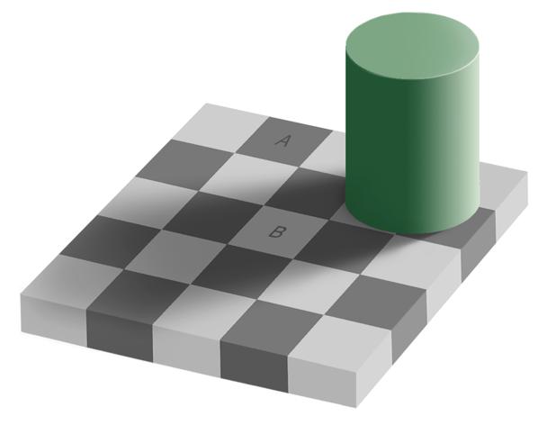
35 Colour Constancy

36 Colour Constancy

37 Colour Constancy The colours we perceive are not the activations of cones in the retina. Colour constancy is an attempt by the HVS to transform the retinal activation into a normalized (white) reference illumination. Complex process that takes place at many levels (retina, V2, ) and uses high level information (e.g. known object colour). White balancing in cameras is a low-level technical equivalent.

38 Colour Constancy Object based colour transfer If you know what you are looking at, you also know something about the illumination Forssén & Moe, View Matching with Blob Features, JIVC 09

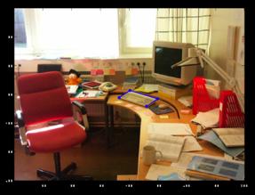
39 Photometric invariance I(x) =k 1 I 0 (x) J(x) =k 2 I 0 (x) Input If illumination changes, direct matching fails X I(x) J(x) = large x

40 Photometric invariance I(x) =k 1 I 0 (x) J(x) =k 2 I 0 (x) Input If illumination changes, direct matching fails X I(x) J(x) = large x We seek a function that is invariant to scalings X f(i(x)) f(j(x)) = small x

41 Photometric invariance For cameras with non non-linear radiometric response (and e.g. gamma correction), or if two different cameras are used we may use the affine model: I(x) =k 1 I 0 (x)+k 0 How should we choose f? we want: X x f(i(x)) f(j(x)) = small

42 Photometric invariance Mean subtraction, derivatives, and other DC free linear filters remove a constant offset in intensity Normalising a patch by e.g. the standard deviation, removes scalings of the intensity. Affine invariance by combining both: f(i(x)) = (I(x) µ I )/ I µ I = mean of patch I = std of patch

43 Photometric invariance Illustration Input Gradient Normalised gradient Normalised input I(x) J(x)

44 Other colour spaces Transform each pixel separately Move intensity change into one dimension. E.g. HSV space. In matching, V is then downweighted (or discarded)

45 Other colour spaces Other popular choices are the CIE Lab space (left) and the Yuv space. Colour space changes do not handle changes in the illumination colour.

46 Geometric invariance The geometric invariances we use make a locally planar assumption. (see also today s paper) They can thus be described using homographies.

47 Geometric invariance A homography is a transformation between points x on one plane, and points y on another y 1 y = H 4 x 1 x = h 11 h 12 h 13 4h 21 h 22 h 23 h 31 h 32 h 33 At most 8 degrees-of-freedom (dof) as H and kh,k 2 R \ 0 define the same transformation See e.g. R. Hartley and A. Zisserman, Multiple View Geometry for Computer Vision 5 3 x 1 4x 5 2 1

48 Geometric invariance A hierarchy of transformations: scale+translation (3dof) similarity (4dof) (scale+translation+rotation) affine (6dof) (similarity+skew) plane projective (8dof) (affine+forshortening) 2 3 s 0 t 1 40 s t c s t 1 s c t a 11 a 12 t 1 4a 21 a 22 t h 11 h 12 h 13 4h 21 h 22 h 23 5 h 31 h 32 h 33

49 Canonical Frames Aka. covariant frames, and invariant frames. Resample patches to canonical frame. Points from e.g. Harris detector, or DoG maxima.

50 Canonical Frames After resampling matching is much easier!

51 Canonical Frames Combinatoral issues From Harris or DoG we get images full of keypoints.

52 Canonical Frames Combinatoral issues From Harris or DoG we get images full of keypoints. Using the points, we want to generate frames in both reference and query view and match them. We don t want to miss a combination in one of the images, but we don t want to generate too many combinations either.

53 Canonical Frames Solutions: Use each point as a reference point. Restrict frame construction to k-nearest neighbours in scale space (or image plane). Remove duplicate groupings, and reflections.

54 Summary Photometric invariance is needed to handle changes in illumination. Common approaches: colour constancy, other colour spaces, and normalisation Geometric invariance handles changes in object pose A locally planar assumption is very useful for geometric invariance

55 Discussion Questions/comments on paper: M. Brown, D. Lowe, "Invariant Features from Interest Point Groups", BMVC 2002 PhD students only, round robin scheduling