Intensity Transformations and Spatial Filtering: WHICH ONE LOOKS BETTER? Intensity Transformations and Spatial Filtering: WHICH ONE LOOKS BETTER?

Transcription

1 : WHICH ONE LOOKS BETTER? 3.1 : WHICH ONE LOOKS BETTER? 3.2 1

2 Goal: Image enhancement seeks to improve the visual appearance of an image, or convert it to a form suited for analysis by a human or a machine. Image enhancement does not, however, seek to restore the image, nor increase its information contents Peculiarity: actually, there is some evidence which suggests that a distorted image can be more pleasing than a perfect image! 3.3 Information Content Suppose a source, e.g. an image generates a discrete set of independent messages (grey levels) r k, with probabilities p k, k=1,...,l. Then the information associated with r k is defined as I k =-log 2 p k bits Since the sum of p k s is 1 and each p k 1, I k is nonnegative. This definition also implies that the information conveyed is large when an unlikely message is generated

3 Major Problem in Image Enhancement: the lack of a general standard dof image quality makes it very difficult to evaluate the performance of different IE schemes. Thus, Image Enhancement algorithms are mostly application-dependent, subjective and often ad- hoc. Therefore, mostly subjective criteria are used in evaluating image enhancement algorithms. 3.5 Subjective Criteria Used in Image Enhancement A. Goodness scale: how good an image is B. Impairment scale: how bad the degradation is in an image Overall goodness Group goodness scale not noticeable (1) scale just noticeable (2) Excellent (5) Best (7) definitely noticeable but only slight impairment (3) impairment acceptable (4) Good (4) Well above average (6) somewhat objectionable (5) definitely objectionable (6) Fair (3) Slightly above average (5) extremely objectionable (7) Poor (2) Average (4) Unsatisfactory (1) Slightly below average (3) Well below average (2) Worst (1) the numbers in parenthesis indicate a numerical weight attached to the rating

4 Spacial Domain: g(x, = T[f(x,] f(x, is the original image, g(x, is the output image and T[.] is an operator on f defined over a neighborhood of (x,. Special case: neighborhood size is 1 pixel T[.] is called 3.7 intensity or mapping transformation function. Lack of contrast 3.8 4

5 Contrast Stretching Poor contrast is the most common defect in images and is caused by reduced d and/or nonlinear amplitude range or poor lighting conditions. A typical contrast stretching transformation is shown below (examples are given later): v v c v b γ β v a α 0 a b L u 3.9 Contrast Stretching A special case of contrast stretching is illustrated above (bi-level output) and is called thresholding

6 Basic Grey Level Transformations s = T[r] 3.11 Image Negative s = L -1 - r r is the input grey level, s is the output grey level and L-1 is the maximum value of r

7 Log Transformation s = c log(1+r) c is a constant and r 0. This transformation maps a narrow range of low gray-level input values into a wider range of output levels. USE: Expand values of dark pixels in an image while 3.13 compressing higher level values. Inverse log will do the opposite Power-Law transformations s = cr γ (c and γ are positive constants)

8 Power-law Transformation: Gamma Correction 3.15 Power-Law Transformation for MR Image Enhancement Magnetic Resonance (MR) image of a fractured human spine

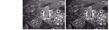
9 Power-Law Transformation for Aerial Image Original aerial image has a washed-out appearance, i.e. compression of grey levels is needed Piecewise-Linear Transformations 1. Contrast Stretching a scanning electron microscope image of pollen magnified 700 times

10 Piecewise-Linear Transformations 2. Level slicing an input image result after applying transformation in (a). Applications: enhancing features, e.g. masses of water in satellite imagery 3.19 and enhancing flaws in X-ray images. Piecewise-Linear Transformations, another example 10

11 3. Bit-plane Slicing Piecewise-Linear Transformations Bit-plane Slicing: example 1:

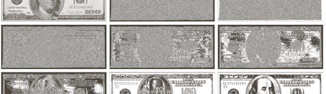
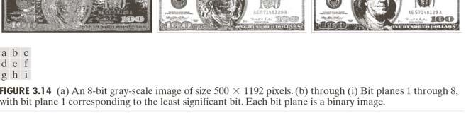
12 Bit-plane Slicing: Example 2: 12

13 Histogram Processing Basic image types: dark light low-contrast high-contrast 3.25 Histogram Processing Histogram processing re-scales an image so that the enhanced image histogram follows some desired form. The modification can take on many forms: histogram equalization, or histogram shaping e.g. exponential or hyperbolic histogram

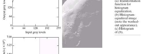
14 Histogram Equalization To transfer the gray levels so that the histogram of the resulting image is equalized to be a constant: The purpose: to equally use all available gray levels; This figure shows that for any given mapping function between the input and output images, the following holds: i.e., the number of pixels mapped from x to y is unchanged Histogram Equalization To equalize the histogram of the input image, we let p( be a constant. Assume that the gray levels are in the range of 0 and 1 (0<x<1, 0<y<1). Then we have: i.e., the mapping function for histogram equalization is: where is the cumulative probability distribution of the input image, which is monotonically non-decreasing function

15 Histogram Equalization Histogram equalization is based on the following idea: If p(x) is large, y=f(x) has a steep slope, dy will be wide, causing p( to be low; If p(x) is small, y=f(x) has a shallow slope, dy will be narrow, causing p( to be high Histogram Equalization For discrete gray levels, the gray level of the input takes one of the discrete values; and the continuous mapping function: becomes discrete: where Pi is the probability for the gray level of any given pixel to be (0<i<L):

16 Histogram Equalization The resulting function is in the range and it needs to be converted to the gray levels by one of the two following ways: where is the floor, or the integer part of a real number x, and adding 0.5 is for proper rounding. Note that while both conversions map to the highest gray level L - 1, the second conversion also maps to 0 to stretch the gray levels of the output image to occupy the entire dynamic range Histogram Equalization Example: Assume the images have pixels in 8 gray levels. The following table shows the equalization process corresponding to the two conversion methods above: 0/ / / / / / / / / / /7 5/ / / / / /7 7/7 6/ /7 7/7 7/ / / y 1 j=[y (L-1)+0.5], y 2 j=[(y -y min)/(1-y min) (L-1) +0.5],

17 Intensity Transformations and Histogram Equalization 3.33 Histogram Equalization In the following example, the histogram of a given image is equalized. Although h the resulting histogram may not look constant, but the cumulative histogram is a exact linear ramp indicating that the density histogram is indeed equalized. The density histogram is not guaranteed to be a constant because the pixels of the same gray level cannot be separated to satisfy a constant distribution

18 Histogram Equalization Programming Hints: Find histogram of given image: Build lookup table: Image Mapping: 3.35 Histogram Equalization Histogram equalization produces an output image by point re- scaling such that the histogram of the new image is uniform. Assume an image R of size M=NxN. Let # pixels with value rj H R ( j) = M where j=1,2,..., J. H R (j) is just the fractional number of pixels whose amplitude is quantized to reconstruction level r j. We want to produce an enhanced image S whose histogram (normalized) is 1 H S ( i) = i = 1,2,..., K K i.e. a histogram that is as flat as possible

19 Histogram Equalization The scaling algorithm: 1. compute the average value of the histogram. 2. starting at the lowest gray level of the original, combine pixels in the quantization bands until the sum is closest to the average. 3. Rescale all of these pixels to the first reconstruction level at the midpoint of the enhanced image first quantization band. 4. Repeat for higher gray level values Histogram Equalization Remark: 1Hi 1. Histogram equalization i works best on images with ih details hidden in dark regions. 2. Good quality originals are usually degraded when their histograms are equalized. 3. Other histogram modifications are possible, ex. a useful one is called histogram hyperbolization

20 Histogram Equalization 4. However, a normalized image histogram is just an approximation of the image probability density function! Therefore, histogram modification is nothing but modification of the underlying pdf! E.g., in histogram equalization, the enhanced image is desired to have a uniform p.d.f. That is, if p r (r) is the pdf of the original image r, then the pdf p s (s) of the enhanced image s is uniform. This is not a difficult probability problem: Consider a random variable (RV) R with pdf p R (r) and cumulative distribution function (cdf) P R (r). Find a transformation T(.) such that the new RV S=T(R) is uniform, i.e., p S (s) is a uniform density Histogram Equalization Claim: S=T(R)= P R (r) will do it. Proof: r S = PR ( r) = pr ( t) dt 0 Let's find the cdf of S (P S (s)). Stop/Resume P ( s) = Pr ob[ P ( r) s] = Pr ob[ R P S P 1 ( s) R R = 1 pr ( t) dt = PR ( PR ( s)) = s 0 for 0 s 1. 1 R ( s)]

21 Histogram Equalization In discrete case, becomes S = P R ( r) = r 0 p R ( t) dt for k=0,1,...,l-1.,, s k = T ( r ) = k k j= 0 p ( r ) = R j k j= 0 n j n (*) 3.41 Histogram Equalization any transformation such as plotted above can be used as a transformation provided that it is single valued and monotonically increasing, and it takes values in [0,1] for inputs in [0,1]

22 Histogram Equalization 3.43 Histogram Equalization s k = T ( r ) = k k j= 0 p ( r ) = R j k j= 0 n j n (*)

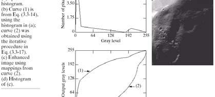
23 3.45 Histogram Equalization Photo of the Mars moon Phobos and its higtogram g

24 Histogram Equalization

25 Localized Histogram Equalization

26 3.51 m S ( x, σ S ( x, ( 1, E) E. f ( x, if ms x, < k0mg and k1σ G < σs( x, < k g( x, = f ( x, otherwise ( 2σG

27 E. f ( x, if ms x, < k0mg and k1σ G < σs( x, < k g( x, = f ( x, otherwise ( 2σG 3.53 Enhancement using logic operations AND OR

28 Enhancement using arithmetic operations 3.55 Note: Fig. 3.14(a) is the original picture in 3rd ed. 28

29 Enhancement using arithmetic operations 3.57 Enhancement using spatial averaging operations When images are displayed (or printed), they often have suffered from noise and interferences from several sources including: electrical sensor noise, photographic grain noise, and channel errors. These noise effects can usually be removed by simple ad hoc noise-cleaning techniques applied to local neighborhoods of input pixels

30 Enhancement using spacial averaging operations Consider a noisy image: g ( x, y ) = f ( x, y ) + η ( x, y ) where the second term is noise which is uncorrelated with the input and has zero mean. Then, averaging K different noisy images: K 1 g ( x, y ) = g i ( x, y ) K i = 1 produces an output image with [ g( x, ] = f ( x, and σ σ η E g = K 3.59 Enhancement using averaging operations original i noisy image, N(0,64 2 ) result of aver 8 noisy images 16 noisy images 64 noisy images 128 noisy images

31 K=8 K=16 K=64 notice how the noise variance is decreasing with increasing K. K= Each pixel u(m,n) is replaced by a weighted average of its neighbourhood pixels

32 Linear Filtering g( x, M N ( m, n ) f ( x + m, y + m = M n= = N M w n ) m= M n= N where g(x, is the output image and f(x, is the input image. In the mask above, M=N=1. N w( m, n) 3.63 Consider again a noisy image: Spacial averaging operations g ( x, y ) = f ( x, y ) +η ( x, y ) in where the second term is noise which is uncorrelated with the input and has zero mean. Let s apply a local averaging filter (all weights are equal) with size K=(2M+1)x(2N+1): 1 1 g( x, g( x, = K ( x, W K produces an output image with = ( x, W f ( x, +η out ( x, σ = 2 out in K σ Therefore, if the input is constant over W, the SNR has improved by a factor of K!!

33 3.65 original 3 x 3 mask 5 x 5 mask 9 x 9 mask 15 x 15 mask 35 x 35 mask

34 Linear Filtering Example Image from the hubble space telescope in orbit around the Earth. Here, we want to blur the image in order to see large objects Q: What happen when important details must be preserved or the noise is non-gaussian? A: may consider a number of techniques: median and order statistics filtering, sharpening spacial filters directional filtering, i unsharp masking hybrid combinations

35 Nonlinear Filtering Median or order statistics filters may perform much better in the presence of non-gaussian noise (Nonlinear Signal Processing course!) 3.69 Sharpening Spacial Filters (subtract pixels from right to left) (subtract 1st derivative again from right to left)

36 First Order Derivative Second Order Derivatives Sharpening Spacial Filters First order derivative produces thicker edges has stronger response to grey-level steps Second order derivative has a much stronger response to details produces a double response at step changes in grey level has a stronger response to a line than to a step and to a point than to a line. Conclusion Second derivative is more useful to enhance image details 3.71 Sharpening Spacial Filters: Laplacian Isotropic 2nd order derivative (Laplacian) In digital form: 2 f 2 2 x f f f = x y = f ( x + 1, + f ( x 1, 2 f ( x, in the x-direction and in the y-direction: 2 f 2 y 2-D Laplacian: 2 = f ( x, y + 1) + f ( x, y 1) 2 f ( x, 2 2 f f = 2 2 x 2 f + 2 y this can be implemented using the mask in the next slide

37 isotropic for rotations in increments of 90 * 45 negatives of the above two masks 3.73 Sharpening Spacial Filters: Laplacian Enhancement using Laplacian: 2 f ( x, g( x, = 2 f ( x, + f ( x, f ( x, if the mask center coeff is negative if the mask center coeff is positive

38 image of the north pole of the moon result of filtering with the 45 o mask Laplacian image scaled for display purpose enhanced image 3.75 The previous expression : 2 f ( x, g( x, = 2 f ( x, + Sharpening Spacial Filters: Laplacian f ( x, f ( x, if the mask center coeff is negative if the mask center coeff is positive The above two operations can be combined and thus simplified: g ( x, y ) = 5 f ( x, y ) [ f ( x + 1, y ) + f ( x 1, y ) + f ( x, y + 1) + f ( x, y 1)] This operation can be implemented using the mask in the next slide

39 90 45 SEM image results for the 90 results for the 45 Notice how much sharper it is! 3.77 Laplacian with high-boost filtering gives better results if the original image is darker than desired, see example in next slide

40 b Sharpening Spacial Filters: First Derivative, the Gradient First derivatives are implemented using the magnitude of the gradient. The gradient is given by: f Gx f = = f x G y y The magnitude of the gradient is given by: f = mag 2 1/ / 2 f f ( f ) = [ G ] x + G y = + x y note that components of the gradient are linear operators, but the magnitude is not! Also the partial derivatives are not isotropic, but the magnitude is! The magnitude can be (for implementation reasons) approximated by: f G x + G y

41 f(x, Roberts cross-gradient operator (2x2) } f z9 z5 + z8 z6 } Sobel operators (3x3) Gy Gx

42 Combining spatial enhancement methods original Laplacian of orig ginal Single technique may not produce desirable results Must thus devise a strategy for the given application at hand This application: nuclear whole body scan want to detect deseases, e.g. bone infection and tumors original+ Laplacian Strategy: Sobel of orig use Laplacian to highlight details, gradient to enhance edges, grey-level trans. to increase dynamic range 3.83 smoothed Sobel Mask obtained by: (orig + Lap) x (smoothed Sobel) orig + mask Final result power law to orig. + mask

43 Digital Image Processing, 3rd ed. Gonzalez & Woods Chapter 3 Intensity Transformations & Self-study: Section 3.8. Using Fuzzy Techniques for Intensity Transformations and R. C. Gonzalez & R. E. Woods 43