Image Segmentation: Definition Importance. Digital Image Processing, 2nd ed. Chapter 10 Image Segmentation.

Transcription

1 : Definition Importance

2 Detection of Discontinuities: 9 R = wi z i= 1 i

3 Point Detection: 1. A Mask 2. Thresholding R T

4 Line Detection: A Suitable Mask in desired direction Thresholding Line i : R R, j i j

5 Example: -45º Mask Thresholding

6 Edge Detection: Two Mathematical model

7 f x 2 f 2 x

8 Noise Problem: f f x 2 f 2 x N ( 0,0) N ( 0,0.1) N ( 0,1) N ( 0,10)

9 Gradient Operators: f Gx x f = G = f y y 2 2 f f f f f = + + x y x y α ( x y), tan G 1 y = Gx 1 2

10 Gradient Operators: Roberts Cross Gradients: x ( ) ( ) G = z z G = z z 9 5 y 8 6 ( ) ( ) 2 2 f z9 z5 + z8 z 6 f z z + z z Roberts Cross Gradient : Prewitt Operators: y ( ) ( ) ( ) ( ) 1 2 ( 2 ) ( 2 ) ( 2 ) ( 2 ) Gx = z + z + z z + z + z G = z + z + z z + z + z G = z + z + z z + z + z G = z + z + z z + z + z variation x y

11 Gradients Operators Y-Direction X-Direction

12 Diagonal Edge 45-Direction -45-Direction

13 Original G x G Gx + Gy y

14 Pre- Smoothing 5 5 Original G x G x y y G + G

15 º and -45º lines

16 Laplacian as an isotropic Detector: f x f y f = Discrete Implementation: 2 4N's: f = 4z5 ( z2 + z4 + z6 + z8 ) 2 8N's: f = 4z ( z + z + z + z + z + z + z + z )

17 Laplacian of Gaussian (LoG): 2 r h( r) = exp 2 2σ r σ r h( r) = exp 4 2 σ 2σ

18 Original Sobel GLPF Laplacian LoG LoG>T ZC Zero Crossing: Thinner Edge Easy to compute Noise Reduction capability Spaghetti Effect (isolated circles)

19 Edge Linking (Local Processing) (, ) ( 0, 0 ) (, ) α (, ) f x y f x y E α x y x y A 0 0 Input G y G x Results

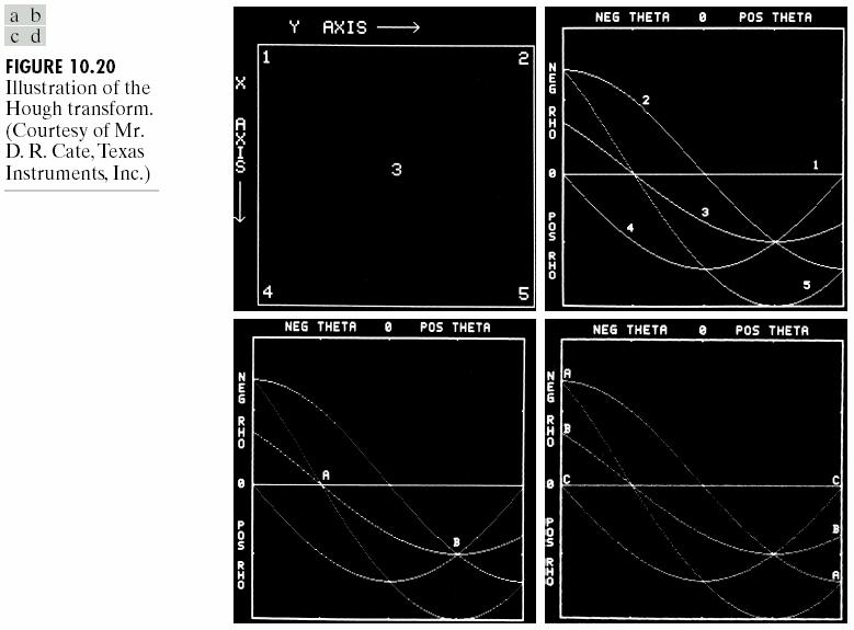
20 Global Edge Linking by the Hough Transform: ( ) x, y & y = ax + b y = ax + b i i i i b = x a + y i i ( x y ) ( ) All, 's on a line intersect each other at a,b i i

21 Hough Transform in Cartesian ( a,b ) ( x,y ) 1 1 ( x,y ) 2 2 ( x,y ) 4 4 ( x,y ) 3 3

22 Hough Transform in Polar Problem with Vertical line (a= ) ( xi, yi ) & x cos + y sin = xi cos + yi sin = ( ρi, θi ) All ( x, y )'s on a sin intersect each other at ( ρ, θ ) θ θ ρ θ θ ρ i i i i

23

24 Hough Transform

25 Hough Transform for circle: ( xi, yi ) & ( x p1 ) + ( y p2 ) = p3 ( xi p1 ) + ( yi p2 ) = p3 All ( x, y )'s on a spherical surface intersect each other at ( p, p, p ) i i Extract each circle (independent of radius): xi = p1 + r cosθ p1 = xi r cosθ p2 = p1 tanθ xi tanθ + y yi = p2 + r sinθ p2 = yi r sinθ i

26 Hough Transform for circle:

27 Hough Transform for circle:

28 Hough Transform Implementation: Discrete Accumulator Smoothing Find Local Maxima

29 Original Thr-Grad. H-T Linked

30 Thresholding: F(x,y)>T then (x,y) is belong to object, else (x,y) is belong to background. Bi-level (T) Multi-level (T 1,T 2,, T n ) Threshold image: 1 f x, y > T g ( x, y) = 0 f ( x, y) T Threshold Estimation : Histogram ( )

31 Thresholds

32 Role of illumination (, ) = (, ) (, ) f x y i x y r x y Histogram Distortion (, ) = (, ) (, ) (, ) = ln (, ) (, ) = (, ) + (, ) f x y i x y r x y z x y f x y z x y i x y r x y r ( x, y) r ( ) P r i ( x, y) Broadness Homomorphic Process i ( x, y) r ( x, y) Pf ( f )

33 Basic Global Thresholding: T = MAX + 2 min

34 How to select T: A Heuristic approach: 1. Initial guess on T 2. Segment image to G 1 (>T) and G 2 ( T) 3. Compute average value of G 1 (Ψ 1 ) and G 2 (Ψ 2 ) 4. Set T be average of Ψ 1 and Ψ 2 5. Repeat 2-4 until small changed in successive T values.

35 Convergence T0 = 0 T f = 125.4

36 Adaptive Thresholding: Local Thresholding: Subdivide the images into smaller block. Optimal Global Thresholding: Determine best value when no evidence valley.

37 Global Thr. Mosaic Local Thr.

38 Sub-image selection effect Good Subimage Bad Subimage Further block-ing

39 Optimal Global-Adaptive Thresholding: Gaussian Histogram ( ) ( z µ ) ( z µ ) σ 2 2σ 2 1 exp 2 exp P z = P + P 2 AT + BT + C = A = σ σ for σ B = 2 Pσ C = σ µ σ µ + 2σ σ ln ( µ 1σ 2 µ 2σ 1 ) P2 σ1 µ + µ σ P = = σ 2 T ln 2 µ 1 µ 2 P2

40 Optimal Global-Adaptive Thresholding: Histogram Modeling ( ) = ( ) + ( ) p z P p z P p z P + P = min T T ( ) + ( ) P p z dz P p z dz T ( ) ( ) P p T = P p T

41 Example: Preprocessing Log function( radiological absorption) Digital Subtraction (Pre and Post images) Image summation in order to reduce noise. Before After

42 Example: Optimal Thresholding: Subdivide images to 7 7 sub-block (50% overlap) Histogram Estimation Test of bimodality and Gaussian fitting and Bimodal Unimodal

43 Example: Thresholding Segmentation Boundary Detection Superimposing

44 How to improve the former methods: Consider pixels near boundary for histogram. Use of gradient/laplacian to estimate boundary: 0 f < T 2 S ( x, y) = + 1 f T and f 0 < 0: Not on Edge +1:Dark side of edge -1: Bright side of edge 2 1 f T and f 0

45 Example:

46 S(x,y) with T=midpoint Histogram of Gradient (Those with G>5)

47 Segmentation with Multiple Variables: RGB/Multi-Channel data Cluster of point in 3D Original (Color) Facial tones RED channel

48 Region Based Segmentation: n R i= 1 i R are connected regions. i R R =, i j i ( ) P R = i ( ) i Rj j TRUE P R = FALSE

49 Region Growing: Select a start (seed) point Grow the point based on a certain property Connectivity should be considered. Seed point selection: Handy Highlighted point (Due to specific property)

50 Region Growing:

51 Region Growing (Example): Determine seed points to maximum gray level. Growing criteria: Gray level value difference (with respect to S.P.) less than a threshold. Each candidate pixel should be N 8 of region.

52 Region Growing: Seed Point High Value (255) Points

53 Multimodal Histogram Threshold

54 Splitting and Merging: Define a criteria for each region to be a valid segment. Split each region which is not satisfy the criteria. Merge two neighbor region based on criteria.

55 Splitting and Merging

56 Splitting-Merging Algorithm Criteria: 80% of all pixels satisfy: z m 2σ j i i

57

58

59

60

61

62

63 The Use of Motion in Segmentation: Spatial Domain Frequency Domain Spatial Domain: Main idea: Compare pixel by pixel (difference) d ij ( x, y) ( ) ( ) Dynamic Objec 1 f x, y, ti f x, y, t j > T = 0 O.W. Static Object t

64 Accumulative Difference Image (ADI): n (,, ) f ( x, y, t1 ) { } 1 Consider f x y t i and as reference i= frame. ADI compare reference frame with incoming frame. Increment counter of each pixel when a difference detected. ADI alternative: Absolute Positive Negative

65 Accumulative Difference Image (ADI): A P k k N k ( x, y) ( x, y) ( x, y) (, ) 1 (,, ) (,, k ) ( x, y) O.W. Ak 1 x y + f x y t1 f x y t > T = Ak 1 (, ) 1 (,, ) (,, k ) ( x, y) O.W. Pk 1 x y + f x y t1 f x y t > T = Pk 1 (, ) 1 (,, ) (,, k ) ( x, y) O.W. Nk 1 x y + f x y t1 f x y t < T = Nk 1

66 ADI Example Absolute Positive Negative

67 Establishing a Reference Images: Difference will erase static object: When a dynamic object move out completely from its position, the back ground in replaced.

68 Frequency Domain Methods: A Static/black background A Dynamic single pixel x y M 1 N 1 ( ) ( ) g t a f x y t e t K j2π a1x t, =,,, = 0,1,2,, 1 1 x= 0 y= 0 N 1 M 1 ( ) ( ) g t a f x y t e t K j2π a2 y t, =,,, = 0,1, 2,, 1 2 y= 0 x= 0 K 1 1 G u a g t a e u K x ( ) ( ) j2 πu1t / K, =,, = 0,1, 2,, x 1 1 K t= 0 1 G u a g t a e u K 1 ( ) ( ) j2 πu2t / K, =,, = 0,1 y 2 1 y y 2 K t= 0 u = a v, u = a v , 2,, K 1

69 An Example:

70 Intensity Plot

71

72