THE UNIVERSITY OF OKLAHOMA GRADUATE COLLEGE THE VALUE OF REPROCESSING LEGACY DATA: A CASE STUDY OF BOIS

Transcription

1 THE UNIVERSITY OF OKLAHOMA GRADUATE COLLEGE THE VALUE OF REPROCESSING LEGACY DATA: A CASE STUDY OF BOIS D ARC, A MISSISSIPPI PLAY IN NORTHEASTERN OKLAHOMA A THESIS SUBMITTED TO THE GRADUATE FACULTY in partial fulfillment of the requirements for the Degree of MASTER OF SCIENCE By MARK AISENBERG Norman, Oklahoma 2013

2 THE VALUE OF REPROCESSING LEGACY DATA: A CASE STUDY OF BOIS D ARC, A MISSISSIPPI PLAY IN NORTHEASTERN OKLAHOMA A THESIS APPROVED FOR THE CONOCOPHILLIPS SCHOOL OF GEOLOGY AND GEOPHYSICS BY Dr. Kurt J. Marfurt, Chair Dr. Randy Keller Dr. Matthew Pranter

3 Copyright by MARK BENJAMIN AISENBERG 2013 All Rights Reserved.

4 ACKNOWLEDGEMENTS I could not have this thesis without the help of many people. First, I would like to thank the ConocoPhillips School of Geology and Geophysics at the University of Oklahoma for allowing me the chance to attain a Master s degree in Geophysics. Dr. Kurt J. Marfurt has been instrumental in my development as a student, scientist and person. Dr. Randy Keller and Dr. Matthew Pranter have both been outstanding pillars of support in my quest. In addition, Kim Guyer, Phil Hall, Isaac Hall and Andrew Peery were essential in the advice and knowledge they provided to me. Mark Falk, Michael Lovell, Jessica Griffin, Amanda Trumbo, Rika Burr, Alicia Dye, Davar Jamali, Mike Horn, Albert Babarski, Nathan Babcock, Larry Lunardi, Chris Rigsby and Tim Taylor all have given me fantastic advice in my days at Chesapeake Energy. Second, I give gratitude to Crawley Petroleum and Daniel Trumbo for providing to me the data that I used in this thesis. Data is a valuable commodity and it should not be understated. Students without data are like birds without wind. I would never have been able to take the first step without the staircase on which to climb. Without the data, I could not have executed my study and for this, you have my eternal gratitude. Many students at the university have also aided in the research and production of this manuscript. Those students include Lanre Aboaba, Alfredo Fernandez, Oswaldo Davogustto, Ben Dowdell, Shiguang Guo, Dalton Hawkins, Melia da Silva, Daniel Sigward, Daniel Trumbo, Sumit Verma and Bradley Wallet, Bo Zhang. I would also like to thank former students such as iv

5 Miguel Angelo, Rachel Barber, Toan Dao, Yoryenys Del Moro, Olubunmi Elebiju, Nabanita Gupta, Ha T. Mai, Atish Roy, Carlos Russian, Victor Pena, Roderick Perez, Xavier Refunjol, Yoscel Suarez, Aliya Urazimanova, Trey White and Kui Zhang. I have learned something from each and every one of you at some point in my career and for this I thank you. I would also like to thank Landmark for the use of ProMAX, Hampson- Russell for donating software to the University, Seis-See for the adoption of freeware to view the data as well as Schlumberger for their support of the computer room. I will always be indebted to you. Also, I would like to acknowledge the dearly departed Tim Kwiatkowski. He will always hold a special place in my memory, there was not a single person that I know who had a bigger influence on me from undergraduate to graduate student both personally and professionally. The world is a worse place without him. Finally, I want to thank my wife, Katie. She is the most special person in the world to me and made many sacrifices to allow me to perform this study. She is the world to me and without her, this degree would be meaningless. v

6 TABLE OF CONTENTS ACKNOWLEDGEMENTS...iii LIST OF TABLES...vii LIST OF FIGURES...viii ABSTRACT...xvi CHAPTER 1: INTRODUCTION...1 CHAPTER 2: GEOLOGIC BACKGROUND...6 REGIONAL...6 LOCAL GEOLOGIC SETTING...14 CHAPTER 3: 3D PRESTACK SEISMIC PROCESSING...25 DATA ACQUISTION...25 AMPLITUDE BALANCING PRESTACK TIME MIGRATION...49 CHAPTER 4 COMPARISON OF ORIGINAL PROCESSED DATA...52 CHAPTER 5: ACOUSTIC IMPEDANCE INVERSION...65 THEORY...65 PETROPHYSICAL PROPERTIES...69 ACOUSTIC IMPEDANCE INVERSION...73 CHAPTER 6: CONCLUSIONS...83 REFERENCES...85 APPENDIX A: SPECTRAL ENHANCEMENT ROUTINE...88 vi

7 LIST OF TABLES Table 1 Acquisition Parameters 27 Table 2 Analysis Windows for each well used in Multiple Attribute Regression...77 Table 3 The top 8 attributes and their error calculated during Multiple Attribute Regression analysis vii

8 LIST OF FIGURES Figure 1. Map of Oklahoma where the red outline shows Kay County and the blue inset box shows the approximate location of the survey. (Modified from the OGS, 2013)...2 Figure 2. From early Paleozoic until the Pennsylvanian uplift, Oklahoma was characterized by three major geologic provinces. The Oklahoma basin was a broad, relatively flat basin that encompassed the entire region while the Southern Oklahoma Aulacogen was enclaved by the Oklahoma basin and was the primary depocenter. The Ouachita Trough flanks both provinces in the south east and is comprised of deep marine sediments (Johnson and Cardott, 1992)...8 Figure 3. Map showing the delineation of the five major provinces of the Southern Oklahoma Aulacogen which include the Anadarko Basin, the Ardmore Basin, the Marietta Basin, the Arbuckle uplift and the Wichita Criner Uplift. (Northcutt et al., 1997) 10 Figure 4. A paleographic map showing the position of Oklahoma with respect to the North American Craton during the (a) Early Mississippian, (b) Middle-Late Mississippian and (c) the Pennsylvanian-Early Permian (modified from Blakey, 2011).16 Figure 5. Watney (2001) describes a depositional model that places Kay County on the edge of a paleo shelf margin. The Nemaha Ridge and Central Kansas Uplift delineate the edge of distinct basins with differing amounts of Atokan, Morrowan and Osagian sediments preserved today...17 viii

9 Figure 6. Column representing Oklahoma deposition stratigraphy from Precambrian to the present day (Johnson and Cardott, 1992)..18 Figure 7. Location and thickness of Misener Sandstone (Amsden, 1972).20 Figure 8. (a) A calcite rich shelf margin is deposited in shallow seas. Erosion from wave action and transport down the slope leads to a detrital mud matrix. (b) Diagenesis of the mud matrix by replacing the calcite with Silica (c) Second stage diagenesis occurs when the sub aerially exposed mud matrix is infiltrated by meteoric water, leading to a tight cherty carbonate (Modified from Rogers, 2001).22 Figure 9. (a) A calcite rich sub aerially exposed carbonate is infiltrated by meteoric rain leading to vug, karst and high porosity. (b) Transgression leads to shallow seas infiltrating the porous rock followed by diagenetic replacement of calcite with Silica (c) Second stage diagenesis occurs when the sub aerially exposed carbonate is infiltrated by meteoric water, replacing remaining calcite with silica, leading to porous tripolitic chert (Modified from Rogers, 2001) 23 Figure 10. Source and Receiver layout of the Bois d Arc merged seismic survey. Shot lines run NE-SW while receiver lines run E-W..26 Figure 11. Representative shot record sorted by channel. The signal is strong but the direct arrivals (indicated by yellow arrows) are dominant while the ground roll (indicated by green arrows) overprints traces with small source-receiver offset 29 Figure 12. FFID 8508 was one of 762 records that had been originally processed with incorrect geometry information during the original processing. The green arrow indicates the expected time of the first arrival with respect to the source-receiver offset that was in the original header. The inset picture maps the location of the live receivers ix

10 for FFID The yellow arrow indicates receivers that were properly mapped in the original processing...29 Figure 13. Surface elevation for the source and receivers of this survey. The elevation in Kay County is largely a function of the subsurface geology and as such, is something to be keenly aware of during processing. Also, elevation will play a large role in refraction statics...31 Figure 14. Map showing the maximum fold is 64, reached in the southwest corner of the survey. The nominal fold across most of the survey ranges between 30 and Figure 15. Blue arrow indicates Air blast of shot record 137 sorted by absolute offset. The air blast has a velocity of 334 m/s and is removed using ProMAX s air blast attenuation. (a)before and (b) after attenuation.33 Figure 16. Representative shot gather previously displayed in figure 15. Ground roll has a dominant velocity of 1,000 m/s in this survey and a dominant frequency of less than 20 Hz. The blue, yellow and red arrows denote the before and after removal of ground roll via a cascaded approach that included 3D FKK, Multi-window bandpass filter and mean filter spectral shaping. The orange arrow points to air blast while the green arrow points to the first break energy. (a) before cascaded noise attenuation and (b) after 33 Figure 17. Representative shot record sorted by channel before deconvolution. The raw spectrum contains signal out to ~120 Hz, the yellow arrow indicates P-wave reflection signal while the blue arrow signals low frequency head waves..35 x

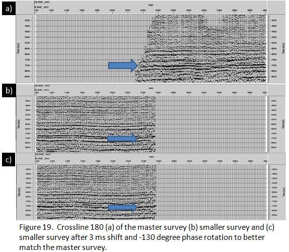
11 Figure 18. Timeslice of the two unmerged, stacked datasets using a preliminary deconvolution operator and window, a preliminary velocity, and preliminary residual statics...38 Figure 19. Crossline 180 (a) of the master survey (b) smaller survey and (c) smaller survey after 3 ms shift and -130 degree phase rotation to better match the master survey...38 Figure 20. Representative first break picks (green) 39 Figure 21. Position histograms for possible error. (a) Receiver error and (b) source error I visually inspected all shot and receiver records that were predicted by Seismic Studio to be in error by over 25 m (82.5 ft). In this manner, I was able to fine tune the geometry and find all remaining errors. The red line indicates shots and receivers showing more than 25.2 m error...41 Figure 22. Vertical slice through the velocity model. The blue arrow denotes the weathering layer while the pink arrow indicates the base of weathering. The base of weathering was held to a constant velocity of 1300 m/s while the weathering layer was variable 41 Figure 23. Stacked inline using (a) refraction statics and (b) elevation statics..42 Figure 24. Line BB after (a) refraction statics and (b) elevation statics...42 Figure 25. Refraction statics applied to (a) receivers and (b) sources 43 Figure 26. Representative shot record with the green line showing the top and bottom of the deconvolution window. The key to picking a deconvolution window is to start below the first break energy (denoted by the blue arrow), encompass as much P-wave xi

12 reflection energy as possible without making the window so long that it violates the stationary wavelet assumption.43 Figure 27. Autocorrelation corresponding to the shot gather shown in the previous figure. The blue arrow indicates a very strong correlation at time 0 while the yellow arrows indicate that the cyclical nature of the autocorrelation is virtually zero after about 140 ms, suggesting an operator length of at least 140 ms.45 Figure 28. The wavelet and spectrum corresponding to the shot record shown in the previous figure (a) before and (b) after spiking deconvolution. Note the spectrum is wider and flatter while the resultant wavelet is much better resolved with respect to time..47 Figure 29. The shot record shown previously (a) before and (b) after deconvolution. The yellow arrow indicates a zone where the signal has become much better resolved. The blue arrow indicates how the residual ground roll has been suppressed..47 Figure 30. Velocity analysis is time consuming but extremely important. I was able to pick at a density of 630 m (blue circles) which was dense enough to resolve subsample statics. A-A is a cross section of velocity analysis. Red Line indicates time of velocity time slice..48 Figure 31. Semblance velocity analysis for a 3X3 supergather containing 300 traces 50 Figure 32. The blue X s indicate receiver statics after the first iteration of residual static analysis with a standard deviation of 8 ms. Red pluses represent the second iteration of residual statics with a standard deviation of about 2 ms. Green triangles represent the xii

13 third and final pass of residual statics. The standard deviation is reduced to less than 1 ms...51 Figure 33. Line CC through the original post stack migration from The red horizon indicates the Mississippi reflector. This version adequately delineates large faults, structural highs and potential hydrocarbon traps. However, many of the subtle features are lost during this original processing flow..53 Figure 34. Post stack migration processing using the geometry QC, velocity, statics and deconvolution described in the previous Figures. The red horizon indicates the Mississippi reflection, which is now more readily visible..54 Figure 35. The prestack time migration significantly improves vertical resolution. The faults and folds are laterally confined while very steeply dipping reflectors are readily recognized. The red horizon indicates the Mississippi...55 Figure 36. Time slices at t=0.650s near the Checkerboard horizon through the (a) originally (b) reprocessed poststack time migrated and (c) reprocessed prestack time migrated and spectrally enhanced data volumes.58 Figure 37. k x -k y plot of (a) the originally processed data (b) the poststack migration with spectral enhancement and (c) the prestack time migration. The footprint in the original processing is very strong; it is partially mitigated in the poststack migration with spectral enhancement but is virtually gone in the prestack time migration 59 Figure 38. Horizon slices along the Mississippi Lime through similarity volumes computed from (a) the original 1998 stack (b) poststack time migrated and (c) the prestack time migrated volumes. The blue arrow denotes the large fault in the western part of the survey.61 xiii

14 Figure 39. Horizon slices along the top of the Mississippi Lime through volumetric dip magnitude computed from (a) original 1998 stack (b) poststack time migrated and (c) prestack time migrated volumes..62 Figure 40. Horizon slices along the top of the Mississippi through long wavelength most positive principal curvature volumes computed from (a) original 1998 (b) poststack time migrated and (c) prestack time migrated volumes..63 Figure 41. Blind well correlation with the poststack acoustic impedance inversion of the (a) originally processed data and (b) blind well correlation with the prestack acoustic impedance inversion.64 Figure 42. Synthetic log correlation for well A showing correlation of for the original processing (b) for the new spectrally enhanced poststack migration and (c) for the new prestack time migration 64 Figure 43. Demonstration of the non-uniqueness of seismic inversion. (a) An 80 foot shale between two sandstone layers, (b) a sandstone on top of a faster sandstone layers but with a 90 degree wavelet, (c) a faster shale and sandstone than in (a) but the ratio between the two is the same, demonstrating the low frequency problem (see text). (d) Tuning thickness can also cause amplitude anomalies (modified from Hampson, 1991) 66 Figure 44. Horizon slice of the four horizons used in the inversion. All 4 horizons have the same basic shape, controlled by basement deformation during the Pennsylvanian..70 Figure 45. Crossplot of porosity versus P-Impedance which breaks into three distinct units. The Osage A has P-Impedance ranging from 25,000-60,000 (ft/s)/(g/cm 3 ) and porosity fraction ranging from The Osage B plots has P-Impedance ranging xiv

15 from 32,000-52,000 (ft/s)/ (g/cm 3 ) and porosity fraction ranging from while the St. Joe has P-Impedance ranging from 22,500-40,000 (ft/s)/(g/cm 3 ) as well as porosity fraction ranging from Red dot on inset map shows location..72 Figure 46. Cross plot of P-velocity versus porosity. There are no distinct populations in this cross plot, it appears as if the P-velocity is not strongly correlated with porosity, most likely this means that the stiffness of the rock matrix is so strong such that it is not strongly affected by increasing porosity..74 Figure 47. Crossplot of porosity versus density. The figure clearly demonstrates three populations of Osage A, Osage B and St. Joe. Osage A has porosity fraction ranging from and density ranging from g/cm 3. Osage B strongly clusters in a small population that ranges from g/cm 3 with a porosity fraction ranging from The St. Joe unit has density ranging from g/cm 3 and has porosity fraction ranging from The red dot on the inset map shows the location of the well 75 Figure 48. Multiple attribute linear regression using five wells using operator length of Figure 49. Validation error of 94% of five representative wells used in multiattribute linear regression analysis.79 Figure 50. Long wavelength curvature of the Arbuckle.81 Figure 51. Horizon slices of a) Mississippi to Mississippi + 20ms b) Mississippi + 20ms to Mississippi + 40ms c) Mississippi + 40ms to Mississippi + 60ms and d) Mississippi + 60ms to Arbuckle..82 xv

16 ABSTRACT Exploration companies have been producing the Mississippi Lime and overlying Redfork for almost 100 years, such that legacy 3D surveys cover significant parts of northern Oklahoma. Early 3D seismic surveys were acquired and processed to image conventional structural and stratigraphic plays that would be drilled by vertical wells. Modern adoption of horizontal drilling, acidation, and hydraulic fracturing have resulted in the Mississippi Limestone of Northern Oklahoma/Southern Kansas moving from marginal production to becoming one of the newest unconventional plays. With advances in processing algorithms and workflows, improved computing power, the desire to not only map structure but also to map rock properties such as density, porosity, lithology, P-wave velocity, S-wave velocity and the need to accurately land and guide horizontal wells, seismic data once thought to be sufficiently processed need to be re-examined. I illustrate the value of reprocessing a legacy seismic data volume acquired in 1999 in Kay County, OK by applying a modern workflow including surface consistent gain recovery and balancing, advanced phase match filtering of merged datasets, 3D FKK for ground roll attenuation, wavelet processing of vibroseis data in order to minimum phase convert for Wiener-Levinson spiking deconvolution. Final steps include Kirchhoff Prestack Time Migration followed by modern spectral enhancement. Each step adds incremental improvements to vertical and lateral resolution. I use both geometric attributes and impedance inversion to quantify the interpretational impact of reprocessing and find an xvi

17 improvement on vertical resolution from 20 m to 15 m. Coherence and curvature techniques show more detailed faulting and folding while ties to blind impedance wells increase from R=0.6 to R=0.7. Prestack acoustic impedance inversion indicates lateral changes in density and impedance that are consistent with tripolitic chert sweet spots. xvii

18 CHAPTER 1: INTRODUCTION Kay County (Figure 1) is located in north central Oklahoma and it is bounded by Kansas to the north, Osage County to the east and Grant County to the west. Kay County has an extensive history of hydrocarbon production and has produced oil from 11 Mississippian and Pennsylvanian strata as well as gas from two Permian strata (Davis, 1985). Long after production of conventional hydrocarbons from this region, the area was believed to be completely depleted by the early 1990 s. Since then, the success of horizontal drilling and hydraulic fracturing techniques in shale resource plays have begun to drive the exploration and production industry, leading to renewed interest in the Mississippi Limestone of Oklahoma and Kansas border (Dowdell, 2013). These efficient techniques coupled with the increased price of fossil fuels have resulted in a re-examination of the portfolios of energy companies with respect to their acreage position and their legacy data. In north central Oklahoma, the Mississippian consists of a discernable white chert varying in thickness from as little as 0 m in northeastern Kay County to as much as 170 m in the southwestern portion of the county. It is Osagian in age and consists of a cherty tripolitic limestone that has been diagenetically altered and exhibits porosity ranging from 0-30%. It has an extremely high water cut, with 95% water considered to be a very successful hydrocarbon producing well. In general, the porosity decreases toward the base and conformably overlies Kinderhookian sediments. The top of the tripolitic chert is also an unconformity. 1

19 2

20 Because the tripolitic chert is created by diagenetic alteration, it is a function of paleotopography which is locally controlled by the Pennsylvanian uplift that gave rise to folds, faults and fractures. Regionally, tripolite is controlled by the Mississippian paleo shoreline which gave rise to transgression/regression sequences of the late Paleozoic. Understanding the complex interplay of all of these parameters makes the delineation of the tripolite sweet spots an extremely difficult endeavor. In spite of this difficulty, the Mississippian is well documented in the literature. Bryan (1950) composed the preeminent publication on the stratigraphic geology of Kay County. Smith (1955) extended the work of Bryan in more detail. Denison (1981) described the basement rock just east of the Nemaha Uplift, while Davis (1985) described oil migration and structure concerning the region. Johnson and Cardott (1992) described the framework of the geologic history of all of Oklahoma. Rogers (1996, 2001) offered the working model of two contemporaneous diagenetic models to describe the formation of both tripolitic chert (what I will call Osage A ) as well as the siliceous lime/tight chert (what I will call Osage B ). Watney et al. (2001) investigated the chat in south-central Kansas by describing the regional depositional environment and its control on facies. Elebiju et al. (2011) mapped basement of the area by integrating many forms of geophysical data. Matos et al. (2011) used cluster analysis to delineate tripolitic chert sweet spots while Yenugu et al. (2011) attempted to correlate AVO with log porosity. Dowdell and Marfurt (2012) performed an integrated study of tripolitic Chert in nearby Osage 3

21 County and characterized chert using unsupervised facies analysis. White (2012) correlated curvature to fractures using image logs while Dowdell (2013) showed a promising processing flow to preserve long offset seismic data and was able to delineate chert sweet spots via acoustic impedance inversion in nearby Osage County. In the original processing of the Bois d Arc survey, the goal was to image faults, structure and thicker stratigraphic units. The old conventional Mississippi Lime had a reservoir rock, fluid maturation, migration and some sort of seal. With this target in mind, the 1998 processing flow did not rigorously address removal of coherent noise, relative amplitude preservation, footprint suppression and acoustic impedance inversion. Estimation of lithology in the new Mississippi Lime play requires improved resolution, amplitude preservation, prestack time migration an prestack impedance inversion. In this thesis I extend the work of Dowdell (2013) from nearby Osage County to Kay County to see if it will apply in this similar regime. In addition to that, I hypothesize that by changing the processing flow to include surface consistent amplitude restoration, a cascaded approach to groundroll attenuation (including 3D FKK filtering), migration velocity analysis, a different spectral enhancement routine, and a multiple attribute regression to building a low frequency model for Prestack Acoustic Impedance Inversion, that I may be able to improve vertical and lateral resolution of the Osagian A, leading to more accurate map of the diagenetically altered tripolitic chert. 4

22 I follow this introduction in Chapter 2 beginning with a broad overview of the geology of the northern region of Oklahoma and southern Kansas followed by a more detailed summary of the geology of Kay County, including the Rogers (1996) Mississippian tripolitic chert depositional models. Chapter 3 describes the reprocessing of the seismic data. It begins with a description of the data and follows with a detailed account of how I merged two different datasets, identified previous errors in the geometry, performed refraction statics, tested for and applied gain recovery accounting for both spherical divergence and transmission loss, followed by a cascaded approach to coherent noise suppression. Chapter 3 also describes surface consistent deconvolution, velocity analysis and residual statics to convergence, prestack time migration and residual migration velocity analysis. Chapter 4 compares the new stacked volume to the legacy volume showing the improvement in vertical resolution on vertical slices through seismic amplitude volumes and the improvement in lateral resolution through geometric attributes. Chapter 5 describes the analysis of logs to show that acoustic impedance can be used to resolve the Osagian layers of interest with respect to the Mississippian unconformity of the late Paleozoic as well as how to apply robust prestack acoustic impedance inversion analysis to the prestack gathers. Chapter 6 summarizes my findings and provides some ideas of what other types of analysis could be performed to extract the maximum amount of information from the data that we possess. 5

23 CHAPTER 2: GEOLOGIC BACKGROUND REGIONAL The regional history of Oklahoma geology is incredibly complicated and diverse. Fortunately, because of the massive amounts of hydrocarbon exploration and production, the geology is one of the most studied in the world (Johnson and Cardott, 1992). The oldest rocks in Oklahoma are Precambrian igneous and metamorphic rocks that formed about 1.4 billion years ago (Johnson, 2008). In the majority of Oklahoma, the basement is comprised of Precambrian granites and comagmatic rhyolites (Johnson and Cardott, 1992). The southern Oklahoma aulacogen is the only exception. The basement beneath the southern Oklahoma aulacogen is made up of Early and Middle Cambrian granites, rhyolites, gabbro and basalts (Johnson and Cardott, 1992). Old sedimentary rocks were changed at this time into metamorphic rocks (Johnson, 2008). Also, basement rocks beneath the Ouachita province are unknown because they have never been drilled (Johnson and Cardott, 1992). The structural history is dominated by two tectonic events, the southern Oklahoma aulacogen and a Pennsylvanian orogeny and basin subsidence (Johnson, 2008). The basement is shallowest in the northeast part of Oklahoma, where it is typically about 300 m beneath the surface and the basement actually crops out at Spavinaw, in Mayes County (Johnson, 2008). The sediment thickness increases to the south where as much as 6,000-12,000 m (20,000-40,000 ft) was deposited in the deepest parts of the Ardmore, Arkoma and Anadarko Basins (Johnson and Cardott, 1992). Two major fault blocks, adjacent to the basins, left basement rock and hydrothermal-mineral 6

24 veins exposed (Johnson, 2008). Beginning in the Late Cambrian, seas transgressed into Oklahoma from east-southeast (Johnson, 2008). This was the first of four large marine transgression-regression sequences (Dowdell, 2013) that would occur over a 515 million year time interval (Johnson, 2008). During this time, Oklahoma was dominated by three major tectonic/depositional provinces: the Oklahoma basin, the southern Oklahoma aulacogen and the Ouachita trough (Johnson and Cardott, 1992) (Figure 2). The Oklahoma Basin was a large, broad shelf like area that covered Oklahoma in its entirety and extended northeast to the Transcontinental Arch in modern day Colorado, almost half of Kansas cutting from the northwest corner to the southeast corner, the southernmost 100 miles of Missouri and the upper two-thirds of Arkansas. The southern extent of the Oklahoma Basin was bounded by the northwestsoutheast trending Texas arch to the southwest and the northeast-southwest trending Ouachita trough to the southeast (Figure 2). The Oklahoma basin was primarily comprised of thick and extensive shallow-marine carbonates interbedded with thin marine shale and sandstones (Johnson and Cardott, 1992). The southern Oklahoma aulacogen was a failed rift that occurred near the southern margin of the North American Craton (Dowdell, 2013). The southern Oklahoma Aulacogen is entirely contained within the Oklahoma basin and is a northwest-southeast trending trough that ranges from the eastern third of the Texas panhandle and runs along the southern edge of Oklahoma until it is bordered on the east by the Ouachita trough (Figure 2). 7

25 8

26 Although the southern Oklahoma aulacogen is comprised of generally the same sedimentary rocks as the rest of the Oklahoma Basin it is two to three times as thick (Johnson and Cardott, 1992). The southern Oklahoma aulacogen has been delineated into 5 major provinces: the Anadarko Basin, the Ardmore Basin, the Marietta Basin, the Arbuckle anticline and the Wichita Mountain uplift (Johnson and Cardott, 1992)(Figure 3). The third major tectonic province was the northeast-southwest trending Ouachita trough which served as a depocenter of deep marine sediments (Johnson and Cardott, 1992). These sediments were displaced 75 km to the north since their original deposition (Johnson and Cardott, 1992). The Reagan Sandstone covers most of southern and eastern Oklahoma (Johnson, 2008) and is late Cambrian and early Ordovician in age. The Reagan Sandstone consists primarily of feldspathic and glauconitic sand and gravel from reworked, aerially exposed basement (Johnson, 2008) and grades upward into bioclastic limestone and sandy dolomites of the Honey Creek Limestone (Johnson and Cardott, 1992). Both the Honey Creek Limestone and the Reagan Sandstone were deposited in a shallow marine setting and aggregate the Timbered Hills Group (Johnson and Cardott, 1992). The Arbuckle group was deposited atop the Timbered Hills Group. The Upper Cambrian-Lower Ordovician Arbuckle is the thickest lower Paleozoic section in Oklahoma (Johnson and Cardott, 1992). It is as thick as 2000 m in the aulacogen and thins to 300 m of dolomitic shale and carbonate in the eastern Arbuckle Mountains (Johnson and Cardott, 1992). 9

27 10

28 Much of the Arbuckle group was deposited in an environment that was favorable to hydrocarbon preservation as observed by gray to dark gray limestone, indicative of lagoonal and sabkha-like environments that have made the Arbuckle a prolific source rock (Johnson and Cardott, 1992). The Simpson Group strata are middle Ordovician in age and are composed of quartzose sandstone systematically interbedded with thin shallow marine limestone and shale of varying thickness and color (Johnson and Cardott, 1992). Following the Simpson group, the Viola lime and Sylvan Shale were deposited in a geologically short period during the Upper Ordovician. The Viola contains chert, terrigenous detritus and some organic and graptolitic shale (Johnson and Cardott, 1992). These constituents coupled with an increase in the energy of the depositional environment leads to the Viola being a prolific source rock for Oil in the Anadarko Basin (Johnson and Cardott, 1992). Trilobites, brachiopods and bryozoans have been found in abundant quantities in the carbonates and other exposed units of the Late Cambrian and Ordovician units of Oklahoma (Johnson, 2008). The Silurian and Devonian units of Oklahoma primarily consist of the Hunton Group which is limestone and dolomite overlain by black shale (Johnson, 2008). These units range in thickness from m thick in the deepest basins to as shallow as m thick in the paleohighs of the Oklahoma Basin (Johnson and Cardott, 1992). While the deep basins had been subsiding at a very high rate during the late Cambrian and throughout the Ordovician, during the Silurian and Devonian, these subsidence rates 11

29 dramatically dropped only to resume a very high rate of subsidence again during the Mississippian and the Pennsylvanian (Johnson and Cardott, 1992). There was a basin wide regression that led to a large amount of erosion; consequently most of the Hunton, Sylvan Shale and Viola Limestone aren t present in Kay County (Bryan, 1950). Regional unconformities were quite common during the four major transgression-regression events during the Paleozoic and these led to widespread erosion causing relatively young units to abut significantly older units with a large amount of missing sediment (Dowdell, 2013). The Woodford and Misener represent the extreme case where m of Silurian and Devonian aged geologic units over much of the Oklahoma Basin were eroded and consequently, they reside atop Ordovician and Silurian strata (Johnson, 2008). The late Devonian and early Mississippian saw the Misener Sandstone and Woodford Shale deposited. The Woodford Shale is just above the Misener and is unquestionably the most important source rock in Oklahoma history (Johnson and Cardott, 1992). The Woodford is a fissile shale deposited in an anaerobic environment that promoted the preservation of hydrocarbons (Johnson and Cardott, 1992). It is ubiquitous throughout the Oklahoma Basin and ranges from m thick in the deep basins to m thick in the shelf plateaus (Johnson and Cardott, 1992). Shallow seas inundated much of the Midcontinent including the Oklahoma Basin during the lower Mississippi time (Thomasson et al., 1989) which ranged from 359 to 318 Ma (Dowdell, 2013). Mississippian units above the Woodford consist of interbedded shallow-marine limestone and shale in 12

30 most of the Oklahoma Basin (Johnson and Cardott, 1992). Meramecian, Chestarian and Osagian prominently produced cherty limestone in parts of Oklahoma (Johnson and Cardott, 1992); however, Meramecian and Chestarian are both absent in Kay County (Bryan, 1950). In southern Oklahoma, subsidence rates rapidly increased which led to high deposition rates and thick layers of deep marine shale interbedded with limestone and clastics (Johnson, 2008), reaching a maximum thickness of 3500 m in the Ouachita Basin (Johnson, 2008). The Pennsylvanian can be divided into five epochs that include from oldest to youngest, the Morrowan, Atokan, Desmoinesian, Missourian and the Virgilian (Johnson, 2008). Orogenies occurred in all five epochs (Johnson, 2008), eliciting uplift of crustal blocks, an effective regression, sub aerial exposure and a corresponding erosion, reworking and diagenetically altering the lower two-thirds of the Carboniferous and in some paleohighs even deeper (Johnson and Cardott, 1992). Following this, in the late Pennsylvanian, a series of orogenic thrusts generated the Ouachita fold belt, the Wichita, Criner, Arbuckle, Nemaha and Ozark uplifts as well as the Anadarko, Ardmore, Marietta, Arkoma and Hollis basins (Johnson and Cardott, 1992). Most of the units of this era are marine shale but beds of limestone, sandstone, clastics and coal are not uncommon (Johnson, 2008). Pennsylvanian strata range from ~1200 m thick in northern Oklahoma to ~5300 m thick in the deepest basins of southern Oklahoma. 13

31 LOCAL GEOLOGIC SETTING In Kay County, the average elevation ranges from above sea level. Kansas borders Kay County to the north, while Grant County is to the west, Osage County is to the east and Noble County is to the south. The major highways of Kay County are Interstate-35, US Highway 60, US Highway 77 and US Highway 177. Kaw Lake is the largest body of water in Kay County and is about 5 km due east from the survey. The Salt Fork of the Arkansas River is the largest river in Kay County, flows east-southeast (Smith, 1950) and runs within 5 km north of the survey. It is a sluggish river that meanders, creates broad flood plains and seems to be controlled by the Mervine Structure (Smith, 1950). Subsurface features are reflected at the surface and there is a significant correlation between stream courses and subsurface features (Smith, 1950). During the Morrowan and Atokan, a broad, north trending Nemaha Uplift rose above sea level, crossing Kay County and reached from modern day Omaha, Nebraska to Oklahoma City, Oklahoma (OGS, 2013). The Nemaha Uplift, in the western edge of Kay County, is narrow and granitic in nature (Johnson, 2008). Kay County is bounded to the east by the Ozark Uplift. Figure 4 is a paleographic map showing the location of Oklahoma during the Mississippian (Blakey, 2011). During the Osagean, modern day Oklahoma was part of an extensive shelf margin that extends along the Oklahoma-Kansas border in the Oklahoma panhandle to half way across the Arkansas-Missouri border (Watney et al., 2001) which is shown in Figure 5. Silica was supplied by 14

32 volcanic emissions from southern plate boundaries in a deep seaway, along a converging plate boundary (Watney et al., 2001). Figure 6 presents a generalized stratigraphic column for Oklahoma (Johnson and Cardott, 1992). Kay County basement rock is primarily constituted from volcanic rocks and metamorphosed equivalents (Denison, 1981). The Washing Volcanic group covering a large area in northnortheastern Oklahoma is composed of three subgroups: rhyolite, metarhyolite and andesite, and was formed about 1282 Ma (Denison, 1981). Cambrian Arbuckle and Ordovician Simpson and Viola are present in Kay County, while all Silurian and Devonian deposits have been eroded. In Kay County, the Arbuckle limestone is a thickly bedded, gray to yellow limestone interbedded with very thin beds of shale (Bryan, 1950). The Simpson group in Kay County is comprised of the Wilcox Sandstone. The Wilcox is the most prolific local Ordovician formation and is a medium grained, clear sandstone (Bryan, 1950). The Viola is a coarsely crystalline, variable thickness, white to light tan limestone (Bryan, 1950). 15

33 16

34 17

35 18

36 Following the Devonian, the seas regressed and all Hunton and some Viola was eroded (Dowdell, 2013) thus the Misener which was deposited in the early Mississippian and sits unconformably on the Viola (Bryan, 1950), is a sandstone-carbonate that rarely exceeds 7 m and covers a large part of north Oklahoma (Amsden, 1972) (Figure 7). It is a northeast-southwest trending belt that covers Grant County, Kay County, Noble County, Pawnee County, Payne County, Logan County and Creek County (Amsden, 1972). Due to its remarkable resemblance to the lower sands, the Misener sandstone has been commonly confused for the Simpson (Bryan, 1950). The Woodford, which is equivalent to the Chattanooga shale to the northeast, is a fissile shale that contains chert and silica (Johnson and Cardott, 1992) and is commonly 25 m thick in Kay County (Bryan, 1950). Sitting atop the Woodford is the Mississippi Limestone which is a light gray to light brown, semi-dense, siliceous, cherty formation (Bryan, 1950). Most of the sediments consisted of carbonate mud mounds. Shoaling upward sequences associated with hyper saline lakes, supratidal island caps, deposition of evaporates (gypsum and anhydrite) and dolomitization of lime muds were very common in Kay County (Thomasson et al., 1989). Thickness of this formation ranges from 175 m in the southwestern part of Kay County to being completely absent in paleohighs. Early Mississippian Limestone in northern Oklahoma is consistent with a stabilization of crustal blocks (Johnson, 2008). Just atop the Mississippian system, is the conspicuous white chert of variable thickness, cherty in nature, tripolitic and exhibiting some porosity (Bryan, 1950). 19

37 20

38 The Cherokee Shale is the oldest Pennsylvanian unit present at this latitude (Bryan, 1950) and it lies unconformably on the Mississippi Limestone. The other Pennsylvanian rocks that are present are Missourian and Virgilian in age (Bryan, 1950). The Permian aged Admire group (~35 m), Wolfcampian Limestone and Permian Red Beds are all present as well (Bryan, 1950). The outcropping beds in the western part of the county are the Sumner Group, Garber Sandstone, m of Wellington Shale. The area has been regionally tilted to the south-west since the Permian (Bryan, 1950). The Mississippi tripolite formed with a coalescence of several related and non-related events. One of the controlling factors for the Mississippi tripolite to form was pore water chemistry, silica and calcite content (Rogers, 2001). The sources of the silica were hydrothermal emanations, dissolution of volcanic ash, weathering of silica-rich rocks, weathering Mississippian chert and biogenic materials with the latter being the strongest contributor (Rogers, 2001). Rogers proposed two models that explain the formation of Mississippi tripolite (Rogers, 2001). Figure 8 shows the first model which involves a calcite rich shallow reef margin being reworked and eroded by waves and then transported down a steep marine slope and deposited as a fine mud matrix in deeper water. Once re-deposited, the calcite is replaced by silica and finally the seas regress, sub aerially exposing the reworked sediments and meteoric rain dissolving the remaining calcite. The second model (Figure 9) involves sub aerially exposed paleohighs that are weathered in place. 21

39 22

40 23

41 Vug and karsted collapse breccia deposits form and then a transgression allow diagenetic alteration by silica replacing in situ cherty limestone. One final regression sub aerially exposes the layer to meteoric rain which dissolves the remaining calcite (Rogers, 2001). The first model leads to hard, tight chert (what I will denote as the Osage B) while the second model leads to porous, tripolitic chert (Osage A). 24

42 CHAPTER 3: 3D PRESTACK SEISMIC PROCESSING DATA ACQUISITION BOIS D ARC Crawley Petroleum Corporation, a privately-held E&P company founded in 1972 graciously supplied me with this dataset. The dataset, called Bois d Arc is located in Kay County; Table 1 shows the acquisition parameters. The CDP bin size is 25.1 m X 25.1 m (82.5 ft X 82.5 ft), receiver spacing is 50.2 m and receiver line spacing is 201 m which are excellent acquisition parameters for midcontinent United States surface seismic surveys. The basement in this area occurs at about 1 s so the recorded trace length was only 2 s. The datasets had sweep frequencies of Hz and a 2ms sampling interval providing a Nyquist frequency of 250 Hz which is more than sufficient for my analysis. The dataset was shot in two parts; Figure 10 clearly delineates the merge zone. Although these datasets were acquired with the same crew and equipment and the source-receiver grid had a large overlap, they need to be phase matched to insure a clean suture of the two surveys. There are many missing shots due to no permit zones and cultural problems. Such holes in the data pose a problem for azimuthal analysis (Stein and Wojslaw, 2010). A close look at the sourcereceiver azimuth distribution shows that there is a relatively even distribution. DATA LOADING AND GEOMETRY QUALITY CONTROL I began with two LTO tapes of correlated, 3D prestack seismic data that contained raw shot records sorted by FFID and Channel. I did not have elevation statics or refraction statics. The target Mississippian Lime was relatively shallow, occurring at a depth of 1150 m or about 710 ms. 25

43 26

44 27

45 In order to improve vertical and horizontal resolution, I performed refraction statics, higher density velocity analysis, used noise removal techniques on coherent noise such as ground roll and performed prestack time migration, which hadn t been done on the initial processing of the data. The first thing that I did was to import the data into ProMAX and reformat it to the internal 32-bit format. I inspected the data to make sure that all 11,272 shot records were properly imported. Figure 11 shows a representative shot record sorted by channel. Once I was satisfied that I had imported the dataset properly, I extracted the header information from the trace headers and copied them into the database. This information included source number, receiver number, field file identification number, channel number, source X coordinate, source Y coordinate, source elevation, receiver X coordinate, receiver Y coordinate and receiver elevation. At this point, quality control is critical. I visually inspected every record for noise bursts, spikes, frequency problems and incorrect geometry information. Although very time consuming, it cannot be overstated how important these steps are. Poorly indexed data not only are not able to image the area they are supposed to, they also overprint areas corresponding to their incorrect headers as high amplitude coherent noise. I found 762 records that had the incorrect geometry in them; see Figure 12 for an example. It turned out that the original processing had missed this and as a result, the image quality in the north-central part of the survey was significantly improved during my reprocessing. This step isn t the final word on geometry 28

46 29

47 and noise; all of these issues will be addressed again later in the process but this initial quality control must be done. Figure 13 shows the source and receiver elevation and geometry for this survey. Each source has a maximum of 864 live channels consisting of 12 live receiver lines with 72 live receivers per line. Since this was a merge of two separate surveys, I numbered the sources, receivers and ffid of each survey differently so that I could quickly access each independently later in the process when needed. After defining the midpoint-binning grid and binning the midpoints, the CMP fold map shows a maximum fold of 64 and a median fold of 36 (Figure 14). The maximum offset is 3592 m while the median offset is 1609 m. Figure 15 shows a representative raw shot record sorted by ffid and absolute offset. There is a pervasive air blast and the very near offsets show considerable source-generated noise. Figure 16 indicates the air blast with the orange arrow, groundroll with yellow and red arrows, reflected energy with the blue arrow and first breaks with the green arrow. The groundroll has a dominant velocity of 1,000 m/s and a maximum frequency of approximately 15 Hz and will need to be attacked via a cascaded coherent noise rejection flow. The first breaks generally have a velocity of 2,200 m/s while the reflected P-waves have a very strong signal even in raw shot records. The amplitude decays quickly with time and will have to be corrected before deconvolution. The records are relatively noise free. The spectrum of the representative shot is shown in 30

48 31

49 32

50 33

51 Figure 17. The 10 Hz frequency is at -50 db, the 20 Hz frequency is at 0 db, the 118 Hz frequency is at -15 db and the 130 Hz frequency is at -60 db. AMPLITUDE BALANCING AND PHASE MATCHING The true amplitude recovery algorithm accounts for spherical divergence and transmission loss by multiplying every sample by a single t n global parameter. True amplitude recovery is a first order approximation that is capable of restoring some amplitude decay without destroying relative amplitudes. Preservation of relative amplitudes is the number one priority of processing a dataset in order to perform acoustic impedance inversion as an advanced processing step. I tested representative shots with various amplitude recovery values ranging from 2 db/s to 10 db/s. The best choice was 6 db/s because it offered a very balanced record that had both an aesthetic appeal to the eye as well as satisfying the reasonable mathematical assumptions of various algorithms that would be used in later processing techniques i.e. deconvolution, prestack migration and prestack acoustic impedance inversion. The next step was surface consistent amplitude restoration. Slight amplitude variations of recorded seismic events should vary from source to source and receiver to receiver because of coupling of source to ground, near surface compaction, rapidly lateral changes in surface geology, receiver hardware response as well as a number of other factors. These affects have nothing to do with subsurface geology but will manifest themselves in such a way as to cause acoustic impedance inversion anomalies that aren t real. Since 34

52 35

53 processing the data through acoustic impedance inversion was one of the key goals of my effort, removal of these near surface effects became paramount. Surface Consistent amplitude is a tool in ProMAX that estimates the amplitude of each trace, sorts them into the appropriate dimensions (i.e. source and receiver), uses a Gauss-Seidel iteration and estimates the relative variance between each trace, then applies a scalar to each dimension so to remove any near surface effects that have contaminated the data. The next step was phase match filtering. I sorted the data into two separate datasets corresponding to their original survey (Figure 10). Next, I cdp-sorted each dataset separately, picked velocities and stacked each dataset separately. Figure 18 shows a representative timeslice of both datasets. When the data was originally acquired, a merge was the goal. The datasets were designed in a way that the zipper between the two surveys would provide adequate fold. Figure 19 shows xline 180 of both datasets before and after rotation and shift. I used a phase match/filter routine in ProMAX to calculate the difference in phase and time, resulting in an optimal match at +3 ms shift and degree rotation of southwest survey. Groundroll is coherent signal that cuts across the near offsets, and groundroll attenuation is perhaps the most difficult problem to attack by a processor. In order to mitigate the problem posed by groundroll, I used a cascaded approach that included 3D FKK filtering, spectral shaping, deconvolution window design and wavelet transform filtering. I also performed 36

54 Air blast attenuation analysis at this stage (Figure 15). After a series of tests, I determined the appropriate filter velocity, frequency and window size. ELEVATION AND REFRACTION STATICS The next crucial step was refraction statics. I picked a first break window that was both offset as well as spatially variant. I calculated the first breaks (Figure 20) and exported the geometry-corrected raw records plus first break picks into a segy dataset and imported that dataset into Seismic Studio, is a refraction statics suite. In the refraction statics suite, I first used the first break picks to calculate the first break velocity, and then calculated the delay times associated with the given geometry. Next, I calculated the predicted first break time and compared that with the actual first break time. Using this difference, I was able to find all remaining geometry errors (Figure 21). I corrected for geometry errors that were over 25 m (82.5 ft) and iterated between first break velocities, delay time calculation and predicted first break picks until I felt confident that I had adequately defined the surface velocity. I calculated one final delay time and then solved for the range of weathering velocity and thickness, given the elevation, delay time, replacement velocity of 2438 m/s, datum of 350 m and base of weathering depth. Figure 22 shows the final near surface velocity model. Blue arrows indicate the weathering layer and thickness which are both variable throughout the survey. The pink arrows indicate to the base of weathering which was held to a constant velocity throughout the survey, the depth at which it occurred was variable. Figure 23 compares a representative inline using refraction statics and standard elevation 37

55 38

56 39

57 statics while Figure 24 compares a representative crossline using refraction statics and standard elevation statics. It is clear that the continuity and frequency content of the near surface is significantly enhanced while the overall long period wavelength and structure of the refraction static is preserved while the elevation static is not able to resolve these features. Figure 25 shows a map of the final calculated refraction static for both the receivers and the sources. DECONVOLUTION The next step in processing was surface consistent deconvolution. Figure 26 shows a representative record and the deconvolution window that I picked for it. There are two keys to a good deconvolution window. The first key is that it should avoid as much noise as possible. Groundroll, first breaks, air blast, source generated noise and 60 Hz electrical power line can destroy the phase and amplitude of the calculated operator. In order to mitigate this destructive problem, careful design of the deconvolution window is imperative. The second key is that the window should not be too long with respect to time. One of the key assumptions of the Wiener-Levinson deconvolution is that of a stationary wavelet. In general, this is not true, the wavelet does not remain stationary but over small windows, it can be treated as a stationary wavelet. However, if the window is too large then this assumption becomes strongly violated and leads to poorly resolved data with severe phase issues. 40

58 41

59 42

60 43

61 The next important step is minimum phase conversion of the dataset. Wiener-Levinson spiking deconvolution is the industry preferred deconvolution technique at this time but it involves many assumptions. One of the key underlying assumptions is that the dataset is minimum phase. With dynamite or other impulsive sources, this assumption is perfectly valid but in the case of vibroseis the auto-correlated source wavelet is zero phase, while the reflectivity sequence is minimum phase resulting in a mixed phase. In order to process the data as a minimum phase data, I used the sweep generation trace algorithm in ProMAX, then I autocorrelated the sweep trace with itself and found the statistical wavelet of that particular sweep which (was not minimum phase) and finally, I calculated the operator that would turn that wavelet into minimum phase. Once I was satisfied with my minimum phase operator, I applied the operator to the entire dataset giving a minimum phase trace. The next step was testing for the deconvolution operator length (Figure 27). I tested operator lengths ranging from 80 ms to 240 ms. The operator length should be long enough to encapsulate the entire wavelet but not so long that it removes geology. Figure 27 shows the autocorrelation of a representative record. It is clear that the wavelet is at least 60 ms long but not more than 140 ms long. I chose 140 ms operator length because it was an optimal compromise of operator length and run time. Figure 28b shows deconvolution on the autocorrelation of a representative shot record. Compare with Figure 28a and it is clear that the seismic wavelet has been virtually compressed to a spike at time zero. Figure 29 shows a representative record 44

62 45

63 before and after surface consistent deconvolution. The deconvolution appears to have collapsed the wavelet, increased the apparent frequency and resolved the location of the reflecting events with respect to time. Once I was finished with deconvolution, I reapplied all of cascaded noise reduction filters FKK, air blast attenuation calculated before deconvolution. VELOCITY ANALYSIS AND STATICS Following deconvolution was an iterative analysis between statics and velocity. The first velocity analysis was on a 2520 m grid and was followed with the first pass of surface consistent residual statics. I continued with a second pass of velocity analysis at 1260 m followed by a third pass of residual statics and a final pass of velocity analysis at 630 m spacing (Figure 30) and residual static analysis. The velocity analysis required sorting the data into cdp ensembles and forming 3X3 supergathers. The use of supergathers to increase the signal to noise ratio, tightens up semblance contours and compensates for lateral variation in fold. Velocity analysis is computed after refraction statics and residual statics. Products include semblance panels (Figure 31), common velocity stack panels and a dynamic stack panel. Finally, I went through all of the supergathers and picked the best stacking velocity (Figure 31). In order to calculate each round of residual statics, I would first apply the refraction statics to the deconvolved unstacked, cdp sorted data set, then normal moveout correct the data using the most recent velocity and then send that dataset 46

64 47

65 48

66 through surface consistent residual static analysis. Figure 32 shows the statics calculated. Statics converge with each pass of velocity/residual static analysis. I iterated three times until the residual statics were generally less than one sample or 2ms. TIME VARIANT SPECTRAL WHITENING The next step was time variant spectral whitening. I tested 5 through 13 windows to maximize signal without the adverse effect of boosting random noise and creating Gibbs effects. 5 windows worked well for these data. PRESTACK TIME MIGRATION I then did an impulse response test to determine the aperture and migration angle that was necessary to image the steepest dipping reflectors in my dataset. Since the majority of my dataset has an offset of less than 2700 m and the steepest dipping faults that I could hope to resolve are about 60 degrees, I chose these parameters for my Kirchhoff Prestack Time Migration aperture distance and aperture angle. After the first migration, I imported the dataset and inspected the migrated gathers for under-over correction with respect to normal moveout. In this way, I was able to go back and perturb my original rms velocity file in such a way so as to reflect these initially incorrect velocities. Kirchhoff Prestack time migration requires laterally smooth velocity field so significant care is taken in updating velocity field prior to remigration. 49

67 50

68 51

69 CHAPTER 4: INTERPRETATIONAL IMPACT OF REPROCESSING When the original data were processed, compute time was longer, algorithms weren t as optimized and 3D processing flows were less well developed. Some of these limitations are manifested in the original processing flow which did not include surface consistent amplitude balancing, 3D FKK filtering of groundroll, and wavelet transform filtering. Furthermore no refraction statics, minimum phase conversion, and no Kirchhoff prestack time migration and spectral enhancement. In seismic data analysis, it is common to analyze volumes using a two pronged technique: the first goal is to image structure using attributes such as similarity, dip and both short and long wavelength curvature. The second goal is to estimate rock properties using careful amplitude analysis and acoustic impedance inversion. In this chapter, I will show all of these analyses on the original dataset as well as the newly processed flow and finally validate the correlation via well logs. Since the original data were not Prestack Time Migrated, all of the comparisons with the original dataset will be based on post stack processes. Figure 33 shows a cross section of the original data compared with the poststack time migrated volume in Figure 34 and the prestack time migrated volume with spectral enhancement in Figure 35. The yellow arrow shows the better resolution of the Mississippi layer. In the original, the Arbuckle is a strong reflector but the Mississippi section is very noisy and discontinuous. The faults are poorly focused and the spatial resolution appears to be low. The data are lower frequency and appears to be contaminated by of random noise. There is 52

70 53

71 54

72 55

73 cross hatching (most likely migration swings) and the dip of the folds and faults is difficult to trace. The PSTM volume brings the section into a much clearer focus. The Arbuckle is a still quite well resolved but its temporal edges are much easier to resolve. The fault plane is far easier to trace, it is steeper, and better focussed. The spatial resolution is markedly improved. The random noise is significantly suppressed and the migration swings from the original processing are gone. The Mississippi section reveals much more character while the overall bandwidth of the dataset has a significantly wider spectrum. The spectrally enhanced volume has the widest spectrum. While the seismic spectrum is larger, the high frequency noise has not increased. The Mississippi section has even more character and the position of the faults is even cleaner. Figure 36 is a timeslice at t=.65 s thorough all three datasets through the area of interest. The red arrow on the original volume shows two anticline features. Laterally, there is a large amount of uncertainty as to the extents of this feature. There is also significant amount of footprint along the edges of the survey and an overall appearance of low resolution. The prestack time migrated timeslice through the area of interest shows much better control on the lateral extents of the same anticline features. The meandering channels are imaged better, as well, while the footprint has been suppressed to some degree in the interior of the survey. The final timeslice showing the spectrally enhanced timeslice through the area of interest shows a crisp detailed outline of the two anticlinal features. The uncertainty as to the extents of this feature has 56

74 been greatly mitigated. The meandering channel s extents are well imaged and the acquisition footprint has been reduced a little more as shown in Figure 37. GEOMETRIC ATTRIBUTES Figure 38 shows a time slice through three coherency volumes, computed from the original prestack migrated volume and one of the spectrally enhanced poststack migrated volumes. In the original volume, the large fault on the west side is not well resolved. It is impossible to delineate the east and south east trending channels. The anticline features in the south east are poorly resolved while the acquisition footprint is destroying the subtle features of the mid-northeast section of the dataset. On the reprocessed dataset that is prestack time migrated, the large fault on the west is clearly delineated. The anticlinal features in the south east are well resolved and the acquisition footprint is nearly gone. In the spectrally enhanced, post stack time migrated volume, the subtle features of the large western fault, south eastern anticlines are obviously highlighted while the acquisition footprint is very minimal. Figure 39 is a comparison of the three volumes using the dip magnitude attribute and Figure 40 compares the three volumes using long wavelength K1 curvature. The original version is seen to be lower resolution laterally, barely outlining the large fault on the west side. The post stack migrated volume with spectral enhancement does a good job of outlining feature including the fault while the prestack time migrated volume has the best lateral resolution in both curvature and dip. 57

75 58

76 59

77 The original dataset could only be inverted for poststack acoustic impedance since I only had stacked datasets. Figure 41a is a blind well not used in the inversion of the originally processed data. The Mississippi Osage A is difficult to delineate from Osage B and the St. Joe is virtually invisible. Mapping the tripolitic chert sweet spots using this dataset would be extremely challenging. Figure 41b shows the same blind well with respect to the modern processed prestack acoustic impedance inverted dataset. A comparison of the two correlations demonstrates that the results of the prestack acoustic impedance inversion of the newly processed dataset clearly define unit A while the original does not. Osage A is quite obviously different petrophysically than the Osage B. Osage B is still difficult to delineate from St. Joe but there are at least hints of it. Figure 42 shows synthetic log correlations for the Hercyk 1-2 log. The synthetic for the original dataset has a correlation coefficient, after reprocessing using the more modern flow, the prestack time migrated volume has a correlation coefficient of while the spectrally enhanced volume has a synthetic correlation of This increased synthetic log correlation is a strong indicator that the newer processing techniques are both valid and necessary. 60

78 61

79 62

80 63

81 64

82 CHAPTER 5: ACOUSTIC IMPEDANCE INVERSION THEORY Seismic Acoustic Impedance Inversion (SAII) is a process which attempts to recover the acoustic impedance values of an area of interest by process which results in creating a volume of acoustic impedance values from a series of inputs. The theory assumes that seismogram follows the convolutional model (Oldenburg et al., 1983). The most common technique for deterministic SAII is called model based. In model based SAII, we make many forward models and compare the results to the real data. Once we have a good match, we can assume that we have the solution (Hampson, 1991). The critical problem with this technique is that of non-uniqueness (Hampson, 1991) as it turns out that there are many forward models that will match the real data (Figure 43). Figure 43 shows four different forward models that all match the data. The first is a fast layer with a slow layer thick layer, followed by the first fast layer again. In this model, we expect to see a trough followed by a peak shown by the wavelet to the right. The second model is a fast layer followed by a faster layer but the data has been processed with a 90 degree phase error. It gives an almost identical response as the first forward model. The third model is the same as the first model except the absolute values of the rock layers are faster and it yields the same response as the first two models as well. This one is particularly illustrative in that it shows that what we measure in the field is not the absolute impedance values but rather the relative impedance values. 65

83 66

84 The fourth model shows the thin layer problem. In this model, we see that by varying the thickness of the middle layer in model one, the response is nearly identical but the amplitude values have increased slightly or that the tuning thickness phenomena also plays into the non-uniqueness of seismic inversion (Hampson, 1991). The convolutional model assumes that given a particular point on the earth, the subsurface can be represented by a series of layers with each layer having a specific set of rock properties (Oldenburg et al., 1983). By this model, the seismic series can be represented by the function: Where S(t) is the recorded seismic series, R(t) is the earth s reflectivity series, * represents convolution and W(t) is the wavelet (Oldenburg et al., 1983). The goal of prestack acoustic impedance inversion is to use gathers to obtain reliable estimates of P-wave velocity, shear wave velocity and density to predict fluid and lithologic properties of the earth (Hampson and Russell, 2005). Some of the key assumptions of for prestack acoustic impedance inversion is that the linearized approximation for reflectivity holds, that the PP and PS reflectivity angle of a cdp gather will follow the Zoeppritz equations (e.g. using approximations such as Aki-Richards or Shuey), and that there is a linear relationship between the logarithm of P-Impedance, S-impedance and density (Hampson and Russell, 2005). 67

85 Figure 44 shows time structure maps of the key horizons. The shallowest horizon is the Oread, which is a low impedance shale lying atop a very high impedance limestone (Yang et al., 2003), producing a very strong, ubiquitous reflector that helps define the limitations of the prestack acoustic impedance inversion. The second horizon is the Checkerboard Limestone which also produces a strong peak since it is overlain by a low impedance layer. The third horizon is the Mississippi Unconformity. The final horizon is the Arbuckle Limestone which is also a strong peak and laterally easy to map. Comparing all four horizons, the general shape of all four are the same. The total relief of the Oread is 25 m, the Checkerboard total relief is 35 m, the Mississippi total relief is 44 m and the total relief of the Arbuckle is 50 m. As the stratigraphic unit gets older, the total relief increases significantly but they are shaped very similarly. The Arbuckle shows a large, nearly vertical fault in the western one third of the survey with about 90 ms of relief and the amount of relief is nearly equal throughout the entire survey. The fault crests in the center of the survey and dives to both the north and the south where it is almost 60 ms deeper. This same fault shows up on all four horizons but the amount of relief straddling the fault decreases as the horizon becomes younger as does the total relief from the crest of the fault to the edge of the survey. The relief across the Mississippi horizon is almost 40 ms in the south and the north but it lessens near the crest of the fault in the middle of the survey where the relief is only about 20 ms while the actual fault crest is higher in time than the fault at the edge of the survey by about 40 ms. The Checkerboard horizon shows this 68

86 same geometry with a crest in the center and diving to the north and south with an relative difference from crest to edge of 25 ms and total relief straddling the fault ranging from ms. The Oread is only about a 15 ms drop from crest to edge of the survey while the relief straddling the fault is less than 10 ms. The general structure of the horizons show a southwesterly dip although the deeper layers are more steeply dipping. There is another large fault system that runs southwest-northeast across the center of the survey and is readily apparent on all three horizons. PETROPHYSICAL PROPERTIES Understanding the defining petrophysical properties of the Mississippi lime play are the key to reservoir characterization. Dowdell (2013) showed that the Mississippi play can be characterized by a tripolitic chert versus tight limestone and chert model. The tripolitic chert shows low density, low resistivity and low gamma ray. Dowdell (2013) defined three Osage aged, Mississippi units in a nearby survey that he called the Osage A, Osage B and St. Joe limestone. Osage A is the uppermost, youngest unit and lies at the base of the Cherokee group (Dowdell, 2013). The Osage A limestone is silica rich and quite often has been diagenetically altered (Dowdell, 2013). Osage B is also a limestone and is interbedded with much lower porosity than Osage A. Often, Osage B is fractured and most likely has not been diagenetically altered (Dowdell, 2013). The St. Joe lies below the Osage B and is a partially dolomitized limestone containing little to no chert (Dowdell, 2013). 69

87 70

88 Dowdell (2013) correctly concluded that with properly conditioned logs, the Osage A, Osage B and St. Joe formations will map to three different regions on the porosity versus density crossplot as well as the porosity versus P-Impedance crossplot. I used this workflow to see if I could break out the important features of the reservoir in the logs of my survey, to determine if a prestack acoustic impedance inversion can be used to estimate the petrophysical parameters of Bois D arc. Figure 45 shows a crossplot of porosity versus P-Impedance, breaking into three distinct units. Osage A plots to the low P-Impedance (ranging from 6,000-12,000 (m/s)/(g/cm 3 )), high porosity section (ranging from % porosity) of the crossplot. Osage B plots to the low P-Impedance (ranging from 12,000-15,000 (m/s)/(g/cm 3 )), low porosity (ranging from 0-7.5%) section of the crossplot while the St. Joe is in a population containing both high P- Impedance(ranging from 9,000-15,000 (m/s)/(g/cm 3 )) as well as high porosity (ranging from %). Figure 46 shows a cross plot of P-velocity versus porosity. There are no distinct populations in this cross plot, it appears as if the P-velocity is not strongly correlated with porosity, implying that the stiffness of the rock matrix is so strong such that it is not strongly affected by increasing porosity. Figure 47 shows a crossplot of density versus porosity. This figure shows most strongly the three populations of Osage A, Osage B and St. Joe. Osage A is high in porosity (ranging from % porosity) and low in density (ranging from g/cm 3 ) which is very intuitive. Osage B strongly clusters in a small population that ranges from g/cm 3 with a porosity 71

89 72

90 ranging from 0-7.0%. The St. Joe unit is equally dense (ranging from g/cm 3 ), with respect to the Osage B but contains much higher porosity (ranging from 5-30%). ACOUSTIC IMPEDANCE INVERSION The first step in prestack acoustic impedance inversion is picking horizons that define the major layers of the seismic volume. The next step in the seismic inversion is extracting a statistical wavelet. The key to extracting a statistical wavelet is choosing window which is representative of the area of interest where it is large enough so that it gets enough data to give you a good signal to noise ratio but small enough so that the inversion can focus and target the desired impedance series. For my window, I chose a 200 ms wavelet that ranged from the Oread horizon to the Arbuckle horizon. Statistical wavelets are zero phase by construction. The next step in my prestack acoustic impedance inversion was to create synthetics at all of my logs and try to correlate the synthetics to the actual data using the extracted statistical wavelet. Figure 42 shows a representative synthetic and correlation. After I generated a synthetic correlation at each well, I extracted a constant phase wavelet at each well in order to guarantee that I had a stable wavelet. After a few iterations and attempts, I found a stable wavelet. After I had created the horizons, correlated the wells and created a stable wavelet, it was time to build a model. Building a low frequency model is difficult because of the lack of information that is required to make it with. The 73

91 74

92 75

93 most common technique is to laterally interpolate the well impedances using 1/r 2 or cokrieging. I chose a slightly different technique where I input my seismic data, all of my logs and a previously completed acoustic impedance poststack inversion into Emerge. Emerge is a software package designed to do statistical regression of information to derive logs and or datasets. My goal was to create a broad band acoustic impedance volume and then low pass filter the volume to use as my model for Prestack Acoustic Impedance Inversion. The first thing I did was set the analysis windows of the logs to be used in Emerge (Table 2). I created a multi-attribute list with all of the wells testing for as many as 8 attributes with an operator length of 7. Figure 48 shows a cross plot of the validation error versus the number of attributes maximizing at 7 attributes while Table 3 shows the top 8 attributes. After several rounds of testing operator length, number of attributes and wells, I found that the best wells to include in the multi attribute regression were the Carmichael, Hercyk 1-2, LeMasters 1-11, O&G Reichers SWD and Smith 1-7. Figure 49 shows the validation error of the application of the Multiple Attribute Regression. It has a correlation of 94.0%. After I had developed the Multiple Attribute Regression function, I applied it to the entire dataset and frequency filtered it to Hz. The next step was gather conditioning. Prestack Inversion is very sensitive to noise. It is critical to insure that any residual moveout was mitigated and check all amplitude balancing issues. The first thing that I did was to create 3X3 supergathers. I tested the size of the supergather of 5X5 and 7X7 and although the signal was 76

94 77

95 significantly enhanced, I felt that the lateral loss in resolution was too great to ignore. The next step was angle gather formation. I used a representative log, the Smith, from the middle of the survey for the velocity transformation into angle gathers. I chose to make my angle gathers from 0-45 degrees with 15 bins. The final step before prestack acoustic impedance inversion was to make three angle dependent wavelets from the angle gathers. The three wavelets are zero phase and it is clear that there is some frequency attenuation at farther offsets due to migration stretch. I then performed Prestack Acoustic Impedance Inversion. Because tripolite is not stratigraphic but rather diagenetic in nature, it is not laterally continuous. It is expected to form chert sweet spots that are a challenge to map. By doing a detailed analysis using multi attribute regression, Prestack Acoustic Impedance inversion and log analysis, it is possible to delineate the diagenetically altered tripolitic Mississippi lime. The zone of interest for the Mississippi play ranges from the top of the Mississippi to the top of the Arbuckle and the structure of the Arbuckle is conformable with the Mississippi. Figure 50 shows a curvature map of the Arbuckle and it shows a very strong correlation with the Mississippi curvature map shown in figure 40. The fault on the western edge is still highlighted as well as the northeastsouthwest trending fault near the middle of the play. Figure 51 shows 4 horizons slices. Figure 51A is a horizon slice of the acoustic impedance inversion averaged from the Mississippi to the Mississippi + 20ms. Figure 51B is a horizon slice of the acoustic impedance inversion averaged from the 78

96 Mississippi + 20ms to the Mississippi + 40ms. Figure 51C is a horizon slice of the acoustic impedance inversion averaged from the Mississippi + 40ms to the Mississippi + 60ms and Figure 51D is a horizon slice of the acoustic impedance inversion averaged from the Mississippi + 60ms to the Arbuckle (which is a range of approximately 20ms). 79

97 80

98 81

99 82