MECHANICS OF FLUIDS. Mr.C. Satya Sandeep Assistant Professor

Transcription

1 MECHANICS OF FLUIDS BY Mr.C. Satya Sandeep Assistant Professor INSTITUTE OF AERONAUTICAL ENGINEERING (Autonomous) Dundigal, Hyderabad AERONAUTICAL ENGINEERING

2 Fluid Mechanics The atmosphere is a fluid!

3 Fluid Mechanics Overview Gas Fluid Mechanics Fluid Mechanics Overview Liquids Statics F 0 i Air, He, Ar, N2, etc. Compressibility Density Water, Oils, Alcohols, etc. Viscosity Chapter 1: Introduction Dynamics F 0, Flows i Stability Pressure Buoyancy Compressible/ Incompressible Surface Laminar/ Tension Turbulent Steady/Unsteady Vapor Viscous/Inviscid Pressure Chapter 2: Fluid Statics Fluid Dynamics: Rest of Course

4 Characteristics of Fluids Gas or liquid state Large molecular spacing relative to a solid Weak intermolecular cohesive forces Can not resist a shear stress in a stationary state Will take the shape of its container Generally considered a continuum Viscosity distinguishes different types of fluids

5 Measures of Fluid Mass and Weight: Density The density of a fluid is defined as mass per unit volume. m v m = mass, and v = volume. Different fluids can vary greatly in density Liquids densities do not vary much with pressure and temperature Gas densities can vary quite a bit with pressure and temperature Density of water at 4 C : 1000 kg/m3 Density of Air at 4 C : 1.20 kg/m3 Alternatively, Specific Volume: 1

6 Measures of Fluid Mass and Weight: Specific Weight The specific weight of fluid is its weight per unit volume. g g = local acceleration of gravity, m/s2 Specific weight characterizes the weight of the fluid system Specific weight of water at 4 C : 9.80 kn/m3 Specific weight of air at 4 C : 11.9 N/m3

7 Measures of Fluid Mass and Weight: Specific Gravity The specific gravity of fluid is the ratio of the density of the fluid to the density of 4 C. SG H O 2 Gases have low specific gravities A liquid such as Mercury has a high specific gravity, 13.2 The ratio is unitless. Density of water at 4 C : 1000 kg/m3

8 Viscosity: Introduction The viscosity is measure of the fluidity of the fluid which is not captured simply by density or specific weight. A fluid can not resist a shear and under shear begins to flow. The shearing stress and shearing strain can be related with a relationship of the following form for common fluids such as water, air, oil, and gasoline: du dy is the absolute viscosity or dynamics viscosity of the fluid, u is the velocity of the fluid and y is the vertical coordinate as shown in the schematic below: No Slip Condition

9 Viscosity: Measurements A Capillary Tube Viscosimeter is one method of measuring the viscosity of the fluid. Viscosity Varies from Fluid to Fluid and is dependent on temperature, thus temperature is measured as well. Units of Viscosity are N s/m2 or lb s/ft2 Movie Example using a Viscosimeter:

10 Viscosity: Newtonian vs. Non-Newtonian Toothpaste Latex Paint Corn Starch Newtonian Fluids are Linear Relationships between stress and strain: Most common fluids are Newtonian. Non-Newtonian Fluids are Non-Linear between stress and strain

11 Viscosity: Kinematic Viscosity Kinematic viscosity is another way of representing viscosity Used in the flow equations The units are of L2/T or m2/s and ft2/s

12 Compressibility of Fluids: Bulk Modulus dp E d / P is pressure, and is the density. Measure of how pressure compresses the volume/density Units of the bulk modulus are N/m2 (Pa) and lb/in.2 (psi). Large values of the bulk modulus indicate incompressibility Incompressibility indicates large pressures are needed to compress the volume slightly It takes 3120 psi to compress water 1% at atmospheric pressure and 60 F. Most liquids are incompressible for most practical engineering problems.

13 Compressibility of Fluids: Bulk Modulus dp E d / P is pressure, and is the density. Measure of how pressure compresses the volume/density Units of the bulk modulus are N/m2 (Pa) and lb/in.2 (psi). Large values of the bulk modulus indicate incompressibility Incompressibility indicates large pressures are needed to compress the volume slightly It takes 3120 psi to compress water 1% at atmospheric pressure and 60 F. Most liquids are incompressible for most practical engineering problems.

14 Surface Tension At the interface between a liquid and a gas or two immiscible liquids, forces develop forming an analogous skin or membrane stretched over the fluid mass which can support weight. This skin is due to an imbalance of cohesive forces. The interior of the fluid is in balance as molecules of the like fluid are attracting each other while on the interface there is a net inward pulling force. Surface tension is the intensity of the molecular attraction per unit length along any line in the surface. Surface tension is a property of the liquid type, the temperature, and the other fluid at the interface. This membrane can be broken with a surfactant which reduces the surface tension.

15 Surface Tension: Capillary Action Capillary action in small tubes which involve a liquid-gas-solid interface is caused by surface tension. The fluid is either drawn up the tube or pushed down. Wetted Non-Wetted Adhesion Cohesion Adhesion Cohesion Adhesion > Cohesion Cohesion > Adhesion h is the height, R is the radius of the tube, q is the angle of contact. The weight of the fluid is balanced with the vertical force caused by surface tension.

16 Pressure in a fluid Pressure is the ratio of the perpendicular force applied to an object and the surface area to which the force was applied P = F/A Don t confuse pressure (a scalar) with force (a vector).

17 The Pascal The SI unit of pressure is the pascal (Pa) 1 Pa = 1 N/m2 named after Blaise Pascal ( ). One pascal also equals 0.01 millibar or bar. Meteorologists have used the millibar as a unit of air pressure since 1929.

18 Millibar or hpa? When the change to scientific units occurred in the 1960's many meteorologists preferred to keep using the magnitude they were used to and use a prefix "hecto" (h), meaning 100. Therefore, 1 hectopascal (hpa) = 100 Pa = 1 millibar (mb). 100,000 Pa equals 1000 hpa which equals 1000 mb. The units we refer to in meteorology may be different, however, their numerical value remains the same.

19 Atmospheric Pressure We live at the bottom of a sea of air. The pressure varies with temperature, altitude, and other weather conditions The average at sea level is 1 atm (atmosphere) Some common units used: 1 atm = 101,325 Pa 1 atm = mb = hpa 1 atm = 760 mmhg = inhg 1 atm = 14.7 lb/in2

20 Atmospheric Layer Boundaries The layers of our atmosphere can vary in thickness from the equator to the poles The layer boundaries occur at changes in temperature profile Image courtesy NASA

21 Temperature affects pressure When air warms, it expands, becoming less dense. Lower density means a volume of air weighs less, therefore applying less pressure. Approx 5.6 km Image Courtesy NOAA

22 Fluid Pressure A column of fluid h = 4 m high will exert a greater pressure than a column h = 2 m What will the pressure be due to this fluid? Force = mg Area = A But m = ρv and A = V/h Pfluid = ρvg/v/h = ρgh Assuming uniform density for the fluid

23 Pfluid = ρgh The pressure due to a fluid depends only on the average density and the height It does not depend on the shape of the container! The total pressure at the bottom of an open container will be the sum of this fluid pressure and the atmospheric pressure above P = P0 + Pfluid = P0 + ρgh

24 Compressibility Liquids are nearly incompressible, so they exhibit nearly uniform density over a wide range of heights (ρ only varies by a few percent) Gases, on the other hand, are highly compressible, and exhibit significant change in density over height ρair at sea level ~ 3ρair at Mt Everest s peak

25 Pascal s Law Pressure applied to a contained fluid is transmitted undiminished to the entire fluid and to the walls of the container You use this principle to get toothpaste out of the tube (squeezing anywhere will transmit the pressure throughout the tube) Your mechanic uses this principle to raise your car with a hydraulic lift

26 Absolute and Gauge Pressure Your tire maker recommends filling your tires to 30 psi. This is in addition to the atmospheric pressure of 14.7 psi (typical) Since P = P0 + Pfluid, the absolute pressure is P, and the gauge pressure is Pfluid In this case, the gauge pressure would be 30 psi and the absolute pressure would be 44.7 psi (psi = pounds per square inch)

27 Measuring Pressure There are two main types of instruments used to measure fluid pressure The Manometer Blood pressure is measured with a variant called the sphygmomanometer (say that three times fast!) The Barometer Many forms exist

28 The Manometer Open-tube manometer has a known pressure P0 enclosed on one end and open at the other end P0 - Pa = ρgh If Pa > P0, the fluid will be forced toward the closed end (h is neg, as shown) Image from Ruben Castelnuovo - Wikipedia

29 The Barometer Filling a tube (closed at one end) with liquid, then inverting it in a dish of that liquid A near vacuum will form at the top Since Pfluid = ρgh, the column of liquid will be in equilibrium when Pfluid = Pair Meteorologist speak of inches. This is the height of a column of Mercury which could be supported by that air pressure

30 MAE 3130: Fluid Mechanics Lecture 5: Fluid Kinematics Spring 2003 Dr. Jason Roney Mechanical and Aerospace Engineering

31 Outline Introduction Velocity Field Acceleration Field Control Volume and System Representation Reynolds Transport Theorem Examples

32 Fluid Kinematics: Introduction Fluids subject to shear, flow Fluids subject to pressure imbalance, flow In kinematics we are not concerned with the force, but the motion. Thus, we are interested in visualization. We can learn a lot about flows from watching.

33 Velocity Field Continuum Hypothesis: the flow is made of tightly packed fluid particles that interact with each other. Each particle consists of numerous molecules, and we can describe velocity, acceleration, pressure, and density of these particles at a given time. Velocity Field:

34 Velocity Field: Eulerian and Lagrangian Eulerian: the fluid motion is given by completely describing the necessary properties as a function of space and time. We obtain information about the flow by noting what happens at fixed points. Lagrangian: following individual fluid particles as they move about and determining how the fluid properties of these particles change as a function of time. Measurement of Temperature If we have enough information, Eulerian we can obtain Eulerian from Lagrangian or vice versa. Lagrangian Eulerian methods are commonly used in fluid experiments or analysis a probe placed in a flow. Lagrangian methods can also be used if we tag fluid particles in a flow.

35 Velocity Field: Steady and Unsteady Flows Steady Flow: The velocity at a given point in space does not vary with time. Very often, we assume steady flow conditions for cases where there is only a slight time dependence, since the analysis is easier Unsteady Flow: The velocity at a given point in space does vary with time. Almost all flows have some unsteadiness. In addition, there are periodic flows, non-periodic flows, and completely random flows. Unsteady Flow: Examples: Nonperiodic flow: water hammer in water pipes. Periodic flow: fuel injectors creating a periodic swirling in the combustion Flow Visualize: chamber. Effect occurs time after time. Random flow: Turbulent, gusts of wind, splashing of water in the sink Steady or Unsteady only pertains to fixed measurements, i.e. exhaust temperature from a tail pipe is relatively constant steady ; however, if we followed individual particles of exhaust they cool!

36 Velocity Field: Streamlines Streamline: the line that is everywhere tangent to the velocity field. If the flow is steady, nothing at a fixed point changes in time. In an unsteady flow the streamlines due change in time. Analytically, for 2D flows, integrate the equations defining lines tangent to the velocity field: Experimentally, flow visualization with dyes can easily produce the streamlines for a steady flow, but for unsteady flows these types of experiments don t necessarily provide information about the streamlines.

37 Velocity Field: Streaklines Streaklines: a laboratory tool used to obtain instantaneous photographs of marked particles that all passed through a given flow field at some earlier time. Neutrally buoyant smoke, or dye is continuously injected into the flow at a given location to create the picture. If the flow is steady, the picture will look like streamlines (previous video). If the flow is unsteady, the picture will be of the instantaneous flow field, but will change from frame to frame, streaklines.

38 Velocity Field: Pathlines Pathlines: line traced by a given particle as it flows from one point to another. This method is a Lagrangian technique in which a fluid particle is marked and then the flow field is produced by taking a time exposure photograph of its movement. If the flow is steady, the picture will look like streamlines (previous video). If the flow is unsteady, the picture will be of the instantaneous flow field, but will change from frame to frame, pathlines.

39 Acceleration Field Lagrangian Frame: Eulerian Frame: we describe the acceleration in terms of position and time without following an individual particle. This is analogous to describing the velocity field in terms of space and time. A fluid particle can accelerate due to a change in velocity in time ( unsteady ) or in space (moving to a place with a greater velocity).

40 Acceleration Field: Material (Substantial) Derivative time dependence spatial dependence We note: Then, substituting: The above is good for any fluid particle, so we drop A :

41 Acceleration Field: Material (Substantial) Derivative Writing out these terms in vector components: x-direction: y-direction: z-direction: Writing these results in short-hand : where, () ˆ ˆ ˆ i j k, x y z Fluid flows experience fairly large accelerations or decelerations, especially approaching stagnation points.

42 Acceleration Field: Material (Substantial) Derivative Applied to the Temperature Field in a Flow: The material derivative of any variable is the rate at which that variable changes with time for a given particle (as seen by one moving along with the fluid Lagrangian description).

43 Acceleration Field: Unsteady Effects If the flow is unsteady, its paramater values at any location may change with time (velocity, temperature, density, etc.) The local derivative represents the unsteady portion of the flow: If we are talking about velocity, then the above term is local acceleration. In steady flow, the above term goes to zero. If we are talking about temperature, and V = 0, we still have heat transfer because of the following term: 0 = 0 0

44 Acceleration Field: Unsteady Effects Consider flow in a constant diameter pipe, where the flow is assumed to be spatially uniform:

45 Acceleration Field: Convective Effects The portion of the material derivative represented by the spatial derivatives is termed the convective term or convective accleration: It represents the fact the flow property associated with a fluid particle may vary due to the motion of the particle from one point in space to another. Convective effects may exist whether the flow is steady or unsteady. Example 1: Example 2: Acceleration = Deceleration

46 Control Volume and System Representations Systems of Fluid: a specific identifiable quantity of matter that may consist of a relatively large amount of mass (the earth s atmosphere) or a single fluid particle. They are always the same fluid particles which may interact with their surroundings. Example: following a system the fluid passing through a compressor We can apply the equations of motion to the fluid mass to describe their behavior, but in practice it is very difficult to follow a specific quantity of matter. Control Volume: is a volume or space through which the fluid may flow, usually associated with the geometry. When we are most interested in determining the the forces put on a fan, airplane, or automobile by the air flow past the object rather than following the fluid as it flows along past the object. Identify the specific volume in space and analyze the fluid flow within, through, or around that volume.

47 Control Volume and System Representations Surface of the Pipe Surface of the Fluid Fixed Control Volume: Volume Around The Engine Inflow Fixed or Moving Control Volume: Outflow Deforming Control Volume: Outflow Deforming Volume

48 Reynolds Transport Theorem: Preliminary Concepts All the laws of governing the motion of a fluid are stated in their basic form in terms of a system approach, and not in terms of a control volume. The Reynolds Transport Theorem allows us to shift from the system approach to the control volume approach, and back. General Concepts: B represents any of the fluid properties, m represent the mass, and b represents the amount of the parameter per unit volume. Examples: Mass Kinetic Energy Momentum b=1 b = V2/2 b = V (vector) B is termed an extensive property, and b is an intensive property. B is directly proportional to mass, and b is independent of mass.

49 Reynolds Transport Theorem: Preliminary Concepts For a System: The amount of an extensive property can be calculated by adding up the amount associated with each fluid particle. Now, the time rate of change of that system: Now, for control volume: For the control volume, we only integrate over the control volume, this is different integrating over the system, though there are instance when they could be the same.

50 Reynolds Transport Theorem: Derivation Consider a 1D flow through a fixed control volume between (1) and (2): System at t2 System at t2 CV, and system at t1 Writing equation in terms of the extensive parameter: Originally, At time 2: Divide by dt:

51 Reynolds Transport Theorem: Derivation Noting, (1) Let, (2) (3) (4) (1) Time rate of change of mass within the control volume: (2) The rate at which the extensive property flows out of the control surface: (4)

52 Reynolds Transport Theorem: Derivation The rate at which the extensive property flows into the control surface: (3) Now, collecting the terms: or Restrictions for the above Equation: 1) Fixed control volume 2) One inlet and one outlet 3) Uniform properties 4) Normal velocity to section (1) and (2)

53 Reynolds Transport Theorem: Derivation The Reynolds Transport Theorem can be derived for more general conditions. Result: This form is for a fixed non-deforming control volume.

54 Reynolds Transport Theorem: Physical Interpretation (1) (2) (3) (1) The time rate of change of the extensive parameter of a system, mass, momentum, energy. (2) The time rate of change of the extensive parameter within the control volume. (3) The net flow rate of the extensive parameter across the entire control surface. outflow across the surface inflow across the surface no flow across the surface Mass flow rate:

55 Reynolds Transport Theorem: Analogous to Material Derivative Unsteady Portion Steady Effects: Unsteady Effects (inflow = outflow): Convective Portion

56 Reynolds Transport Theorem: Moving Control Volume There are cases where it is convenient to have the control volume move. The most convenient is when the control volume moves with a constant velocity. Vo = 20i ft/s, V1 = 100i ft/s, Then W = 80i ft/s Now, in general for a constant velocity control volume:

57 Reynolds Transport Theorem: Choosing a Control Volume If we want to know a property at point 1, pressure or velocity for instance: Good choice, since the point we want to know is on control surface. Likewise, the values at the inlet and exit are normal to the surface. Valid control volume, but the point we want to know is interior. So, it unlikely we will have enough information to obtain its value. Valid control volume, but the surfaces are not normal to the inlet and outlet.

58 Boundary Layer Flow The concept of boundary layer is due to Prandtl. It occurs on the solid boundary for high Reynolds number flows. Most high Reynolds number external flow can be divided into two regions: Thin layer attached to the solid boundaries where viscous force is dominant, i.e. boundary layer flow region. Other encompassing the rest region where viscous force can be neglected, i.e., the potential flow region, that has been discussed in chapter 7. 57

59 Boundary Layer Flow The thin layer adjacent to a solid boundary is called the boundary layer and the flow inside the layer is called the boundary layer flow Inside the thin layer the velocity of the fluid increases from zero at the wall (no slip) to the full value of corresponding potential flow. There exists a leading edge for all external flows. The boundary layer flow developing from leading edge is laminar 58

60 Boundary Layer Equations For simplicity of illustration, we shall consider an incompressible steady flow over a semi-infinite flat plate with an uniform incoming flow of velocity U in parallel to the plate. The flow is two dimensional. The coordinates are chosen such that x is in the incoming flow direction with x=0 being located the leading edge and y is normal to the plate with y=0 being located at the plate wall. 59

61 Boundary Layer Equations The continuity and Navier-Stokes equations read: u v 0 x y 2 2 u p u u u u v 2 2 x y y x x 2v 2v v v p u v 2 2 y y x x y 60

62 Boundary Layer Equations The above equations apply generally to two dimensional steady incompressible flows for all Reynolds number over the entire flow domain. We now seek the equations that provide the first order approximation for high Reynolds number flows in the boundary layer. 61

63 Boundary Layer Equations When normalize based on the following scales, we recall the normalized governing equations with Re underneath the viscous term x y u v p x, y,u,v, p L L U U U 2 u v 0 x y 2 2 u u p 1 u u u v x y x Re L x 2 y v v p 1 v v u v Re L x 2 y 2 x y y 62

64 Boundary Layer Equations When the viscous terms are dropped for high Re number flows, the equations become those for potential flows outside the boundary layer. The boundary layer effect is not realized. Using L to normalize y cannot resolve the boundary layer near the solid boundary. We need to choose a proper length scale to normalize the y coordinate. 63

65 Boundary Layer Equations To this end, let L be the characteristic length in the x direction and that L be sufficiently long, such that Re L UL 1 Therefore, the viscous diffusion layer thickness dl at x=l is small compared to L, i.e.,. d L L This viscous diffusion layer near the wall is the boundary layer. 64

66 Boundary Layer Equations To resolve the flow in the boundary layer, the proper length scale in ydirection is dl while that in x-direction remains as L. The condition of v=0 for potential flows near the wall outside the boundary layer and the continuity Equation also imply that the velocity v in the boundary layer is small compared to U. Let V be the scale of v in the boundary layer, then V<<U. It is clear that the non-dimensional normalized variables can now be expressed as: x y u v x, y,u,v L dl U V 65

67 Boundary Layer Equations For high Reynolds number flow, the proper pressure p 2 scale is ; hence, U. p U 2 In terms of the dimensionless variables, the governing equations becomes: U u V v 0 L x d y L u VL u U 2 p U d L2 2u 2u u v L x Ud L y L x d L2 L2 x 2 y 2 U v VL v U p V d v v L u v L x Ud L y d L y d L2 L2 x 2 y 2 UV 66

68 Boundary Layer Equations From the continuity equation, we need such that U V L dl u v 0 x y Ud L Therefore, V,Land the substitution of V into the momentum equation leads to: L2 d L2 2u 2u u p u u v ReL d L L x x y x y v v p 1 d v v L u v L2 x y ReL L2 x 2 y 2 y d L2 67

69 Boundary Layer Equations In order to balance the shear force with the inertia force, it is 2 L dl V 1 clear that we need,,i.e., 1 ReL d L L ReL U The momentum equations reduced further to u p 1 2u 2u u u v x y x ReL x 2 y 2 p 1 v v 1 1 2v 2v u v 2 2 y y ReL x ReL ReL x y For high Reynolds number flows, the terms with ReL to the first approximation can be neglected. 68

70 Boundary Layer Equations These results in the boundary layer equations that in dimensional form are given by: Continuity: u v 0 x y X-momentum: u p 2u u u v 2 x y y x Y-momentum: p 0 y 69

71 Boundary Layer Equations The last equation for y-momentum equation indicates that the pressure is constant across the boundary layer, i.e., equal to that outside the boundary layer (in the free stream), i.e., p ( x) p (outside the boundary lay er) In the free stream (outside the boundary layer), the viscous force is negligible and we also have, which in fact is the slip u Uthe(xboundary ) velocity of corresponding potential theory near The x-momentum boundary layer equation near the free stream becomes: du ( x) p ( x) U ( x) dx x 70

72 Boundary Layer Equations Therefore, the boundary layer equations can be re-written into: u v 0 x y u u 2u du 2 u v U y y dx x and the proper boundary conditions are: u v 0 on y 0 and u U as y 71

73 Boundary Layer Equations For semi-infinite flat plate with uniform incoming U boundary constant layer equations velocity,. The reduced further to: u v 0 x y u u u u v 2 y y x 2 72

74 Boundary Layer Flows over Curve Surfaces In fact the boundary layer equation is also meant for curved solid boundary, given a large radius of curvature R >> dl. 73

75 Boundary Layer Flows over Curve Surfaces By defining an orthogonal coordinate system with x coordinate along boundary and y coordinate normal to boundary, previous analysis is also valid for curved surface. This can be done through a coordinate transformation. Since radius of curvature is large, the curvature effects become higher order terms after transformation. These higher order terms can be neglected for 1st-order approximation. The same boundary layer equation can be obtained. 74

76 Boundary Layer Flows over Curve Surfaces For example in 2D flows, one way is to use the potential lines and streamlines to form a coordination system. x is along streamline direction, and y is the along potential lines. Such coordination system are called body-fitted coordination system. 75

77 Similarity Solution If L is considered as a varying length scale equal to x, then the dwhere 1 boundary thickness varies with x as x U x is the local Reynolds number. x Re x Re x v A boundary layer flow is similar if its velocity profile as normalized by depends only on the normalized U distance from the wall, 1/ 2 U, i.e., y d x x y u v g and h U V where V is the velocity components outside the boundary layer normal to U. Here g( ) and h( ) are called the similarity variables. 76

78 Blasius Solution For uniform flows past a semi-infinite flat plate, the Boundary layer flows are 2-D. It can be shown that the stream function 1 defined by will satisfy above conditions for 2 Uthe xv f similarity solution such that vu ' ' u f f U f ( ) and v y x 2 x where the f denotes the derivative with respect to. Consequently, V U U d x x Re x 77

79 Blasius Solution The boundary layer equation in term of the similarity variables becomes: 2 f ''' ff '' 0 subject to the boundary conditions: f f 0 at 0 and f 1 as ' ' The velocity profile obtained by solving the above ordinary differential equation is called the Blasius profile. 78

80 Blasius Solution Plot streamwise and transverse velocities 79

81 Boundary Thickness and Skin Friction Since the velocity profile merges smoothly and asymptotically into the free stream, it is difficult to measure the boundary layer thickness d. Conventionally, d is defined as the distance from the surface to the point vx is 99% 5 x of free stream velocity. where velocity d 5 or d U Re x, i.e., 5 f ' This occurs when Therefore, for laminar boundary layer, 80

82 Boundary Thickness and Skin Friction The wall shear stress can be expressed as, u w y y 0 U dx U 2 f ' ' (0) Re x And the friction coefficient Cf is given by, w Cf 2 U / 2 Re x 81

83 Boundary Thickness and Skin Friction The boundary layer thickness d increases with x1/2, while the wall shear stress and the skin friction coefficient vary as x-1/2. These are the characteristics of a laminar boundary layer over a flat plate. 82

84 Turbulent Boundary Layer Laminar boundary layer flow can become unstable and evolve to turbulent boundary layer flow at down stream. This process is called transition. Among the factor that affect boundary-layer transition are pressure gradient, surface roughness, heat transfer, body forces, and free stream disturbances. 83

85 Turbulent Boundary Layer Under typical flow conditions, transition usually occurs at a Reynolds number of 5 x 105, which can be delayed to Re between 3~ 4 x 106 if external disturbances are minimized. Velocity profile of turbulent boundary layer flows is unsteady. Because of turbulent mixing, the mean velocity profile of turbulent boundary layer is more flat near the outer region of the boundary layer than the profile of a laminar boundary layer. 84

86 Turbulent Boundary Layer A good approximation to the mean velocity profile for turbulent boundary layer is the empirical 1/7 power-law profile given by u y U d 1 7 This profile doesn't hold in the close proximity of the wall, du since at the wall it predicts. dy 0 Hence, we cannot use this profile in the definition of w an expression in terms of. obtain d to 85

87 Turbulent Boundary Layer For the drag of turbulent boundary-layer flow, we use the following empirical expression developed for circular pipe U flow, U v m 2 w m U RU m where U mis the pipe cross-sectional mean velocity and R the pipe radius. U m 0.8U For a 1/7-power profile in a pipe,.the substitution of R d and gives, v C f U d 1 4 v U and w U d

88 Turbulent Boundary Layer For turbulent boundary layer, empirically we have d x Therefore, Cf 0.37 Re x 5 w U / Re x 1 5 Experiment shows that this equation predicts the turbulent skin friction on a flat plate within about 3% for 5 x 106 <Rex<

89 Turbulent Boundary Layer Note the friction coefficient for the laminar boundary layer is proportional to Rex-1/2, while that for the turbulent boundary layer is proportional to Rex-1/5, with the proportional constants different also by a factor of 10. The turbulent boundary layer develops more rapidly than the laminar boundary layer. 88

90 Fluid Force on Immersed Bodies Relative motion between a solid body and the fluid in which the body is immersed leads to a net force, F, acting on the body. This force is due to the action of the fluid. In general, df acting on the surface element area, will be the added results of pressure and shear forces normal and tangential to the element, respectively. 89

91 Fluid Force on Immersed Bodies Hence, F df dfpressure b. s. b. s. dfshear b. s. The resultant force, F, can be decomposed into parallel and perpendicular components. The component parallel to the direction of motion is called the drag, D, and the component perpendicular to the direction of motion is called the drag, D, and the component perpendicular to the direction of motion is called the lift, L. 90

92 Fluid Force on Immersed Bodies Now dfpressure pda n s and dfshear wda t s where n s is the unit vector inward normal to the body surface, and is thet sunit vector tangential to the surface along the surface slip velocity direction. The total fluid force on the body becomes F ( pda ns w da t s ) b. s. 91

93 Fluid Force on Immersed Bodies If i is the unit vector in the body motion direction, then magnitude of drag FD becomes: L F D F FDi FD F i ( pda ns w da t s ) i b. s. and Note that L is in the plane normal to i, generally for threedimensional flows. For two-dimensional flows, we can denotes vector normal to the flow direction. j as the unit 92

94 Fluid Force on Immersed Bodies Therefore, L=FL j where FL is the magnitude of lift and is determined by: FL F j ( pda ns w da t s ) j For most body shapes of interest, the drag and lift cannot be evaluated analytically Therefore, there are very few cases in which the lift and drag can be determined without resolving by computational or experimental methods. b. s. 93

95 Drag The drag force is the component of force on a body acting parallel to the direction of motion. drag force 94

96 Drag The drag coefficient defined as CD FD U 2 A / 2 is a function of Reynolds number CD f Re UD Re, i.e. This form of the equation is valid for incompressible flow over any body, and the length scale, D, depends on the body shape. 95

97 Friction Drag If the pressure gradient is zero and no flow separation, then the total drag is equal to the friction drag,, and, FD w da b.s. w da FD b. s. CD U 2 A / 2 U 2 A / 2 The drag coefficient depends on the shear stress distribution. 96

98 Friction Drag For a laminar flow over a flat surface, U =U and the skin-friction coefficient is given by, w Cf 2 U / 2 Re x The drag coefficient for flow with free stream velocity, U, over a flat plate of length, L, and width, b, is obtained by substituting into, w CD L dx CD da 0.664b A A bl 0 Re x xu / v CD Re L where Re L UL v 97

99 Friction Drag If the boundary layer is turbulent, the shear stress on the flat plate then is given by, w Cf The substitution for w U / 2 2 Re x 1 5 results in, CD Re L 1 5 This result agrees very well with experimental coefficient of, for ReL<

100 Pressure Drag (Form Drag) The pressure drag is usually associated with flow separation which provide the pressure difference between the front and rear faces of the body. Therefore, this type of pressure drag depends strongly on the shape of the body and is called form drag. In a flow over a flat plate normal to the flow as shown in the following picture, the wall shear stress contributes very little to the drag force. flow separation occurs 99

101 Pressure Drag (Form Drag) The form drag is given by, FD p( n s i) da b.s. As the pressure difference between front and rear faces of the plate is caused by the inertia force, the form drag depends only on the shape of the body and is independent of the fluid viscosity. 100

102 Pressure Drag (Form Drag) The drag coefficient for all object with shape edges is essentially independent of Reynolds number. Hence, CD=constant where the constant changes with the body shape and can only be determined experimentally. 101

103 Friction and Pressure Drag for Low Reynolds Number Flows At very low Reynolds number, Re<<1, the viscous force encompass a very large region surrounding the body. The pressure drag is mainly caused by fluid viscosity rather than inertia. Hence, both friction and pressure drags contribute to the total drag force, i.e., the total drag is entirely viscous drag 102

104 Friction and Pressure Drag for Low Reynolds Number Flows For low velocity flows passing a sphere of diameter D, Stokes had shown that the total viscous drag is given by FD 3 UD with 1/3 of it being contributed from normal pressure and 2/3 from frictional shear. The drag coefficient then is expressed as FD 24 CD 2 U A / 2 Re D where A πd2 / 4 is the projectedarea of the spherein the flow direction As the ReD increases, the flow separates and the relative contribution of viscous pressure drag decreases. 103

105 Flow in Pipes

106 Introduction Average velocity in a pipe Recall - because of the no-slip condition, the velocity at the walls of a pipe or duct flow is zero We are often interested only in Vavg, which we usually call just V (drop the subscript for convenience) Keep in mind that the no-slip condition causes shear stress and friction along the pipe walls Friction force of wall on fluid

107 Introduction For pipes of constant diameter and incompressible flow Vavg Vavg Vavg stays the same down the pipe, even if the velocity profile changes Why? Conservation of Mass same same same

108 Introduction For pipes with variable diameter, m is still the same due to conservation of mass, but V1 V2 D1 D2 V1 m V2 m 2 1

109 Laminar and Turbulent Flows

110 Laminar and Turbulent Flows Definition of Reynolds number Critical Reynolds number (Recr) for flow in a round pipe Re < 2300 laminar 2300 Re 4000 transitional Re > 4000 turbulent Note that these values are approximate. For a given application, Recr depends upon Pipe roughness Vibrations Upstream fluctuations, disturbances (valves, elbows, etc. that may disturb the flow)

111 Laminar and Turbulent Flows For non-round pipes, define the hydraulic diameter Dh = 4Ac/P Ac = cross-section area P = wetted perimeter Example: open channel Ac = 0.15 * 0.4 = 0.06m2 P = = 0.8m Don t count free surface, since it does not contribute to friction along pipe walls! Dh = 4Ac/P = 4*0.06/0.8 = 0.3m What does it mean? This channel flow is equivalent to a round pipe of diameter 0.3m (approximately).

112 The Entrance Region Consider a round pipe of diameter D. The flow can be laminar or turbulent. In either case, the profile develops downstream over several diameters called the entry length Lh. Lh/D is a function of Re. Lh

113 Fully Developed Pipe Flow Comparison of laminar and turbulent flow There are some major differences between laminar and turbulent fully developed pipe flows Laminar Can solve exactly (Chapter 9) Flow is steady Velocity profile is parabolic Pipe roughness not important It turns out that Vavg = 1/2Umax and u(r)= 2Vavg(1 - r2/r2)

114 Fully Developed Pipe Flow Turbulent Cannot solve exactly (too complex) Flow is unsteady (3D swirling eddies), but it is steady in the mean Mean velocity profile is fuller (shape more like a top-hat profile, with very sharp slope at the wall) Pipe roughness is very important Instantaneous profiles Vavg 85% of Umax (depends on Re a bit) No analytical solution, but there are some good semi-empirical expressions that approximate the velocity profile shape. See text Logarithmic law (Eq. 8-46) Power law (Eq. 8-49)

115 Fully Developed Pipe Flow Wall-shear stress Recall, for simple shear flows u=u(y), we had = du/dy In fully developed pipe flow, it turns out that = du/dr Laminar w w = shear stress at the wall, acting on the fluid Turbulent w w,turb > w,lam

116 Fully Developed Pipe Flow Pressure drop There is a direct connection between the pressure drop in a pipe and the shear stress at the wall Consider a horizontal pipe, fully developed, and incompressible flow w Take CV inside the pipe wall P1 P2 V L 1 2 Let s apply conservation of mass, momentum, and energy to this CV (good review problem!)

117 Fully Developed Pipe Flow Pressure drop Conservation of Mass Conservation of x-momentum Terms cancel since 1 = 2 and V1 = V2

118 Fully Developed Pipe Flow Pressure drop Thus, x-momentum reduces to or Energy equation (in head form) cancel (horizontal pipe) Velocity terms cancel again because V1 = V2, and 1 = 2 (shape not changing) hl = irreversible head loss & it is felt as a pressure drop in the pipe

119 Fully Developed Pipe Flow Friction Factor From momentum CV analysis From energy CV analysis Equating the two gives To predict head loss, we need to be able to calculate w. How? Laminar flow: solve exactly Turbulent flow: rely on empirical data (experiments) In either case, we can benefit from dimensional analysis!

120 Fully Developed Pipe Flow Friction Factor w = func( V,, D, ) -analysis gives = average roughness of the inside wall of the pipe

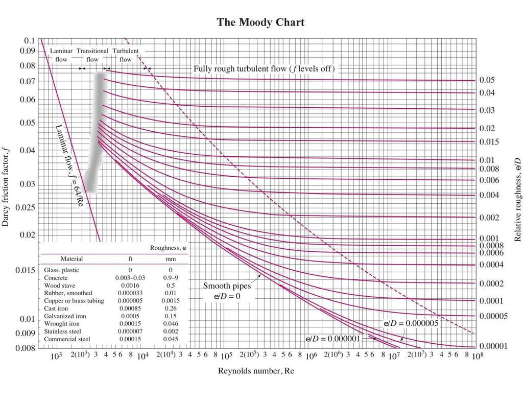
121 Fully Developed Pipe Flow Friction Factor Now go back to equation for hl and substitute f for w fordarcy laminarfriction flow, roughness Our problem is now reduced to solvingbutfor factor f Recall Therefore does not affect the flow unless it is huge Laminar flow: f = 64/Re (exact) Turbulent flow: Use charts or empirical equations (Moody Chart, a famous plot of f vs. Re and /D, See Fig. A-12, p. 898 in text)

122

123 Fully Developed Pipe Flow Friction Factor Moody chart was developed for circular pipes, but can be used for non-circular pipes using hydraulic diameter Colebrook equation is a curve-fit of the data which is convenient for computations (e.g., using EES) Implicit equation for f which can be solved using the root-finding algorithm in EES Both Moody chart and Colebrook equation are accurate to ±15% due to roughness size, experimental error, curve fitting of data, etc.

124 Types of Fluid Flow Problems In design and analysis of piping systems, 3 problem types are encountered 1. Determine p (or hl) given L, D, V (or flow rate) Can be solved directly using Moody chart and Colebrook equation 2. Determine V, given L, D, p 3. Determine D, given L, p, V (or flow rate) Types 2 and 3 are common engineering design problems, i.e., selection of pipe diameters to minimize construction and pumping costs However, iterative approach required since both V and D are in the Reynolds number.

125 Types of Fluid Flow Problems Explicit relations have been developed which eliminate iteration. They are useful for quick, direct calculation, but introduce an additional 2% error

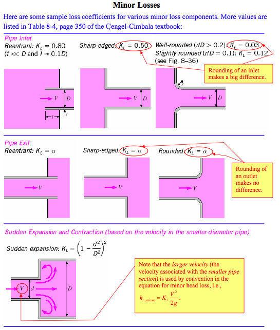
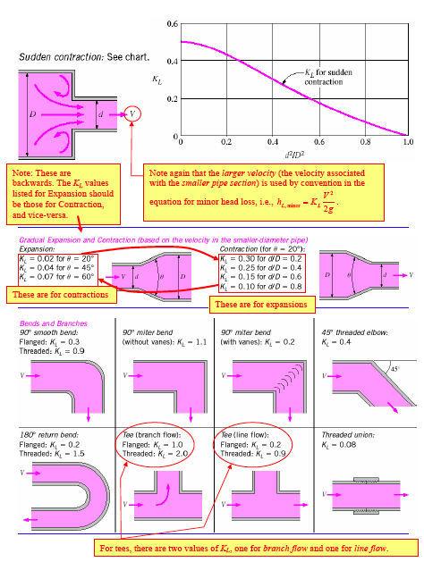
126 Minor Losses Piping systems include fittings, valves, bends, elbows, tees, inlets, exits, enlargements, and contractions. These components interrupt the smooth flow of fluid and cause additional losses because of flow separation and mixing We introduce a relation for the minor losses associated with these components KL is the loss coefficient. Is different for each component. Is assumed to be independent of Re. Typically provided by manufacturer or generic table (e.g., Table 8-4 in text).

127 Minor Losses Total head loss in a system is comprised of major losses (in the pipe sections) and the minor losses (in the components) i pipe sections j components If the piping system has constant diameter

128

129