SUBMITTAL FEASIBILITY STUDY GEOPHYSICAL INVESTIGATION SAN JUAN BASIN SAN JUAN CAPISTRANO, CALIFORNIA. GEOVision Project No

Transcription

1 SUBMITTAL FEASIBILITY STUDY GEOPHYSICAL INVESTIGATION SAN JUAN BASIN SAN JUAN CAPISTRANO, CALIFORNIA GEOVision Project No Prepared for Santa Margarita Water District Antonio Parkway Rancho Santa Margarita, CA (949) Prepared by GEOVision Geophysical Services 1124 Olympic Drive Corona, CA (951) Report rev a March 6, 2015

2 TABLE OF CONTENTS 1 INTRODUCTION ACTIVE AND PASSIVE SURFACE WAVE INVESTIGATION METHODOLOGY EQUIPMENT AND FIELD PROCEDURES Survey Control Active and Passive Seismic Surface Wave Survey DATA PROCESSING SEISMIC REFRACTION INVESTIGATION METHODOLOGY EQUIPMENT AND FIELD PROCEDURES Survey Control Seismic Refraction Survey DATA PROCESSING Tomographic Analysis Technique ELECTRICAL RESISTIVITY INVESTIGATION METHODOLOGY EQUIPMENT AND FIELD PROCEDURES Survey Control Electrical Resistivity Survey DATA PROCESSING TIME-DOMAIN ELECTROMAGNETIC INVESTIGATION METHODOLOGY EQUIPMENT AND FIELD PROCEDURES Survey Control Time-Domain Electromagnetic Survey DATA PROCESSING RESULTS CONCLUSIONS CERTIFICATION Report rev a i March 6, 2015

3 LIST OF TABLES TABLE 1 GEOPHYSICAL TESTING LOCATIONS TABLE 2 S-WAVE VELOCITY MODEL FOR LOCATION 1 TABLE 3 S-WAVE VELOCITY MODEL FOR LOCATION 2 LIST OF FIGURES FIGURE 1 SITE LOCATIONS MAP FIGURE 2 SITE MAP LOCATION 1 FIGURE 3 SITE MAP LOCATION 2 FIGURE 4 SITE MAP LOCATION 3 FIGURE 5 FIGURE 6 FIGURE 7 FIGURE 8 FIGURE 9 FIGURE 10 FIGURE 11 FIGURE 12 FIGURE 13 LINE S-1 S-WAVE REFRACTION MODEL LINE S-2 P-WAVE REFRACTION MODEL VELOCITY MODEL FOR ACTIVE (LINE S-2) AND PASSIVE (ARRAY S-3) SURFACE WAVE ARRAYS LINE S-4 P-WAVE REFRACTION MODEL VELOCITY MODEL FOR ACTIVE (LINE S-4) SURFACE WAVE ARRAY LINE R-1 ELECTRICAL RESISTIVITY MODEL TIME-DOMAIN ELECTROMAGNETIC SOUNDING, 1-D RESISTIVITY MODEL, LOCATION 1 LINE R-2 ELECTRICAL RESISTIVITY MODEL TIME-DOMAIN ELECTROMAGNETIC SOUNDING, 1-D RESISTIVITY MODEL, LOCATION 3 APPENDICES APPENDIX A ACTIVE AND PASSIVE SURFACE WAVE TECHNIQUES SEISMIC REFRACTION METHOD ELECTRICAL RESISTIVITY METHOD TIME-DOMAIN ELECTROMAGNETIC METHOD Report rev a ii March 6, 2015

4 1 INTRODUCTION A geophysical investigation was conducted from February 9 to 12, 2015 at three (3) small areas (Locations 1, 2 and 3) in the San Juan Basin in San Juan Capistrano, California. The objective of the investigation was to determine the effectiveness of several geophysical techniques to map geologic/hydrologic features such as the contact between unconsolidated sediments and the Capistrano Formation, lateral variation in the composition of the sediments (e.g. sand versus clay units) and potential salt-water intrusion in the coastal segment of the basin. Five (5) geophysical methods were evaluated during this investigation: active and passive surface waves, S-wave seismic refraction, electrical resistivity imaging (ERI) and time-domain electromagnetic (TDEM). P-wave seismic refraction models were also developed from the active surface wave field data. Locations 1, 2 and 3 are shown on the Figure 1 Site Locations Map. Site maps for Locations 1, 2 and 3 are shown on Figures 2, 3 and 4, respectively. The active and passive seismic surface wave, S-wave seismic refraction, ERI and TDEM techniques were evaluated at Location 1. The active and passive surface wave and S-wave seismic refraction techniques were applied to determine if they could be effectively utilized to map the top of the Capistrano Formation. The ERI technique was used at Location 1 to determine whether the technique may be effective at mapping the lateral variability of sediments overlying the Capistrano Formation. The TDEM method was applied to determine if it would be effective at mapping subsurface electrical structure in areas with insufficient space for ERI. The active seismic surface wave method was used at Location 2, located on probable Capistrano Formation sediments, to better constrain the seismic velocity of the Capistrano Formation. The ERI and TDEM methods were used at Location 3 to determine if there was a significant decrease in electrical resistivity associated with higher salinity groundwater relative to inland areas of the basin. The approximate locations of each geophysical profile/sounding, as well as, the sensor separations for applicable methods are provided in Table 1. The following sections include a discussion of geophysical methodology, equipment and field procedures, data processing, interpretation of the geophysical data and conclusions. Report rev a 2 March 6, 2015

5 2 ACTIVE AND PASSIVE SURFACE WAVE INVESTIGATION 2.1 METHODOLOGY A discussion of active and passive surface wave methods is provided in the technical note included as Appendix A. The active surface wave technique used includes the multi-channel array surface wave (MASW) method. Passive surface wave technique used includes the array microtremor method. The basis of surface wave methods is the dispersive characteristic of Rayleigh waves when propagating in a layered medium. The phase velocity, V R, depends primarily on the material properties (V S, mass density and Poisson s ratio or compression wave velocity) over a depth of approximately one wavelength. Waves of different wavelengths,, (or frequencies, f) sample different depths. As a result of the variance in the shear stiffness of the layers, waves with different wavelengths travel at different phase velocities; hence, dispersion. A surface wave dispersion curve, or dispersion curve for short, is the variation of V R with or f. The MASW methods are in-situ seismic methods for determining shear wave velocity (V S ) profiles. Surface wave techniques are non-invasive and non-destructive, with all testing performed on the ground surface at strain levels in the soil in the elastic range (< 0.001%). MASW testing consists of collecting multi-channel seismic data in the field and applying a wavefield transform to obtain the dispersion curve and data modeling. Ground motions are recorded by 24 or more geophones typically spaced 1 to 3 m apart and aligned in a linear array and connected to a seismograph. A wavefield transform, such as the f-k, τ-p or phase shift transform, is applied to the time history data to isolate the surface wave dispersion curve. The array microtremor technique uses 4 to 48 receivers aligned in a 2-dimensional array. Triangle, circle, semi-circle and L shaped arrays are commonly used, although any 2- dimensional arrangement of receivers can be used. Receivers typically consist of 1 to 4.5 Hz geophones. The triangle array, which consists of several embedded equilateral triangles, is often used as it provides good results with a relatively small number of geophones. With this array the outer side of the triangle should be at least equal to the desired depth of investigation. The L array is useful at sites located at the corner of perpendicular intersecting streets. Typically 20, or more, 30-second noise records are acquired for analysis. The surface wave dispersion curve is estimated using the extended spatial autocorrelation (ESAC) technique The dispersion curves generated from the active and passive surface wave soundings are generally combined and modeled using an iterative, inverse modeling routine where a V S profile is found whose calculated dispersion curve is a close fit to the field data. The theoretical model used to interpret the dispersion assumes horizontally layered, laterally invariant, homogeneous-isotropic material. Although these conditions are seldom strictly met at a site, the results of active and/or passive surface wave testing provide a good global estimate of the material properties along the array. The results may be more representative of the site than a borehole point estimate. Report rev a 3 March 6, 2015

6 2.2 EQUIPMENT AND FIELD PROCEDURES Survey Control The active surface wave soundings were established by GEOVision in Locations 1 and 2. A passive surface wave sounding was established by GEOVision in Location 1. The soundings were placed as near as feasible to existing water wells, if present, in each location. Geophone locations for the seismic soundings were marked using a 300 ft tape measure. The Sokkia C300 auto level was used to measure relative elevations along the active soundings to allow the use of P-wave refraction processing as well. The relative elevation survey was tied to real-world, approximate elevation using a Trimble ProXRS GPS system with OmniSTAR submeter differential corrections to collected points at the ends of the line. All elevation data were reduced in a spread sheet. The position of each sounding for Locations 1 and 2 are shown on Figures 2 and 3, respectively. The GPS locations of each sounding s center point and sensor separation are summarized in Table Active and Passive Seismic Surface Wave Survey Active surface wave data were acquired using the MASW technique. Passive surface wave data were acquired using the array microtremor method. A typical MASW field layout is shown in Appendix A. MASW equipment used during this investigation consisted of two Geometrics Geode signal enhancement seismographs, 4.5 Hz vertical geophones, seismic cable with 10-foot takeouts, a 4 lb hammer, a 10 lb sledgehammer, a 20 lb sledgehammer and an aluminum plate. MASW data were acquired along a linear array of 48 geophones spaced 5 ft apart. Shot points were located 5, 20, 40, 75 and 100 ft from the end geophone locations and multiple shot points were located in the interior of the array. The 4 lb hammer and 10 lb sledgehammer were used for the 5 ft offset source locations and the center shot. The 20 lb sledgehammer was used at the interior offset source locations. The AWD was used for the 20 ft and greater offset locations. Data from the impact sources were averaged 10 times to improve the signal-to-noise ratio. MASW data was acquired in a manner to also allow P-wave seismic refraction analysis of the field data. Photographs of typical MASW equipment are presented in Appendix A. All field data were saved to hard disk and documented on field data acquisition forms. Array microtremor measurements were made along an L shaped array of 48, 4.5 Hz geophones with a 14 ft geophone spacing along each leg. A typical field layout is shown in Appendix A. The passive surface wave array consisted of two Geometrics Geode signal enhancement seismographs that were used to record forty, 30 sec noise records using a 2 ms sample rate. Data were stored on a laptop computer for later processing and field geometry and associated files names were documented in field data acquisition forms. 2.3 DATA PROCESSING The MASW data were reduced using the software Seismic Pro Surface V6.0 developed by Geogiga using the following steps: Report rev a 4 March 6, 2015

7 Input seismic record into software. Enter receiver spacing, geometry and wavelength restrictions, as necessary. Apply wavefield transform to seismic record to convert the data to phase velocity frequency space. Identify and pick dispersion curve. Repeat for all shot records and merge dispersion curves. Convert dispersion curves to WinSASW format for modeling. The array microtremor data were reduced using the software PICKWIN95 developed by Oyo Corporation using the following steps: Input all seismic records into software. Enter receiver spacing, geometry and wavelength restrictions, as necessary. Calculate the spatial autocorrelation (SPAC) coefficients for each seismic record and average. For each frequency calculate the degree of fit of a first-order Bessel function to the SPAC coefficients for a multitude of phase velocities. Identify and pick dispersion curve as the best fit of the Bessel function for each frequency. Convert dispersion curves to required format for particular modeling software utilized. The surface wave dispersion curves from the active and/or passive surface wave data were used for modeling. An iterative inverse modeling process was used to generate an S-wave velocity model for the sounding. During this process an initial velocity model was generated based on general characteristics of the dispersion curve. The theoretical dispersion curve was then generated using the fundamental mode Rayleigh wave dispersion assumption and compared to the field dispersion curve. Adjustments were then automatically made to the thickness and velocities of each layer and the process repeated until an acceptable fit to the field data was obtained. Data inputs into the modeling software included layer thickness, S-wave velocity, P-wave velocity and mass density. P-wave velocity and mass density only have a very small influence (i.e. less than 10%) on the S-wave velocity model generated from a surface wave dispersion curve. However, realistic assumptions for P-wave velocity, which is impacted by the location of the bedrock, and mass density will slightly improve the accuracy of the S-wave velocity model. Constant mass density values of 112 to 131 lb/ft 3 were used during data modeling with density increasing with V S. Variation in mass density has a negligible effect on surface wave dispersion within the normal range encountered in geotechnical engineering. During data modeling, the compression wave velocity, V P, of unsaturated soils was estimated using a Poisson s ratio, v, of either 0.30 or 0.35 and the relationship: V P = V S [(2(1-v))/(1-2v)] 0.5 Below the saturated zone, estimated at a depth of 40 ft from P-wave refraction data, V P was set to between 5,000 and 6,500 ft/s and increased with depth and V S. Report rev a 5 March 6, 2015

8 3 SEISMIC REFRACTION INVESTIGATION 3.1 METHODOLOGY When conducting a seismic survey, acoustic energy is input to the subsurface by an energy source such as a sledgehammer or weight drop impacting a metallic plate, vibratory source or explosive charge. The acoustic waves propagate into the subsurface at a velocity dependent upon the elastic properties of the material through which they travel. When the waves reach an interface where the density or velocity changes significantly, a portion of the energy is reflected back to the surface, and the remainder is transmitted into the lower layer. Where the velocity of the lower layer is higher than that of the upper layer, a portion of the energy is also critically refracted along the interface. Critically refracted waves travel along the interface at the velocity of the lower layer and continually refract energy back to surface. Receivers (geophones) laid out in linear array on the surface record the incoming refracted and reflected waves. The seismic refraction method involves analysis of the travel times of the first energy to arrive at the geophones. These first arrivals are from either the direct wave (at geophones close to the source), or critically refracted waves (at geophones further from the source). Analysis of seismic refraction data depends upon the complexity of the subsurface velocity structure. If the subsurface target is planar in nature, then the slope intercept method can be used to model multiple horizontal or dipping planar layers. A minimum of one end shot is required to model horizontal layers and reverse end shots are required to model dipping planar layers. If the subsurface target is undulating (i.e., bedrock valley), then layer-based analysis routines such as the generalized reciprocal method, delay time method, time-term method, plus-minus method and wavefront method are required to model subsurface velocity structure. These methods generally require a minimum of 5 shot points per spread (end shots, off-end shots and a center shot). If subsurface velocity structure is complex and cannot be adequately modeled using layerbased modeling techniques (i.e., complex weathering profile in bedrock, numerous lateral velocity variations), then Monte Carlo or tomographic inversion techniques are required to model the seismic refraction data. These techniques require a high shot density (typically every 2 to 4 stations/geophones). Generally these techniques cannot take advantage of off-end shots to extend depth of investigation, so longer profiles are required. Errors in seismic refraction models can be caused by velocity inversions, hidden layers, or lateral velocity variations. At sites with steeply dipping or highly irregular bedrock surfaces, out of plane refractions (refractions from structures to the side of the line rather than from beneath the line) may severely complicate modeling. A velocity inversion is a geologic layer with a lower seismic velocity than an overlying layer. Critical refraction does not occur along such a layer because velocity has to increase with depth for critical refraction to occur. This type of layer, therefore, cannot be recognized or modeled, and depths to underlying layers would be overestimated. A hidden layer is a layer with a velocity increase, but of sufficiently small thickness relative to the velocities of overlying and underlying layers, that refracted arrivals do not arrive at the geophones before those from the deeper, higher velocity layer. Because the seismic refraction method generally only involves the interpretation of first arrivals, a hidden layer cannot be recognized or modeled, and depths to underlying layers would be underestimated. A subsurface velocity structure that increases as a function of depth rather than as discrete layers will also cause depths to subsurface refractors to be underestimated, in a Report rev a 6 March 6, 2015

9 manner very similar to that of the hidden layer problem. Lateral velocity variations that are not adequately addressed in the seismic models will also lead to depth errors. Tomographic imaging techniques can often resolve the complex velocity structures associated with hidden layers, velocity gradients and lateral velocity variations. However, in the event of an abrupt increase in velocity at a geologic horizon, the velocity model generated using tomographic inversion routines will smooth the horizon with velocity being underestimated at the interface and possibly overestimated at depth. 3.2 EQUIPMENT AND FIELD PROCEDURES Survey Control The S-wave seismic refraction line was established by GEOVision in Location 1. The line was placed as near as feasible to existing water well in Location 2. Geophone locations for the S- wave refraction line were marked using a 300 ft tape measure. The Sokkia C300 auto level was used to measure relative elevations along the line. The relative elevation survey was tied to realworld, approximate elevation using a Trimble ProXRS GPS system with OmniSTAR submeter differential corrections to collected points at the ends of the line. All elevation data were reduced in a spread sheet. The position of the S-wave seismic refraction line at Location 1 is shown on Figure 2. The GPS location of the line, the sensor separation and total line length are summarized in Table 1. P-wave seismic refraction data were gathered concurrently with the active surface wave arrays. Details on the active surface wave arrays are found in Section Seismic Refraction Survey The seismic data acquisition system used for the S-wave seismic refraction consisted of two 24- channel Geometrics Geode signal enhancement seismographs combined to form a 48-channel system and a laptop computer running Geometrics Seismodule Controller Software. Other seismic equipment utilized during this investigation consisted of 4.5 Hz horizontal geophones, seismic cable, trigger extension cables, sledgehammers and striking planks. The line consisted of 48 geophones spaced 10 feet apart for a line length of 470 ft. Fifteen (15) shot point locations were occupied: near end shots at geophones 1 and 48, multiple off-end shots and interior shots at regular intervals between every sixth station. For each shot location a horizontal plank or plate was aligned with the strike edges aligned perpendicular to the line. The horizontal plank or plate was then struck by a sledgehammer on side for the shot. This process was repeated on the other side of the horizontal plank or plate to gather reverse polarity information for each shot. A 10- or 20-lb sledgehammer was used as the energy source for each shot point. A hammer switch attached to the hammer and coupled to a trigger extension cable was used to trigger the seismograph upon impact. The final seismic record at each shot point was the result of stacking 7 to 10 shots to increase the signal to noise ratio. All seismic records were stored on a laptop computer. Data files were named with the sequential line, spread and shot number and a.dat extension (i.e. data file 1105.dat is the seismic record from line 1, spread 1, shot 5). Data Report rev a 7 March 6, 2015

10 acquisition parameters, file names and leveling data were recorded in a field log, which is retained in project files. The data acquisition equipment and procedures for the P-wave seismic refraction survey are detailed the active seismic surface wave Section DATA PROCESSING Seismic refraction data were modeled using the tomographic analysis technique with either a smooth starting model or a layered starting model. For P-wave seismic data processing, the layered starting model tomographic analysis technique was used to process the line at Location 2 and smooth starting model tomographic analysis technique was used to model the P-wave refraction data at Location 3. The S-wave refraction data was modeled using the layered starting model tomographic analysis technique. The first step in data processing consisted of picking the arrival time of the first energy received at each geophone (first arrival) for each shot point. For S-wave, the forward and reverse stacks of each shot location were combined to determine the first-arrivals. The cross-over point of the forward and reverse stacks where the energy of the S-wave is first detected is picked for each record. First arrival times were selected using the automatic and manual picking routines in the software package SeisImager (Oyo Corporation) by a GEOVision geophysicist. First arrival times were picked on all seismic records. First arrival times were saved in an ASCII file containing shot location, geophone locations and associated first arrival time. Relative elevations for each geophone location were calculated from the leveling data using a spreadsheet and converted to approximate elevations using GPS data collected at each end of the line. Data quality was affected by factors such as transient noise and geologic conditions. Attempts were made to minimize transient noise as much as possible by waiting for passing traffic during shots Tomographic Analysis Technique Seismic refraction data were modeled using the tomographic analysis technique available in the SeisImager Plotrefa software package, developed by Oyo Corporation. Refraction tomography techniques are often able to resolve complex velocity structure (e.g. velocity gradients) that can be observed in bedrock weathering profiles, but are not well suited to accurately resolving layered structures. Conversely, layer-based modeling techniques such as the generalized reciprocal method can accurately model layered structure, but are not able to accurately model the velocity gradients that can be observed in weathered bedrock. Tomographic inversion techniques will model a smooth velocity gradient even if a sharp velocity boundary exists. The use of layer-based starting models for tomographic inversion will generally sharpen the contact between geologic units with large velocity variation, if present. The layerbased tomographic inversions were used to obtain the expected, abrupt velocity contacts present in the geologic section while also modeling the slight velocity gradients that may be present in the sections. Report rev a 8 March 6, 2015

11 The tomographic inversion was conducted as outlined in the following steps. The first arrival and elevation data were loaded into the software package and a 20 layer initial model was defined with velocity smoothly increasing with depth. The velocity range in the initial model was based on the general characteristics of the travel time data. For the layer-based starting models, layers were assigned in the travel time data and an initial time-term starting model was generated. The time-term model was used as the initial model for the tomographic routines. The velocity models were extended to permit the use of off-end shot points during the inversion with the goal of improving the accuracy of the seismic refraction models near the ends of the lines. A minimum of 20 iterations of non-linear raypath inversion were then implemented to improve the fits of the travel time curves to near-surface sediments/rock. Final tomographic velocity models for each seismic line were exported as ASCII files and imported into the Geosoft Oasis montaj v8 mapping system where the velocity models were gridded, contoured and annotated for presentation. Report rev a 9 March 6, 2015

12 4 ELECTRICAL RESISTIVITY INVESTIGATION 4.1 METHODOLOGY Electrical resistivity imaging (ERI) involves the measurement of the apparent resistivity of subsurface soil and rock as a function of depth and/or position. The resistivity of soils and rock is a complicated function of porosity, permeability, ionic content of the pore fluids and clay mineralization. To conduct an electrical resistivity survey an electrical current is applied to a pair of current electrodes and the potential difference (voltage) is measured between one or more pairs of potential electrodes. For a 2-D resistivity survey, the current and potential electrodes are generally arranged in a linear array. Common array types include the pole-pole, pole-dipole, dipole-dipole, Schlumberger and Wenner arrays. Measured voltages are used to calculate the apparent resistivity of the subsurface. The apparent resistivity is the bulk average of all soils and rock influencing the applied current. It is calculated by dividing the measured potential difference by the input current and multiplying by a geometric factor specific to the array being used, as well as electrode spacing. Apparent resistivity is typically run through an inverse modeling algorithm to generate a geoelectric section of the subsurface directly beneath the profile. In general, for 2-D electrical resistivity surveys, resolution and depth of investigation are inversely proportional. High resolution is typically obtained by using relatively small electrode spacing. However, using small electrode spacing reduces investigation depth. Conversely, large electrode separation will typically provide greater depth of investigation, but sacrifices resolution. 4.2 EQUIPMENT AND FIELD PROCEDURES Survey Control Each ERI line was established by GEOVision in Locations 1 and 3. The lines were placed as near as feasible to existing water wells in each location. The line was adjusted to maximize data coverage in the target area. Electrode locations for the ERI lines were marked using a 300 ft tape measure. The Sokkia C300 auto level was used to measure relative elevations along the line. The relative elevation survey was tied to real-world approximate elevation using a Trimble ProXRS GPS system with OmniSTAR submeter differential corrections to collected points at the ends of the line. All elevation data were reduced in a spread sheet. The position of each ERI line for Locations 1 and 3 are shown on Figures 2 and 4, respectively. The ERI GPS locations, sensor separation and total line lengths are summarized in Table Electrical Resistivity Survey 2D electrical resistivity data were acquired along the geophysical traverses using an AGI SuperSting R8/IP 112-electrode system. A 10 or 15 ft electrode spacing was used to allow high resolution imaging of the near surface and a depth of investigation in excess of 150 ft. Additionally, the SuperSting was programmed to acquire data in multiple passes to increase data density and minimize potential cultural noise. A salt water solution was added to electrode Report rev a 10 March 6, 2015

13 locations staked in surface soil to minimize contact resistance between the electrode stake and the surrounding soil, as necessary. Contact resistance measurements were recorded prior to data acquisition. Electrodes exhibiting abnormally high contact resistance were treated or retreated with saline solution and checked for good contact. ERI data were acquired using both the dipole-dipole and inverse Schlumberger arrays. The SuperSting was programmed with the appropriate acquisition parameters and set to record automatically along the 112 electrode spread. Resistivity data were stored in the internal memory of the SuperSting R8/IP and downloaded to a laptop computer upon completion of the field investigation. Field data files were assigned a name that included profile number and array type. 4.3 DATA PROCESSING Dipole-dipole and inverse Schlumberger data were modeled separately using the program EarthImager 2D v2.4.0 by Advanced Geosciences, Inc. A smooth model inversion algorithm using a finite element mesh with surface topography was selected to generate the 2D earth model of resistivity versus depth/elevation, called a geoelectric section. The starting model for the inversion was based on the average apparent resistivity of the acquired data. Additionally, the dipole-dipole and inverse Schlumberger data were merged before inversion. The combined model can provide the near surface resolution of the inverse Schlumberger array and the depth of the dipole-dipole array. Inversion output was saved as an ASCII format XYZ file containing position, elevation and resistivity. The data were imported into Golden Software, Inc. Surfer for gridding, contouring and final presentation. All files generated during processing are archived. Report rev a 11 March 6, 2015

14 5 TIME-DOMAIN ELECTROMAGNETIC INVESTIGATION 5.1 METHODOLOGY The time-domain electromagnetic (TDEM) instrument used during this investigation consisted of a Geonics EM-47 transmitter, high-frequency receiver coil and a Protem digital receiver. This system is designed to image to a maximum depth of about 100 m, whereas other systems such as the Geonics EM-57 and EM-37 are designed with larger transmitters and lower-frequency coils to image to greater depth. A TDEM system consists of a separate transmitter (Tx) and receiver (Rx) coils. The Tx coil generally consists of a square loop of insulated wire laid on the surface. The Rx coil is generally placed in the center of the Tx loop (central loop sounding) but map be placed outside the Tx loop (offset loop sounding). The EM-47 transmitter operates at three user-selectable repetition frequencies of 285, 75, and 30 Hz and is synchronized to the Protem receiver using a reference cable. Depending on the required resolution and depth of investigation, the dimensions of the transmitter loop may be changed. In the central loop sounding mode, 30 by 30 m to 100 by 100 m Tx loops can be used with the EM-47 transmitter. Larger loops allow deeper depths of investigation and reduced noise level, at some loss of resolution. The 100-watt battery-powered EM-47 transmitter is used to drive a modified square-wave current through the Tx loop. One period of the transmitted waveform (33.3 milliseconds for the 30 Hz repetition frequency) consists of two current-on (time-on) and two current-off (time-off) cycles. At the end of the first time-on cycle, the current is abruptly switched off for a quarter period using a rapid linear ramp. During the following time-on cycle, the current flows in the opposite direction. The abrupt termination of the current induces a short-duration voltage pulse in the ground in accordance with Faraday s Law of Induction. This voltage pulse gives rise to a current loop in the ground in the immediate vicinity of the Tx loop. The location of the maximum current intensity diffuses downward and outward with time, thereby providing information on the electrical properties of successively deeper materials. The diffusing current system produces a time-varying secondary magnetic field, which is measured as a voltage induced in the receiver coil. The Geonics PROTEM receiver measures the decaying secondary magnetic field at 20 logarithmically-spaced gates during the transmitter time-off cycle only. Many hundreds to thousands of measurements are stacked to improve data quality. The measurements are converted to apparent resistivity by calculating the resistivity of a uniform half-space that would give rise to the measured voltage. 5.2 EQUIPMENT AND FIELD PROCEDURES Survey Control Each TDEM sounding was established by GEOVision in Locations 1 and 3. One sounding was collected in each location for a total of two (2) soundings. Each sounding was placed in an area free of surface metal near the end of the each ERI line. Using 300 ft tape measures, the corners of each loop were established using approximately 40 m on a side. These locations were staked and used to pull the transmitter wire loops to the appropriate dimensions for the soundings. The Report rev a 12 March 6, 2015

15 receiver loop was placed 10 m on the outside of the edge of the transmitter wire loop. A Trimble ProXRS GPS system with OmniSTAR submeter differential corrections was used to collect the approximate center point of each sounding. The position of each TDEM sounding for Locations 1 and 3 are shown on Figures 2 and 4, respectively. The GPS locations for the center points of each TDEM sounding are presented in Table Time-Domain Electromagnetic Survey A Geonics EM47 transmitter (Tx), high-frequency receiver coil and a Protem digital receiver (Rx) were used to conduct TDEM soundings. The TDEM soundings were conducted in the offset-loop sounding mode where the receiver coil is placed outside of the transmitter loop during data recording. At each sounding location a transmitter loop consisting of insulated 12-gauge copper wire was placed on the ground in a square loop with roughly 40 m sides. The receiver coil was placed 10 m away from the outside the edge of the Tx loop. The receiver coil was connected to the Protem Receiver and a reference cable between the transmitter and receiver synchronized the system. The 100-watt battery-powered EM-47 transmitter, placed at a corner of each wire-loop, was used to drive current pulses through the wire. The EM47 transmitter was operated at repetition frequencies of 285, 75 and 30 Hz. Generally, transmitter currents of 1 to 3 amperes were used for the 285 to 30 Hz repetition rates, respectively. The current pulses induced eddy current flow in the subsurface. The receiver coil positioned in the center of the wire-loop is used to record the decay of the secondary magnetic field due to the eddy currents induced in the subsurface. The Geonics Protem receiver measured the decaying secondary magnetic field at 20 logarithmicallyspaced gates during the transmitter time-off cycle only. The data acquired at each sounding center consisted of measurements at several different receiver gain settings for the two transmitter frequencies. This was accomplished in order to assure data quality and to obtain data over the largest possible time interval. Additionally, hundreds of measurements were stacked at each location to improve the signal to noise ratio. The measurements were converted to apparent resistivity by calculating the resistivity of a uniform half-space that would give rise to the measured voltage. The data from each sounding were stored in solid-state memory in the receiver and transferred at the end of the day to a computer for processing. 5.3 DATA PROCESSING The TDEM field data collected for the two soundings were transferred from the Geonics PROTEM receiver to a PC for editing and processing. All processing and modeling of the TDEM data was performed with the software package TEMIX XL (Interpex Ltd.). The initial step in processing was to input all of the soundings into the program. During data input the measurements made at the various amplifier gains and frequencies for each sounding were combined to produce one voltage decay curve (transient). Next, the data were transformed into apparent resistivity versus recorded time gate. The apparent resistivity curve was modeled by inversion to obtain a one-dimensional (1-D) geoelectric section that most closely matches the observed decay curve. Two types of inversion routines can be utilized: a 1D layered model inversion and a 1D smooth model inversion. The TEMIX XL 1D layered model inversion Report rev a 13 March 6, 2015

16 routine requires an initial model of the geoelectric section, which includes the number of layers and the thickness and resistivity of each of the layers. The inversion program then adjusts these parameters so that the model curve converges to best fit the curve formed by the field data. The inversion program does not change the number of layers within the model curve, but allows all other parameters to change freely or they can optionally be made constant. To determine the influence and best fit of the number of layers on the solution, separate inversions with different numbers of layers are run. The model with the fewest number of layers, which best fits the data is used in the final interpretation. The TEMIX XL smooth model inversion routine requires the user to specify the number of layers (typically 10 to 20), the thickness of the first layer and the depth of the final layer. Optionally, the program can calculate a default thickness of the first layer and depth of the final layer. The program increases layer thickness with depth to account for loss of vertical resolution with depth. Smooth model inversions were not conducted during this investigation. The interpreted geoelectric section derived from each TDEM sounding is not unique. The magnitude of each individual layer resistivity and thickness can normally be varied within a limited range with no significant change to the fit of the geoelectric model of the field data. This variation in fit parameters is termed equivalence and is a problem faced by most surface geophysical techniques. An equivalence analysis was performed for each of the TDEM soundings to estimate a range of models that fit the field observations almost as well as the best fit model. Another form of analyzing equivalence is in the total number of layers used in the inversion model. In the TEMIX XL program, the interpreter sets a fixed number of layers. During the inversion process, the program adjusts the layer resistivity and thickness so the model best fits the field data. Generally, a minimum number of layers are used in the modeling program. This is determined by increasing the number of layers in the model, until additional layers do not significantly improve the fit of the model to the field data. Inversion models with three to four layers were generally used for the TDEM data collected during this investigation. Report rev a 14 March 6, 2015

17 6 RESULTS The S-wave seismic refraction, active and passive surface wave, ERI and TDEM methods were evaluated at Location 1 (Figure 2). The S-wave seismic refraction model for Line S-1, developed using a tomographic inversion routine with a layered starting model, is presented as Figure 5. This technique was applied to determine if it may be effective at mapping the top of the Capistrano Formation. There is an abrupt increase in S-wave velocity to over 1,500 ft/s at an average depth of about 105 ft, which is likely associated with the top of the Capistrano Formation. Active surface wave data were acquired along Line S-2 using the MASW technique and passive surface wave data were acquired using the L-shaped array S-3 (Figure 2). A P-wave seismic refraction model was also developed for the MASW data acquired along Line S-2, primarily to anchor the depth to the saturated zone during modeling of the surface wave data. The P-wave refraction model for Line S-2, developed using a tomographic inversion routine with a layered starting model, is presented as Figure 6 and indicates that the saturated zone is located at an average depth of about 35 to 40 ft. P-wave velocity increases to greater than 4,800 ft/s once sediments become over 99% saturated. Since there may not be much variation in P-wave velocity between saturated alluvium and Capistrano Formation, the P-wave refraction technique was not considered for mapping the Capistrano Formation. S-wave velocity, however, is not affected by the presence of water in pore spaces. An S-wave velocity model developed from the combined active and passive surface wave data from Line S-2 and Array S-3, respectively, is presented as Figure 7 and Table 2. The depth of investigation of active surface wave techniques is generally limited to about 100 ft when using cost effective energy sources, but can be extended by the addition of passive surface wave data. Although Line S-2 and Array S-3 are not coincident, there is good agreement in the surface wave dispersion data in the overlapping wavelength range and, therefore, the datasets could be combined for modeling. There is an abrupt increase in S-wave velocity to about 1,550 ft/s at a depth of 105 ft, which is interpreted as being the contact between alluvium and Capistrano Formation. S-wave velocity in the alluvium gradually increases with depth ranging from about 700 ft/s near the surface to 1,050 ft/s at a depth of 70 ft. To better constrain the expected S-wave velocity range of the Capistrano Formation, active surface wave (MASW) and P-wave seismic refraction data was acquired along Line S-4, located on mapped Capistrano Formation at Location 2 (Figure 3). The P-wave seismic refraction model for Line S-4 is presented as Figure 8. There were indications of thin high velocity layers in the seismic data and, therefore, the P-wave velocity model may overestimate seismic velocities because the seismic refraction method cannot image velocity inversions. The active surface wave data is much less sensitive to thin, high velocity layers and generally yields more accurate average velocity structure, even though the thin, high velocity layers may be too thin to image. The S-wave velocity model resulting from the active surface wave data of Line S-4 is presented as Figure 9 and Table 3. S-wave velocities are generally lower than expected with about 30 ft of sediments and residual soil/intensely weathered Capistrano Formation having S-wave velocity between about 585 and 910 ft/s. Below 30 ft S-wave velocity increases to about 1,130 ft/s in what is likely weathered Capistrano Formation or a less consolidated member of the Capistrano Formation than that encountered beneath Line S-2. S-wave velocity increases to about 1,875 ft/s at a depth of about 100 ft in what is interpreted as competent or a more consolidated member of the Capistrano Formation. Report rev a 15 March 6, 2015

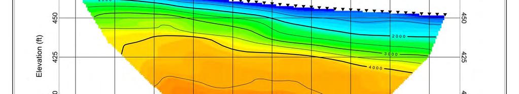
18 The ERI model for Line R-1 is presented as Figure 10 and presents the variation of electrical resistivity with distance and depth along the profile. The ERI data is modeled using a smooth model inversion routine; therefore, the model will show smoothly varying resistivity even if abrupt layer contacts are present. For the purpose of discussion, dashed lines are shown on Figure 10 at depths of about 40 ft and 105 ft referencing the approximate top of the saturated zone and Capistrano Formation as identified from S-wave refraction and active/passive surface wave data. In the unsaturated zone, high resistivity is typically associated with sands and gravels and the low resistivity zones associated with clays. In the saturated zone, resistivity decreases as the total dissolved solids (TDS) content of the pore water increases and as the clay content increases. The resistivity model for Line R-1 (Figure 10) has a thin, intermediate resistivity layer (typically 50 to 100 ohm-m) at the surface probably associated with finer-grained fill soils underlain by a highly resistive unit (typically greater than 400 ohm-m), likely associated with unsaturated sands. Resistivity generally decreases below 40 ft where the sediments become saturated and decreases again below 105 ft in the Capistrano Formation. The resistivity of the saturated alluvium and Capistrano Formation are generally in the 30 to 100 and 10 to 50 ohm-m ranges, respectively. The primary purpose of ERI imaging in the San Juan Basin is to map lateral variability of sediments in the alluvium (i.e. differentiate sediments that are primarily sand versus those that are finer-grained). In the unsaturated zone (i.e. above a depth of about 40 ft) resistivity is on average slightly lower northeast of a position of 750 ft, but still very resistive, indicating a possible slight fining of the sediments (i.e. greater silt content and minor amounts of clay). In the saturated sediments between depths of about 40 and 105 ft there are several areas with variable resistivity. These include high resistivity zones centered at positions of 325 and 575 ft, that could be associated with coarser-grained sand and gravel and/or lower TDS pore water, and lower resistivity sediments between 425 and 525 ft that could be associated with saturated clays and/or higher TDS pore water. In the Capistrano Formation below a depth of about 105 ft, resistivity is slightly higher in the southwestern portion of the profile indicating that the formation maybe slightly coarser grained (i.e. more silt content). A 1-D three layer resistivity model for the single TDEM sounding conducted in Location 1 is presented as Figure 11. The model is generally consistent with the ERI model, showing resistivity decreasing with depth as the sediments first becomes saturated and again the finegrained Capistrano Formation is encountered. The uppermost layer in the TDEM model has a resistivity of 305 ohm-m and thickness of 14 m (46 ft) and is primarily associated with coarsegrained unsaturated sediments. Equivalence analysis indicates that the resistivity of this layer is not well constrained and the thickness may vary from 10 to 20%. The second layer has a resistivity of 6 ohm-m and thickness of 20 m (66 ft) and is associated with saturated alluvium. Equivalence analysis indicates that the resistivity of this layer is relatively well constrained but the thickness may vary by 10%, or more. The resistivity of this layer is much lower than estimated from the ERI data and review of available borehole data is necessary to determine which data set is yielding more accurate resistivity. The lowest layer, located at a depth of about 34 m (112 ft) has a resistivity of 1 ohm-m and is likely associated with the Capistrano Formation. The resistivity of this layer is also much lower than that estimated from the ERI data. The ERI and TDEM methods were evaluated at Location 3 (Figure 4), which is located on the coastal side of the San Juan Basin. The primary purpose of the geophysical survey in this area was to determine if electrical and electromagnetic methods had application in mapping the higher salinity saturated sediments associated with salt water intrusion in this portion of the Report rev a 16 March 6, 2015

19 basin. The ERI model for Line R-2 is presented as Figure 12. The resistivity model indicates that there is a very thin resistive layer of sand, underlain by saturated sediments. The upper 75 to 100 ft of the saturated sediments have resistivity in the 5 to 60 ohm-m range, averaging about 15 to 20 ohm-m. The resistivity of this unit is definitely lower than that observed for saturated sediments beneath Line R-1, indicating the groundwater has higher TDS in this area. Resistivity is much lower at greater depths, typically ranging from about 2 to 10 ohm m due to higher salinity groundwater and/or the presence of the fine-grained Capistrano Formation. The TDEM data acquired at Location 3 had higher noise levels than that acquired at Location 1, possibly due to the reinforced concrete in the walls of the channel and/or electrical noise from nearby power lines. A 1-D three layer resistivity model for the single TDEM sounding conducted in Location 3 is presented as Figure 13. The model is generally consistent with the ERI model, showing resistivity decreasing with depth as the TDS/salinity of the saturated sediments possibly increase and then as the fine-grained Capistrano Formation is encountered. The uppermost layer in the TDEM model has a resistivity of 23 ohm-m and thickness of 14 m (46 ft) and is primarily associated with the uppermost zone of saturated sediments. Equivalence analysis indicates that the resistivity of this layer is not well constrained and the thickness may vary from 10 to 20%. The second layer has a resistivity of 3 ohm-m and thickness of 38 m (125 ft) and is associated with saturated sediments with higher TDS/salinity. Equivalence analysis indicates that the resistivity of this layer is relatively well constrained but that the thickness is poorly constrained. As with the TDEM sounding at Location 1, the resistivity of this layer is much lower than estimated from the ERI data and review of available borehole data is necessary to determine which data set is yielding the more accurate resistivity. The lowest layer, located at a depth of about 52 m (171 ft) has a resistivity of 1 ohm-m and is likely associated with the Capistrano Formation. Equivalence analysis indicates that the resistivity and depth of this layer are not well constrained. The electrical resistivity of the saturated sediments, both in the ERI and TDEM models, are lower than observed at Location 1, indicating that on average the TDS/salinity of the groundwater is higher at Location 3.. Report rev a 17 March 6, 2015

20 7 CONCLUSIONS A geophysical feasibility study was conducted in the San Juan Basin in San Juan Capistrano, California. The objective of the investigation was to determine the most appropriate method(s) to map varying soil type in the alluvial sediments (i.e. areas that are predominantly sand versus areas that are predominantly clay), the top of the Capistrano Formation and possible saltwater intrusion near the mouth of the channel. Three (3) sites were used for testing five (5) geophysical techniques. These sites were designated Locations 1, 2 and 3 (Figure 1). The five (5) geophysical methods that were tested for feasibility include: active and passive seismic surface wave, S-wave seismic refraction, electrical resistivity imaging (ERI), time-domain electromagnetics (TDEM). P-wave seismic refraction analysis was also conducted on seismic data acquired during the active surface wave investigation. The MASW, array microtremor, S- wave seismic refraction, ERI and TDEM methods were tested at Location 1 (Figure 2). The MASW method was tested at Location 2 (Figure 3) and the ERI and TDEM methods were tested at Location 3 (Figure 4). The S-wave seismic refraction model for Line S-1 (Location 1) is presented as Figure 5. The P- wave seismic refraction models for Line S-2 (Location 1) and S-4 (Location 2) are presented as Figures 6 and 8, respectively. The S-wave velocity models resulting from analysis of active and passive surface wave data collected on Line S-2 and array S-3 (Location 1) and MASW data collected along Line S-4 (Location 2) are presented as Figures 7 and 9, respectively. These data sets demonstrate that both the S-wave seismic refraction and active/passive surface wave techniques can be utilized to map the top of the Capistrano Formation. The S-wave seismic refraction technique requires an environment with low noise (i.e. vehicular traffic) and sufficient space for a 470 ft, or longer, profile and can provide 2-D models of velocity structure if data quality is sufficient. The combined active and passive surface wave techniques can image to greater depths with less available space and can be conducted in urban areas (i.e. along sidewalks) but only provide a 1-D S-wave velocity model. Both techniques should be capable of estimating the depth of the Capistrano Formation with a typical accuracy of about 10% of depth. The Capistrano Formation within the San Juan Basin is expected to be relatively unweathered, as weathered material has likely been eroded away, with S-wave velocity exceeding 1,500 ft/s. Near the edges of the basin S-wave velocity of the Capistrano Formation may be as low as 1,150 ft/s if weathered material remains in place. The MASW profile conducted at Location 2 which is located on an on an area mapped as Capistrano Formation, indicates that significant weathered and/or lower velocity rock units may occur in some of the hills bounding the basin. Because density is loosely related to seismic velocity (i.e. density generally increases with seismic velocity), the presence of residual soil deposits and weathered Capistrano Formation in the hills bounding the basin, may severely limit the effectiveness of the gravity technique at mapping the geometry of the basin. The electrical resistivity models for ERI Line R-1 and the TDEM sounding conducted at Location 1 are presented as Figures 10 and 11, respectively. These models demonstrate that there is generally a resistivity decrease associated with both the saturated zone and the top of the Capistrano Formation. The P-wave refraction technique is likely better suited to mapping the top of the saturated zone and S-wave velocity techniques (refraction and surface wave) are better suited to mapping the top of the Capistrano Formation. However, the ERI model demonstrates that the ERI method is capable of mapping zones where there is a thicker sequence of coarser- Report rev a 18 March 6, 2015

21 grained sediments, which is important in siting potential groundwater recharge areas and cannot be imaged using seismic techniques. The electrical resistivity models for ERI Line R-2 and the TDEM sounding conducted at Location 3 are presented as Figures 12 and 13, respectively. These models demonstrate that the electrical resistivity of the saturated sediments near the coast is lower than the inland area of Location 1, indicating that the electrical resistivity and/or TDEM methods may have application at the site to map salt water intrusion and other water quality issues. The resistivity method is preferred for mapping lateral variability of resistivity structure in the alluvial sediments but requires profiles with a minimum length of about 750 ft to image to a depth of 150 ft. The TDEM method can image 1-D resistivity structure to this depth with a transmitter loop size as small as 100 to 150 ft, so it is more suited to imaging subsurface electrical structure where there is less space (e.g. small parks, ball fields). However, TDEM is more affected by cultural influences such as electrical lines and metallic surface features. Additionally, the TDEM method is better suited to mapping electrical conductors such as saline water associated with salt water intrusion. Report rev a 19 March 6, 2015

22 8 CERTIFICATION All geophysical data, analysis, interpretations, conclusions, and recommendations in this document have been prepared under the supervision of and reviewed by a GEOVision California Professional Geophysicist. Prepared by Antony J. Martin California Professional Geophysicist P.Gp. 989 GEOVision Geophysical Services March 6, 2015 Date This geophysical investigation was conducted under the supervision of a California Professional Geophysicist using industry standard methods and equipment. A high degree of professionalism was maintained during the project from the field investigation and data acquisition, through data processing interpretation and reporting. Original field data files, field notes and observations, and other pertinent information are maintained in the project files and are available for the client to review for a period of at least one year. A professional geophysicist s certification of interpreted geophysical conditions comprises a declaration of his/her professional judgment. It does not constitute a warranty or guarantee, expressed or implied, nor does it relieve any other party of its responsibility to abide by contract documents, applicable codes, standards, regulations or ordinances. Report rev a 20 March 6, 2015

23 TABLES

24 Table 1 Geophysical Testing Locations Site Geophysical Sensor Approximate Location Easting (US Feet) Northing (US Feet) Location Method Separation (ft) Elevation (ft) 1 S-Wave Refraction 10 0 ft 6,136,994 2,130, ft 6,137,415 2,131, MASW 5 Center 6,137,208 2,130, Passive L-Array 14 Center 6,137,193 2,131, Electrical Resistivity 0 ft 6,136,707 2,130, Imaging 1110 ft 6,137,659 2,131, TDEM N/A Center 6,137,319 2,130, MASW 5 Center 6,135,909 2,124, Electrical Resistivity 0 ft 6,124,749 2,116, Imaging 1665 ft 6,125,245 2,117, TDEM N/A Center 6,125,301 2,117, Notes: 1. Coordinates taken with a Trimble ProXRS GPS system with OmniSTAR submeter real-time differential corrections 2. Coordinates in CA State Plane, NAD83, Zone VI (0406), US Survey Feet

25 Depth to Top of Layer (ft) Table 2 S-Wave Velocity Model for Location 1 Layer Thickness (ft/s) S-Wave Velocity (ft/s) Inferred P- Wave Velocity (ft/s) Assumed Poisson's Ratio Assumed Density (lb/ft 3 ) , , ,054 5, ,549 6, >45.0 2,150 6, Depth to Top of Layer (ft) Table 3 S-Wave Velocity Model for Location 2 Layer Thickness (ft/s) S-Wave Velocity (ft/s) Inferred P- Wave Velocity (ft/s) Assumed Poisson's Ratio Assumed Density (lb/ft 3 ) , , , ,128 2, >50.0 1,876 3,

26 FIGURES

27 LOCATION 1 LOCATION LOCATION ,500 3,000 4,500 Feet FIGURE 1 SITE LOCATIONS MAP NOTES: 1. California State Plane Coordinate System, NAD 83 Zone VI (0406), US Survey Feet 2. Image Source: Esri, DigitalGlobe, GeoEye, i-cubed, USDA, USGS, AEX, Getmapping, Aerogrid, IGN, IGP, swisstopo, and the GIS User Community p Date: GV Project: Developed by: Drawn by: Approved by: File Name: 3/5/ D Carpenter T Rodriguez A Martin MXD SAN JUAN BASIN FEASABILITY STUDY SITES SAN JUAN CAPISTRANO, CA PREPARED FOR SANTA MARGARITA WATER DISTRICT

28 Array S-3 Line R ' 0' Line S-1 MW-06 0' Line S-2 TDEM!.!. 235' 117.5' 0' 470' Feet Legend!. Center of Time Domain Electromagnetics Array!. Monitoring Well Location Electrical Resistivity Imaging Array Passive Surface Wave Array (L Array) MASW and P-Wave Refraction Line S-Wave Seismic Refraction Line NOTES: 1. California State Plane Coordinate System, NAD 83 Zone VI (0406), US Survey Feet 2. Image Source: Esri, DigitalGlobe, GeoEye, i-cubed, USDA, USGS, AEX, Getmapping, Aerogrid, IGN, IGP, swisstopo, and the GIS User Community 3. Monitoring Well Locations Visually Referenced from Google Earth p Date: GV Project: Developed by: Drawn by: Approved by: File Name: 3/5/ D Carpenter T Rodriguez A Martin MXD FIGURE 2 SITE MAP - LOCATION 1 SAN JUAN BASIN FEASABILITY STUDY SITES SAN JUAN CAPISTRANO, CA PREPARED FOR SANTA MARGARITA WATER DISTRICT

29 Line S-4 235' 117.5' 0' Feet Legend MASW and P-Wave Refraction Line FIGURE 3 SITE MAP - LOCATION 2 NOTES: 1. California State Plane Coordinate System, NAD 83 Zone VI (0406), US Survey Feet 2. Image Source: Esri, DigitalGlobe, GeoEye, i-cubed, USDA, USGS, AEX, Getmapping, Aerogrid, IGN, IGP, swisstopo, and the GIS User Community 3. Monitoring Well Locations Provided by South Coast Water District p Date: GV Project: Developed by: Drawn by: Approved by: File Name: 3/5/ D Carpenter T Rodriguez A Martin MXD SAN JUAN BASIN FEASABILITY STUDY SITES SAN JUAN CAPISTRANO, CA PREPARED FOR SANTA MARGARITA WATER DISTRICT

30 TDEM!. 1665' Line R-2!. MW ' Feet Legend!. Center of Time Domain Electromagnetics Array!. Monitoring Well Location Electrical Resistivity Imaging Array NOTES: 1. California State Plane Coordinate System, NAD 83 Zone VI (0406), US Survey Feet 2. Image Source: Esri, DigitalGlobe, GeoEye, i-cubed, USDA, USGS, AEX, Getmapping, Aerogrid, IGN, IGP, swisstopo, and the GIS User Community 3. Monitoring Well Locations Provided by South Coast Water District p Date: GV Project: Developed by: Drawn by: Approved by: File Name: 3/5/ D Carpenter T Rodriguez A Martin MXD FIGURE 4 SITE MAP - LOCATION 3 SAN JUAN BASIN FEASABILITY STUDY SITES SAN JUAN CAPISTRANO, CA PREPARED FOR SANTA MARGARITA WATER DISTRICT

31

32

33 Comparison of Field, Representative and Inverted Theoretical Dispersion Curve from Active and Passive Surface Wave Arrays 0 50 Depth, ft Alluvium Capistrano Formation Shear Wave Velocity (V S ), ft/s V S Model from Active and Passive Surface Wave Arrays Project No.: Date: MAR. 3, 2015 Drawn By: D. CARPENTER Approved By: A. MARTIN File P:\...Project Files\2015\15027SantaMargarita...\report\Figure7.cdr FIGURE 7 VELOCITY MODEL FOR ACTIVE (LINE S-2) AND PASSIVE (ARRAY S-3) SURFACE WAVE ARRAYS LOCATION 1 SAN JUAN CAPISTRANO, CALIFORNIA PREPARED FOR SANTA MARGARITA WATER DISTRICT

34

35 Comparison of Field, Representative and Inverted Theoretical Dispersion Curve from Active Surface Wave Array Sediments / Residual Soil????? Weathered Capistrano Fm. Depth, ft Competent Capistrano Formation Shear Wave Velocity (V S ), ft/s V S Model from Active Surface Wave Array Project No.: Date: MAR. 3, 2015 Drawn By: D. CARPENTER Approved By: A. MARTIN File P:\...Project Files\2015\15027SantaMargarita...\report\Figure9.cdr FIGURE 9 VELOCITY MODEL FOR ACTIVE (LINE S-4) SURFACE WAVE ARRAY LOCATION 2 SAN JUAN CAPISTRANO, CALIFORNIA PREPARED FOR SANTA MARGARITA WATER DISTRICT

36

37 Field Measurements APPARENT RESISTIVITY (ohm-m) Calculated Response Depth (m x 10) Best Fit Model Equivalence Model TIME (ms) RESISTIVITY (ohm-m) Project No.: Date: MAR 6, 2015 Drawn By: W. DALRYMPLE Approved By: A. MARTIN File P:\...Project Files\2015\15027SantaMargarita...\report\Figure11.cdr FIGURE 11 TIME-DOMAIN ELECTROMAGNETIC SOUNDING 1-D RESISTIVITY MODEL LOCATION 1 SAN JUAN CAPISTRANO, CALIFORNIA PREPARED FOR SANTA MARGARITA WATER DISTRICT

38

39 100 0 Field Measurements Calculated Response 1 APPARENT RESISTIVITY (ohm-m) 10 Depth (m x 10) Best Fit Model Equivalence Model TIME (ms) RESISTIVITY (ohm-m) Project No.: Date: MAR 6, 2015 Drawn By: W. DALRYMPLE Approved By: A. MARTIN File P:\...Project Files\2015\15027SantaMargarita...\report\Figure13.cdr FIGURE 13 TIME-DOMAIN ELECTROMAGNETIC SOUNDING 1-D RESISTIVITY MODEL LOCATION 3 SAN JUAN CAPISTRANO, CALIFORNIA PREPARED FOR SANTA MARGARITA WATER DISTRICT

40 APPENDIX A

41 ACTIVE AND PASSIVE SURFACE WAVE TECHNIQUES Overview Active and passive surface wave techniques are relatively new insitu seismic methods for determining shear wave velocity (V S ) profiles. Testing is performed on the ground surface, allowing for less costly measurements than with traditional borehole methods. The basis of surface wave techniques is the dispersive characteristic of Rayleigh waves when traveling through a layered medium. Rayleigh wave velocity is determined by the material properties (primarily shear wave velocity, but also to a lesser degree compression wave velocity and material density) of the subsurface to a depth of approximately 1 to 2 wavelengths. As shown in the adjacent diagram, longer wavelengths penetrate deeper and their velocity is affected by the material properties at greater depth. Surface wave testing consists of measuring the surface wave dispersion curve at a site and modeling it to obtain the corresponding shear wave velocity profile. λ λ λ λ Active Surface Wave Techniques Active surface wave techniques measure surface waves generated by dynamic sources such as hammers, weight drops, electromechanical shakers, vibroseis and bulldozers. These techniques include the spectral analysis of surface waves (SASW) and multi-channel array surface wave (MASW) methods. Hammer Energy Sources Accelerated Weight Drop Electromechanical Shaker Bulldozer Energy Source 1124 Olympic Drive, Corona, California ph fx

42 The SASW method is optimized for conducting V S depth soundings. A dynamic source is used to generate surface waves of different wavelengths (or frequencies) which are monitored by two or more receivers at known offsets. An expanding receiver spread and optimized source-receiver geometry are used to minimize near field effects, body wave signal and attenuation. A dynamic signal analyzer is typically used to calculate the phase and coherence of the cross spectrum of the time history data collected at a pair of receivers. During data analysis, an interactive masking process is used to discard low quality data and to unwrap the phase spectrum, as shown in the figure below. The dispersion curve (Rayleigh wave phase velocity versus frequency or alternatively wavelength) is calculated from the unwrapped phase spectrum. SASW Setup HP Dynamic Signal Analyzer Masking of Wrapped Phase Spectrum and Resulting Dispersion Curve The MASW field layout is similar to that of the seismic refraction technique. Twenty four, or more, geophones are laid out in a linear array with 1 to 2m spacing and connected to a multi-channel seismograph as shown below. This technique is ideally suited to 2D V S imaging, with data collected in a roll-along manner similar to that of the seismic reflection technique. The source is offset at a predetermined distance from the near geophone usually determined by field testing. The Rayleigh wave dispersion curve is obtained by a wavefield transformation of the seismic record such as the f-k or τ-p transforms. These transforms are very effective at isolating surface wave energy from that of body waves. The dispersion curve is picked as the peak of the surface wave energy in slowness (or velocity) frequency space as shown. One advantage of the MASW technique is that the wavefield transformation may not only identify the fundamental mode but also higher modes of surface waves. At some sites, particularly those with large velocity inversions, higher surface wave modes may contain more energy than the fundamental mode. DISPERSION CURVE MASW Field Setup Wavefield Transform of MASW data

43 Passive Surface Wave Techniques Passive surface wave techniques measure noise; surface waves from ocean wave activity, traffic, factories, etc. These techniques include the array microtremor and refraction microtremor (REMI) techniques. The array microtremor technique typically uses 7 or more 4.5- or 1-Hz geophones arranged in a two-dimensional array. The most common arrays are the triangle, circle, semi-circle and L arrays. The triangle array, which consists of several embedded equilateral triangles, is often used as it provides good results with a relatively small number of geophones. With this array the outer side of the triangle should be at least as long as the desired depth of investigation. Typically, fifteen to twenty 30-second noise records are acquired for analysis. The spatial autocorrelation (SPAC) technique is one of several methods that can be used to estimate the Rayleigh wave dispersion curve. A first order Bessel function is fit to the SPAC function to determine the phase velocity for particular frequency. The image shown below shows the degree of fitness of the Bessel function to the SPAC function for a wide range of phase velocity and frequency. The dispersion curve, is the peak (best fit), as shown in the figure below. 5 DISPERSION CURVE m Triangle Array Geometry Dispersion Curve from Array Microtremor Measurements The refraction microtremor (REMI) technique uses a field layout similar to the seismic refraction method (hence its name). Twenty-four, 4.5 Hz geophones are laid out in a linear array with a spacing of 6 to 8m and fifteen to twenty 30-second noise records are acquired. A slowness-frequency (p-f) wavefield transform is used to separate Rayleigh wave energy from that of other waves. Because the noise field can originate from any direction, the wavefield transform is conducted for multiple vectors through the geophone array, all of which are summed. The dispersion curve is defined as the lower envelope of the Rayleigh wave energy in p-f space. Because the lower envelope is picked rather than the energy peak (energy traveling along the profile is slower than that approaching from an angle), this technique may be somewhat more subjective than the others, particularly at low frequencies. The SPAC technique can also be used to extract the surface wave dispersion curve from linear array microtremor data providing there are omni-directional noise sources. FREQUENCY (HZ) SLOWNESS (SEC/M) SURFACE WAVES Refraction Microtremor Array Layout 0.01 INTERPRETED DISPERSION CURVE Wavefield Transform of REMI Data

44 Depth of Investigation Active surface wave investigations typically use various sized sledge hammers to image the shear wave velocity structure to depths of up to 15m. Weight drops and electromechanical shakers can often be used to image to depths of 30m. Bulldozers and vibroseis trucks can be used to image to depths as great as 100m. Passive surface wave techniques can often image shear wave velocity structure to depths of over 100m, given sufficient noise sources and space for the receiver array. Large passive arrays, utilizing long-period seismometers with GPS clocks have been used to image shear wave velocity structure to depths of several kilometers. Combined Active and Passive Surface Wave Testing The combined use of active and passive techniques may offer significant advantages on many investigations. It can be very costly to mobilize large energy sources for 30m/100ft active surface wave soundings. In urban environments, the combined use of active and passive surface wave techniques can image to these depths without the need for large energy sources. We have found that dispersion curves from active and passive surface wave techniques are generally in good agreement, making the combined use of the two techniques viable. It is not recommended that passive surface wave techniques be applied alone for UBC/IBC site classification investigations. Microtremor techniques do not generally characterize near surface velocity, which may have a significant impact of the average shear wave velocity of the upper 30m or 100ft and so should always be used in conjunction with SASW or MASW. An SASW sounding to a depth of 30m requires at least a 60m linear array. If sufficient space is not available for this, it may be possible to use a 45m triangle array on the site or place a m long REMI array along an adjacent sidewalk or an L array at an adjacent street intersection. Microtremor Measurements along Sidewalk Modeling There are several options for interpreting surface wave dispersion curves, depending on the accuracy required in the shear wave velocity profile. A simple empirical analysis can be done to estimate the average shear wave velocity profile. For greater accuracy, forward modeling of fundamental-mode Rayleigh wave dispersion as well as full stress wave propagation can be performed using several software packages. A formal inversion scheme may also be used. With many of the analytical approaches, background information on the site can be incorporated into the model and the resolution of the final profile may be quantified. Applications Active and passive surface wave testing can be used to obtain V S profiles for: UBC/IBC site classification for seismic design Earthquake site response Seismic microzonation Liquefaction analysis Soil compaction control Mapping subsurface stratigraphy Locating potentially weak zones in earthen embankments and levees

45 Case History The figures below show the surface wave dispersion curves and alternative shear wave velocity models for a site in Los Angeles, California. All of the previous figures illustrating SASW, MASW, array and refraction microtremor techniques were from this site. The dispersion curves from all four methods are shown on the left along with the theoretical dispersion curves for alternative S-wave velocity versus depth models on the right. Conditions at this site were very poor for active surface wave techniques because of the presence of very low velocity hydraulic fill. In fact, with active surface wave techniques it was only possible to image to a depth of about 12.5m with energy sources typically capable of imaging to 30m. There is excellent agreement in the dispersion curves generated from all of the methods over the overlapping wavelength ranges. The minor differences probably result from variable velocity of the hydraulic fill within the sampling volume of the specific methods. Two Vs versus depth models were generated to illustrate the difficulty modeling the highly variable, near surface velocity structure evident in the PS log. The two surface wave models yielded similar values for the average shear-wave velocity of the upper 30m (V S 30), 201 and 202 m/s, illustrating that Vs30 is much more tightly constrained than the actual layer thicknesses and velocities in the models. V S 30 estimated from the PS log (194 m/s) is within 4% of that estimated from the two surface wave models (201 and 202 m/s). The small differences in V S 30 between the two methods may easily result from the different sampling regimes (borehole versus large area) rather than errors in either of the methods = SASW Data MASW Data Refraction Microtremor Data Array Microtremor Data Theoretical Dispersion Curves 20 Wavelength (λr), m Depth, m Surface Wave Model PS Suspension Log Surface Wave Velocity (VR), m/s Field Data and Theoretical Dispersion Curve Shear Wave Velocity (VS), m/s V S Model In contrast to borehole measurements which are point estimates, surface wave testing is a global measurement, that is, a much larger volume of the subsurface is sampled. The resulting profile is representative of the subsurface properties averaged over distances of up to several hundred feet. Although surface wave techniques do not have the layer sensitivity or accuracy (velocity and layer thickness) of borehole techniques; the average velocity over a large depth interval (i.e. the average shear wave velocity of the upper 30m or 100ft) is very well constrained. Because surface wave methods are non-invasive and non-destructive, it is relatively easy to obtain the necessary permits for testing. At sites that are favorable for surface wave propagation, active and passive surface wave techniques allow appreciable cost and time savings.

46 SEISMIC REFRACTION METHOD GEOVision geophysicists conduct high-resolution seismic refraction surveys in support of a variety of engineering, environmental, and hydrogeologic investigations. When conducting seismic surveys, acoustic energy is input to the subsurface by an energy source such as a sledgehammer impacting a metallic plate, weight drop, vibratory source, or explosive charge. The acoustic waves propagate into the subsurface at a velocity dependent upon the elastic properties of the material through which they travel. When the waves reach an interface where the density or velocity changes significantly, a portion of the energy is reflected back to the surface, and the remainder is transmitted into the lower layer. Where the velocity of the lower layer is higher than that of the upper layer, a portion of the energy is also critically refracted along the interface. Critically refracted waves travel along the interface at the velocity of the lower layer and continually refract energy back to surface. Receivers (geophones), laid out in linear array on the surface, record the incoming refracted and reflected waves. The seismic refraction method involves analysis of the travel times of the first energy to arrive at the geophones. These first arrivals are from either the direct wave (at geophones close to the source), or critically refracted waves (at geophones further from the source). The seismic reflection method involves the analysis of reflected waves, which occur later in the seismic record. GEOVision geophysicists use the seismic refraction method to: Map bedrock topography Map faults in bedrock Characterize landslides Estimate depth to groundwater Estimate bedrock rippability Evaluate rock properties GEOVision seismic refraction equipment includes: 96-channel Oyo DAS-1 seismograph two 24 channel Geometrics Geode seismographs seismic refraction cables with 15 to 50-foot takeouts 4.5, 8 and 10-Hz geophones two accelerated weight drop energy sources Betsy downhole percussion firing rod Radio trigger and high-voltage blaster ELEVATION (feet MSL) VELOCITY (feet/second) TIME (milliseconds) Seismic Refraction Survey in the Borrego Valley TRAVEL TIME DATA LAYER VELOCITIES BEDROCK VELOCITY SEDIMENT VELOCITIES DEPTH SECTION SEDIMENTS BEDROCK LINE POSITION (feet) Seismic Refraction Survey to Map Bedrock Topography a bold new vision in geophysical services

47 GEOVision maintains several software packages to process seismic refraction data. These software packages include: FIRSTPIX by Interpex, Ltd. IXRefraX by Interpex, Ltd. VIEWSEIS by Viewlog Systems, Ltd. SeisImager by Geometrics Inc./Oyo Corporation Rayfract by Intelligent Resources, Inc. SeisOpt Pro TM by Optim LLC These software packages allow us to process seismic refraction data using the following layer-based and velocity gradient (smooth model) techniques: Generalized reciprocal method (GRM) Reciprocal method/delay time method Time-Term method Plus-Minus Method Wavefront Method Monte Carlo based inversion Delta t-v tomographic inversion Wavepath Eikonal Traveltime tomographic inversion Nonlinear traveltime tomographic analysis Accelerated Weight Drop Energy Source Seismic Refraction Survey to Map Ribbability Seismic Refraction Survey to Map Fault Seismic Refraction Survey Characterize Landslide 1124 Olympic Drive, Corona, California 92881, ph , fx ,

48 ELECTRICAL RESISTIVITY METHOD The electrical resistivity method involves measuring the apparent resistivity of soils and rock as a function of depth or position. The resistivity of soils is a complicated function of porosity, permeability, ionic content of the pore fluids, and clay mineralization. The most common electrical methods used in hydrogeologic and environmental investigations are vertical electrical soundings (resistivity soundings) and resistivity profiling. During a resistivity survey, current is injected into the earth through a pair of current electrodes, and the potential difference is measured between a pair of potential electrodes. The current and potential electrodes are generally arranged in a linear array. Common arrays include the dipole-dipole array, pole-pole array, Schlumberger array, and the Wenner array. The apparent resistivity is the bulk average resistivity of all soils and rock influencing the current. It is calculated by dividing the measured potential difference by the input current and multiplying by a geometric factor specific to the array used and electrode spacing. In a resistivity sounding, the distance between the current electrodes and the potential electrodes is systematically increased, thereby yielding information on subsurface resistivity from successively greater depths. The variation of resistivity with depth is modeled using forward and inverse modeling computer software. GEOVision applies resistivity sounding techniques to: Characterize subsurface hydrogeology Determine depth to bedrock/overburden thickness Determine depth to groundwater Map stratigraphy Map clay aquitards Map saltwater intrusion Map vertical extent of certain types of soil and groundwater contamination Estimate landfill thickness AGI Resistivity Imaging System In resistivity profiling, the electrode spacing is fixed and measurements are taken at successive intervals along a profile. Data are generally presented as profiles or contour maps and interpreted qualitatively. When information on both the horizontal and vertical extent of a subsurface feature is desired, it is common to combine the sounding and profiling techniques. This technique is commonly referred to as resistivity imaging. Automated data acquisition systems gather all of the desired combinations of current and potential electrodes using arrays programmed by the geophysicist. The resistivity data is then downloaded to a computer and modeled using forward and inverse modeling software. The applications of 2-D and 3-D resistivity techniques are effectively the combined applications of the 1-D sounding and profiling methods discussed above. The 3-D resistivity technique is best applied when the target of interest is truly three-dimensional in nature, such as certain types of contaminant plumes, karst features, etc. GEOVision applies resistivity profiling techniques to: Map faults Map lateral extent of conductive contaminant plumes Locate oil field sumps and mud pits Locate voids and karsts Map heavy metals soil contamination Delineate disposal areas Map paleochannels Explore for sand and gravel Map archaeological sites 2D Resistivity Imaging to Map Fault in Mojave Desert 1124 Olympic Drive, Corona, California ph fx

49 AGI SuperSting R8 112 Electrode Resistivity System 2D Resistivity Imaging to Map Geology in Imperial Valley 2D Resistivity Imaging to Map Depth to Tertiary Clay Unit and Basement Rock 2D Resistivity Imaging to Map Fault Forming a Groundwater Barrier 1124 Olympic Drive, Corona, California ph fx

50 TIME DOMAIN ELECTROMAGNETIC METHOD Time-domain electromagnetic (TDEM) surveys are conducted to map changes in resistivity or its inverse, conductivity, with depth. This method is, in effect, an EM equivalent of the resistivity sounding method. TDEM soundings can be made at stations along a profile to yield two-dimensional models of the resistivity structure of the subsurface. TDEM data are generally modeled using computer inversion techniques, and output is a model of resistivity as a function of depth. These techniques can be used to explore depths ranging from about 30 feet to over 5,000 feet, depending on methodology used. Common applications of TDEM methods include: Mapping geologic structure Mapping large fracture zones Imaging deep conductive contaminant plumes such as oil field brines and acid-mine drainage Characterizing salt-water intrusion Determining depth to groundwater and groundwater resources Mapping subsurface stratigraphy Characterizing mineral resources Geonics TDEM System Advantages of TDEM compared to Frequency Domain EM soundings are: Lower sensitivity to geologic noise, such as variation in overburden thickness and lateral changes in overburden conductivity Greater depths of penetration than conventional FDEM instrumentation Smaller transmitter-receiver separation for equivalent depth More suited to mapping variation of electrical resistivity versus depth Minimal land survey requirements because the method is less sensitive to topographic relief TDEM Sounding to Map Depth to Groundwater and Bedrock Advantages of TDEM compared to DC resistivity are: Has better lateral and vertical resolution for deeper targets More rapid data collection Electrode stakes are not necessary for electrical contact, meaning that there are no problems injecting current into a resistive surface area Better depth of investigation with portable equipment Better at mapping conductive targets, such as clay Limitations of the TDEM method include: Slower data collection than conventional FDEM instrumentation Like all surface geophysical methods, suffers from equivalence/nonuniqueness where multiple earth models may fit the field data Highly resistive areas limit signal strength at depth Unable to image upper 5m Not as good as DC resistivity at mapping resistive targets 1124 Olympic Drive, Corona, California 92881, ph , fx ,

51 TDEM Survey to map paleochannels in a Tertiary clay unit. Geologic cross-section derived from 1-D TDEM layer based models at 200 ft intervals along the profile. TDEM Survey to map paleochannels in a Tertiary clay unit. Geologic cross-section derived from 1-D TDEM layer based models at 200 ft intervals along the profile. 2-D image of electrical conductivity derived from 1-D smooth model inversions of TDEM data above Olympic Drive, Corona, California 92881, ph , fx ,