Investigating Controls on Bedrock River Incision Using Natural and Laboratory Experiments. Alexander C. Whittaker M.A. (cantab) MSci.

Transcription

1 Investigating Controls on Bedrock River Incision Using Natural and Laboratory Experiments Alexander C. Whittaker M.A. (cantab) MSci. Thesis submitted for the degree of Doctor of Philosophy University of Edinburgh 2007

2 Whittaker, 2007 ABSTRACT Upland 'bedrock' rivers largely determine the structure and distribution of landscape relief, and are a primary means by which tectonic and climatic signals are transmitted to the earth's surface. This thesis investigates the key controls on the dynamics, behaviour and incisional capability of these channels, using a synthesis of detailed field observations of rivers crossing active normal faults in the Apennines, and laboratory experiments to quantify the role that sediment supply exerts on the rate of bedrock abrasion. I show that rivers crossing active normal faults that have undergone an increase in throw rate within the last 1My are characterised by significant long profile convexities ('knickzones'), while similar channels crossing faults which have slipped at a constant-rate for 3 My have concave-up profiles and appear to have reached topographic steady-state. The convex reaches cannot be accounted for by appeal to lithology or regional base-level change and are best explained as a transient response of rivers near the detachment-limited end-member to the increase in fault uplift rate. This is the first time that a transient response to tectonics has been unambiguously demonstrated in the field, and I show that a key aspect of this transient response is a loss of hydraulic scaling, particularly in channel width, in the zone of maximum uplift near the fault. This adjustment allows the river to increase its erosivity to keep pace with on-going fault uplift, and explains how rivers manage to avoid being defeated or deflected by active tectonics. However this finding also demonstrates that steady-state hydraulic scaling algorithms commonly incorporated in many landscape evolution models are inappropriate for transient settings. I also show that other diagnostic criteria of a transient bedrock river response to changes in tectonic boundary conditions include: 1) channel aspect ratios which are a non-linear function of local channel gradient 2) narrow valley flat widths/gorge formation 3) coupled hill-slopes that are taken to the angle of repose 4) spikes in unit-stream power that are much shorter than the wavelength of the imposed uplift field 5) elevated coarse fraction (D 84 ) grain-sizes in the channel (related to landslide input of coarse debris) compared to rivers of similar drainage area at topographic steadystate. i

3 Whittaker, 2007 This thesis also presents data to show that the response time to re-achieve topographic steady-state in the Central Apennines is > 1My, but that some aspects of landscape adjustment, such as narrowed valley widths can be retained up to 3My after the initial tectonic perturbation, even if a concave-up long profile and good hydraulic scaling have been re-established. The direct implication of this long response time is that transient landscapes act as a record of tectonic signals over timescales >10 6 years, and I show that the height of long-profile convexities, as measured from the active fault, can be used to decode this geomorphic archive. The results demonstrate that it is possible to extract information on the magnitude and timing of tectonic forcing from topographic analysis, but I challenge the widespread application of normalised steepness indices as a proxy for rock uplift rate in areas of active tectonics where topographic steady-state has not been independently demonstrated. Additionally, analysis of the upstream extent of long profile convexities shows that the migration rate of these knickzones appears to be a function of fault uplift rate. This is consistent with a slope exponent, n, >1 in classical stream power-erosion laws, but could also be explained by an explicit role for sediment in determining river incision rates - i.e. the channels are close to, but not quite at the detachment-limited end-member. Finally, I use a unique lab-based flume study to directly quantify the extent to which sediment flux controls bedrock abrasion rates, under conditions that successfully replicate the process of fluvial entrainment at flood stage in rivers. I demonstrate that small changes (typically <20%) in relative sediment supply or excess shear stress can lead to order of magnitude changes in bedrock abrasion rates, and my results allow me to calibrate the theoretical predictions of Sklar and Dietrich's [2004] model for bedrock abrasion. The results show that while the absolute magnitude of erosion rates between differing rock types can differ by 1-2 orders of magnitude, the pattern of abrasion is comparable in {sediment supply: excess shear stress} space, suggesting that bulk rock properties could be used to scale abrasion rate estimates between differing rock types. We also show that grain-size appears to play a weaker role in determining mass loss rate than has been theoretically modelled. Our results indicate that fluvial erosion rates are likely to be very sensitive to changes in river discharge, implying that small variations in precipitation or storminess over timescales >10 4 years could have a significant geomorphic impact. ii

4 Whittaker, 2007 DECLARATION This thesis has been composed by myself and represents my own work. I acknowledge my co-authors in chapters 2-5, which are written in paper format, and have indicated their relative contributions at the end of each chapter. However, I confirm that as first author, I wrote the text, prepared all of the diagrams and developed the intellectual arguments presented therein. This work has not been submitted for any other degree or professional qualification. Alexander Charters Whittaker iii

5 Whittaker, 2007 ACKNOWLEDGEMENTS Having spent the best part of 5 years as a grad-student at the University of Edinburgh, there are a large number of people I need to thank. Unfortunately, this also means I run the grave risk of producing the type of slushy declaration typically reserved for bad Oscar acceptance speeches. To counter this danger, I am going to keep these acknowledgements to one page, so first let me give a general thank-you to everyone who has helped me during my time in Edinburgh. However, I need to give special thanks to my supervisor, Patience Cowie. She has been a real inspiration to me throughout, and has given me all the support, advice, and encouragement I could ask for, both academically and personally. The intellectual challenge of meeting her questions, comments, and criticisms has enabled me to make the most of a fantastic project, and I am not even going to think about what this thesis would have looked like without her. Thanks to Greg Tucker, whose modelling work provided much of the initial framework for this thesis, and who consistently provided ideas and insight throughout. A big thank-you also to Gerald Roberts, whose (apparently infinite) knowledge of Italian faults has proven invaluable, and who has willingly given me support, advice and information whenever I have asked. I need to also acknowledge Jerome Lavé, who provided the impetus for Chapter 5, and who acted as my supervisor for my year in France. Finally, many thanks to Mikael Attal, who has helped me in so many ways during the PhD, from cutting tractor-types for the flume tank in Grenoble, to sieving pebbles in the bottom of a ravine in Italy! He has also had to put up with my bad jokes in the field, and has thus proven himself one of the most tolerant people on the planet. In Edinburgh, I need to give thanks to Hugh Sinclair, Mark Naylor, and Linda Kirstein for stimulating discussions, and all of the PhD students who provided fun times over the years. In particular I have to mention Tim Ivanič, who lived with me for four years as a house-mate, and to Sarah Boulton who (amongst many other things) was invariably up for beer and banter! Thanks also to Dan Hobley, who shares a love of all things fluvial (!), to Zana Conway who helped me in the field in 2005, and to Gillian McCay, who always manages to make me laugh. I also need to acknowledge Emma McLoughlin for many games of squash and lifts to Alien Rock and Ratho. Finally, I owe an enormous debt of gratitude to my parents and family, who have supported me wholeheartedly throughout my years at university. Without their love and encouragement, I would not have come so far. iv

6 Whittaker, 2007 CONTENTS 1. General Introduction page 1.1 Overview Rationale Thesis motivation Responses to the problem Thesis Outline 8 2. Bedrock Channel Adjustment to Tectonic Forcing: Implications for Predicting River Incision Rates 2.1 Introduction Study area and methods Results Implications Conclusions Contrasting Transient and Steady-State Rivers Crossing Active Normal Faults: New Field Observations from the Central Apennines, Italy 3.1 Introduction Study Motivation Background and Study Aims Background: structural and tectonic setting Data collection and methods Study Rivers Case A - horst uplift Case B - tilted fault block with constant slip rate Case C - tilted fault block with increased slip rate Grain size Data Analysis How does channel aspect ratio vary in areas of active tectonics? 47 v

7 Whittaker, Do channel widths scale with drainage area for rivers crossing active faults? How does the local-scale variability in channel geometry differ in these tectonic settings? What role does grain-size play in governing process and form in channels shaped by active tectonics? Discussion Defining landscape state Do the rivers have constant dissipation of energy downstream? Are these catchments in topographic steadystate? From transient landscape to topographic steady-state Conclusions: Identifying transient responses in landscape Appendix Decoding Temporal and Spatial Patterns of Tectonic Uplift Using Transient River Long-Profiles 4.1 Introduction Previous work Tectonic Setting Results Comparison between faults in the Apennines Comparison along-strike on a single fault Discussion Explanations for convex reaches Height of convex reaches as a function of uplift rate Comparison with model outcomes Knickzone migration rates 105 vi

8 Whittaker, Transient fluvial geomorphology as a tool for extracting tectonic information Conclusions Appendix: Model set-up Experimental Calibration of Bedrock Abrasion Rates as a Function of Relative Sediment Supply and Excess Shear Stress 5.1 Introduction Previous work Experimental set-up Results for sandstone bedrock Raw data and sources of error Data analysis - sediment flux, transport stage and transport capacity Results in (τ * /τ * c q s/ q t ) space Do these results support the Sklar and Dietrich model? Influence of grain-size and lithology on sediment flux dependent abrasion Grain-size Lithology Discussion Importance of sediment flux Study limitations Wider geomorphic implications Conclusions Notation Discussion and Synthesis 6.1 Overview and synthesis Study results: importance, impact, implications Detecting transient responses, clarifying erosion laws 154 vii

9 Whittaker, Hydraulic Scaling Defining diagnostic criteria for transient landscapes Landscape response time and landscape sensitivity Tectonics from topography - the earth's surface as an archive of past events Importance of sediment flux in determining fluvial erosivity On-going and future work Direct comparison of erosion rate, sediment flux and stream power in a transient setting Tectonics from topography Importance of sediment flux for long-term landscape development Effect of climate on landscape evolution Conclusions References Appendices A - Fieldwork data 178 B - Discussion of DEM treatment 186 C - Paper reviews and author response 189 viii

10 Chapter 1 Whittaker, GENERAL INTRODUCTION Investigating controls on bedrock river incision using natural and laboratory experiments 1.1 Overview This thesis investigates the key controls on the behaviour and incisional capability of upland 'bedrock' rivers, using a synthesis of remote sensing data (i.e. Digital Elevation Models, or DEMs) and field studies of rivers crossing active normal faults in the Central Apennines of Italy (chapters 2-4), and laboratory experiments that replicate the physical constraints on bedrock abrasion rates in fluvial settings (chapter 5). The main body of the research takes the form of four distinct papers, presented as separate chapters, within the thesis. In this introductory section, I therefore present the context for this body of work; firstly in terms of the 'big-picture' rationale for research in fluvial geomorphology, and secondly in terms of the particular research needs that motivated this work. I finish with a detailed outline of the thesis structure. 1.2 Rationale Rivers play a fundamental role in shaping the landscape; they are agents of erosion and transportation, carrying excess precipitation from land to the oceans and thus completing the hydrological cycle. Moreover, although less than 0.05% of continental water is stored in rivers at any one time, they transport an estimated 2 x tonnes of material from the continents to the shelf/slope system annually. [Milliman and Syvitski, 1992; Knighton, 1998] This power to sculpt topography through mass removal makes the fluvial system of great interest to geologists and geomorphologists. In particular, the upland fluvial system, where rivers typically incise directly into underlying bedrock, has become a significant focus of attention in recent years [Howard et al., 1994; Tinkler and Wohl, 1998; Cowie et al., 2006]. As these 'bedrock' rivers are initiated at altitude, where hill-slope processes couple directly with the fluvial system, these channels set the boundary conditions responsible for downslope 1

11 Chapter 1 Whittaker, 2007 mass-wasting processes and hence hillslope gradients [Tucker and Bras, 1998; Montgomery, 2001]. Moreover their longitudinal profiles (i.e. the elevation of the channel bed against downstream distance) largely determine the structure and distribution of landscape relief [Whipple, 2004]. Significantly, by setting the tempo of base-level lowering in mountainous areas, bedrock channels also control the rates of erosional unloading in orogens [Willettt and Brandon, 2002], and consequently determine long-term sediment flux to basins [Tucker and Slingerland, 1996; Whipple and Tucker 1998; Tucker and Whipple 2002]. On the most basic level, the river system reflects both climatic variables (through the magnitude and spatio-temporal variability in discharge) [Molnar, 2001; Roe et al., 2002; Dadson et al., 2003] and tectonic signals (through the distribution of downstream channel geometry) [Snyder et al., 2000; Kirby et al., 2003]. Consequently, the upland fluvial network plays a crucial role in transmitting both climatic and tectonic signals to the landscape, and these signals are potentially imprinted on all the aspects of the Earth's surface that are mediated by the action of rivers [Burbank and Anderson, 2001, Whipple, 2004]. Specifically, river morphology itself must reflect the dynamic, time-integrated product of tectonically-induced uplift, climatically-induced denudation, and the physics of the dominant erosion process [Whipple et al., 2000a; Lavé and Avouac, 2001]. In principle, therefore, fluvially-sculpted landscapes, which represent the interface between sub-surface and atmospheric processes, constitute a unique archive of past events [Kirby and Whipple, 2001; Wobus et al., 2006]. If accessed, this archive would undoubtedly offer significant new insights into the behaviour of the Earth's surface: For example, to what extent do river geometries reflect long term tectonic forcing, and is it possible to extract tectonic signals from an analysis of fluvial long profiles? How sensitive are fluvially-mediated landscapes to changes in external boundary conditions, over what timescales are these changes transmitted to the landscape, and how does this inform our understanding of future landscape change? To what extent does understanding the response and behaviour of terrestrial fluvial systems to tectonic or climatic forcing give us insight into the nature, timing and locus of sediment yield to basins in the geological past, and can we interpret stratigraphic records on such a basis? Developing the tools to decode this landscape archive is one of the most exciting challenges in the field of the Earth Sciences. However, it is clear that if we 2

12 Chapter 1 Whittaker, 2007 are to come closer to reaching this aim we need a detailed understanding of the dynamics and behaviour of the upland river system, and the key controls on its temporal evolution. 1.3 Thesis motivation; le point de départ This thesis grew out of a wide body of preliminary work on upland river dynamics, much of it dating from the mid-1990s onwards [see Tinkler and Wohl, 1998 for a contemporary review], and largely motivated by a growing recognition of the ideas and insights expressed in the previous section. The context of this thesis therefore lay in addressing many of the fundamental questions and obstacles to progress that had arisen from this initial work. These issues centred explicitly on effective quantification of the erosional dynamics and behaviour of 'bedrock' river systems [Pazzaglia et al., 1998; Sklar and Dietrich, 1998], but were also intimately connected to the assumptions of topographic steady-state that were either overtly or implicitly embedded within much of the work in this field [c.f. Whittaker et al., 2007a]. These problems were most clearly annunciated within the theoretical modelling community [Whipple and Tucker, 2002; Tucker and Whipple, 2002]: It had been widely recognised that our best chance of understanding geomorphological response to tectonic or climatic forcing lay in the development of landscape evolution models that allowed the dynamic coupling of fluvial processes to hill-slopes, and that could be 'forced' by tectonic or climatic inputs over a variety of temporal and spatial scales [e.g. CASCADE; Braun and Sambridge, 1997; CHILD; Tucker et al., 2001a]. In theory, the quantitative predictions emerging from such models are potentially invaluable both for deciphering the tectonic or climatic context of present-day landscapes and also for understanding the dynamic response of fluvial systems to any perturbation. For this approach to be successful it is a fundamental requirement that fluvial algorithms embedded within these models accurately parameterise the erosive mechanics, behaviour and geometry of the upland river system. A key problem was which model of fluvial erosion to choose? Three basic classes of erosion model had been proposed by theoreticians, on either empirical or semi-physical grounds [Tinkler and Wohl, 1998], that differ in terms of their underlying premises and assumptions: 3

13 Chapter 1 Whittaker, 2007 i) Detachment-limited erosion models - where river erosion is limited by the ability to detach bedrock, and the capacity of the river to transport sediment is significantly larger than the sediment supply (see Box 1A) ii) Transport-limited erosion models - where fluvial erosion is limited by the supply of sediment from upstream, and the transport capacity of the flow is equal to or less than the sediment supply (see Box 1B) iii) 'Hybrid' erosion models - which combine aspects of these two end-members (typically some form of a detachment-limited erosion law mediated by sediment supply - Box 1C) 1A Detachment-limited erosion laws Here the rate of bedrock channel erosion, E, is modelled to be a power law function of upstream drainage area, A, (as a proxy for river discharge, Q) and stream gradient, S: m n E = Kd A S (1.i) The exponents m, n are positive constants, and K d is a dimensional coefficient of erosion (which subsumes information on a number of parameters such as lithology, climate [Howard et al, 1994]), and sediment supply, and which may vary over several orders of magnitude [e.g. Whipple et al 2000b]. The fundamental assumption is that the rate of erosion is limited by the rate at which bedrock can be removed from the channel bed via the detachment limited processes of abrasion, plucking etc. Such models are generally derived from assuming that erosional force is either proportional to basal shear stress exerted by the water, or some form of 'stream power' that can be thought of as the rate of potential energy expenditure along the channel. In its basic form, these models assume that any threshold for erosion is negligible, although this can be addressed by the addition of an appropriate (threshold) constant. This type of model takes the form of a non-linear kinematic wave equation [Whipple and Tucker, 1999] with S = -dz/dl, where Z is the elevation above a defined base level and L is the downstream distance from the drainage divide. In this simple model erosion at a point is independent of sediment supply or erosion rate at other points in the stream. The exact values of m, n are a function both of the assumed mechanics of incision (abrasion, plucking etc), and, importantly, assumptions about the scaling relationships in the hydraulic geometry of such channels (see chapter 2): 1) For example, if erosion rate is modelled as a power law function of basal shear stress, τ: E = Kτ b, [Howard and Kerby, 1983], then m = 1/3, and n = 2/3 2) Alternatively, if the rate of down-cutting is a function of total stream power, Ω, [the rate of potential energy expenditure per channel length] (Ω = ρgqs, where ρ is the water density) then m = n = 1 [Seidl et al., 1992] 3) If the erosion rate is a modelled as a function of unit stream power Ω w ( = Ω/W, equivalent K(τV) b, W = channel width, V = long-term mean flow velocity in the channel) then m = 0.5, n = 1, assuming typical hydraulic scaling [e.g. Montgomery et al., 2001] 4

14 Chapter 1 Whittaker, B Transport-limited erosion laws Transport-limited erosion laws arise from the assumption that the rate of surface lowering is limited by the rate at which sediment particles can be transported away from a point in the channel[willgoose et al., 1991, Tucker and Whipple, 2002]. The ideal case here is that of an (infinitely thick) bed of loose sand or gravel which is subject to flow. The fluvial transport capacity, q t, can be modelled as a function of slope, and drainage area (again as a proxy for bankful river discharge) q K A t t S m t n t m t, n t are positive constants, playing an analogous role to the exponents in the detachment-limited case, and K t is a coefficient denoting transport efficiency and is a function of grain size, channel morphology, etc. By imposing continuity of mass, a one-dimensional transport-limited erosion river erosion equation, analogous to equation (I.i), can be written by noting that the incision must be equal to the downstream divergence of sediment flux [Tucker and Whipple, 2002] i.e: 1 E = ( Kt A 1 λ x W 1 m t nt S ) (1.ii) (1.iii) λ represents the porosity of the sediment and W is the channel width (typically modelled using hydraulic scaling equations). It is important to note that this represents a non-linear diffusion equation, unlike detachment-limited model in box 1A. 1C Hybrid models Hybrid erosion models, where the sediment supply is less than the transport capacity of the flow, can be parameterised in the same way as detachment-limited systems, but explicitly allow the rate of river incision to also depend on the sediment flux, q s from upstream. In other words, m n E = Kf ( q ) A S (1.iv) s where f(q s ) represents the dependence of incision on the sediment. The shape of the f(q s ) function depends on the model chosen; several exist, from 'linear-decline' parameterisations where erosion rate falls with increasing sediment flux [e.g. Kooi and Beaumont, 1994], to parabolic models where sediment flux can both enhance and diminish erosion rates [Sklar and Dietrich, 2004]. For f(q s ) = 1, by definition this system approaches the detachment limited end-member. Note that in this case, the standard detachment-limited model does not necessarily assume that sediment flux is unimportant - it merely assumes the influence of sediment can be adequately described by writing the incision rate as a power-law function of drainage area and slope, meaning that sediment supply is subsumed within m, n and K [Whipple and Tucker, 2002]. Hybrid models cover a continuum in behaviour from detachmentlimited to transport-limited style physics. In addition to the correct erosion law, calculations of long-term fluvial erosivity also require that assumptions be made about the downstream hydraulic scaling in channels, particularly channel width, because channel geometry and shape also fundamentally control rates of fluvial down-cutting [Wohl, 2004; Finnegan et al., 2005]. The typical solution was to assume that channel width scaled as a power-law function of drainage area, although this had only been widely established for alluvial (i.e. transport-limited) rivers in steady-state settings [c.f. Leopold and Maddock, 1953]. Unfortunately, discriminating between these differing erosion models has proven non-trivial. Although different in their underlying mathematics, all can express the long-term rate of fluvial down-cutting as power-law functions of upstream 5

15 Chapter 1 Whittaker, 2007 drainage area and channel slope. At topographic steady-state state, [i.e. where the rate of erosional down-cutting equals the rate of rock uplift], landscape evolution models employing these algorithms can therefore all produce similar-looking landscapes with concave-up river profiles and stream networks that resemble typical 'equilibrium' terrains [Tucker and Whipple, 2002]. Steady-state landscapes were therefore ineffective places to attempt to differentiate erosion laws. Moreover, straightforward visual inspection of present-day channels is acknowledged to be an unreliable guide to erosional dynamics over time periods >10 4 years [Whipple, 2004]. These factors meant that we had little evidential basis for choosing between competing incision algorithms when modelling long-term landscape evolution, and a limited ability to calibrate individual erosion laws. It is this impasse that provided the initial motivation for this thesis. 1.4 Responses to the problem Two possible, but largely untried, solutions presented themselves for tackling this difficulty: a) Firstly, one-dimensional modelling work had recently predicted that while these differing erosion laws were indistinguishable at steady-state, they behaved very differently when they were perturbed by tectonics, because they were governed by different mathematics [Tucker and Whipple, 2002; Whipple and Tucker, 2002]. In particular, any detachment-limited erosion law, as a non-linear kinematic wave equation (box 1A), should produce significant long-profile convexities in response to an increase in tectonic uplift rate, whilst channels whose long-term evolution was governed by transport-limited models should respond diffusively to a similar signal (Fig. 1.1). Consequently, detailed field studies of rivers responding transiently to tectonic forcing could provide a method to overcome this problem. The challenge however, would be to find examples of fluvial systems that were undergoing a transient response to a well-constrained tectonic signal, something that had not been unambiguously demonstrated in the field. Other attempts to calibrate erosion laws based on these ideas [e.g. Van der Beek and Bishop, 2003; Tomkin et al., 2003] have had mixed results, in part because transient conditions could not be unequivocally established. 6

16 Chapter 1 Whittaker, 2007 b) Secondly, detailed experimental studies of the mechanics and controls on bedrock incision in fluvial settings could, if carefully designed, provide significant insight into the calibration of particular erosion laws. Figure 1.1: Contrasting transient responses of (a) detachment-limited and (b) transportlimited channels to an increase in uplift rate, (adapted from Whipple and Tucker, [2002]). In the detachment-limited case, the longitudinal profile evolves by slope replacement following an upstream propagating kinematic wave. The transient profile is therefore characterised by a significant convexity (star) that migrates upstream through time. The response time is the time taken to re-establish a concave-up profile. In the transport-limited case, the channel evolves diffusively, by gradual steeping through time, so transient and steady-state forms have similar characteristics. 7

17 Chapter 1 Whittaker, 2007 This thesis makes a significant and decisive contribution towards both of these goals. Firstly, using detailed field and DEM studies of rivers crossing active and inactive normal faults in the Central Apennines of Italy, where excellent constraints exist on the spatial and temporal variations in fault uplift rates, I am able to identify, and characterise, for the first time, channels near the detachment-limited end-member that are unambiguously undergoing a transient response to tectonics. Secondly, studies of the controls on fluvial abrasion processes have enabled me to calibrate the detailed effect that sediment flux has on bedrock erosion rates, for all cases where the sediment supply is equal to or less than the transport capacity of the flow. However, it is important to emphasize that the scope of this thesis has evolved to become much broader than the calibration of theoretical erosion laws: In particular, by using the Central Apennines as a unique natural laboratory to study the effects of tectonic forcing on landscape, I am able to characterise the key diagnostic signatures of upland channels undergoing a transient response to tectonics, and provide detailed field observations of how the fluvial system transmits these tectonic signals to the wider landscape. Moreover, I evaluate the applicability of steady-state hydraulic scaling paradigms in transient settings, and challenge the widespread use of steadystate assumptions in landscape evolution models that seek to predict geomorphic responses to changes in boundary conditions. Additionally this work provides unique insights into the response timescale of fluvially-mediated landscapes to tectonic perturbation, and provides new methodologies for extracting tectonic signals from transient settings. 1.5 Thesis outline The main body of the thesis consists of 4 paper-chapters, which deal with key aspects of the questions raised above. The paper-chapters have a dual role - they represent both a stand-alone contribution to the literature, but importantly, they are also components of a coherent research strategy to tackle the issues outlined in sections 1.3 and 1.4. In Chapter 2, I evaluate the behaviour, geometry and wider geomorphic impact of a river crossing an active fault in the central Apennines of Italy that has undergone an increase in slip rate within the last one million years. I show that its long-profile and morphology are consistent with a detachment-limited river 8

18 Chapter 1 Whittaker, 2007 undergoing a transient response to fault acceleration, and detailed field measurements in the channel show that in these circumstances, hydraulic geometry, particularly channel width, becomes strongly decoupled from river discharge. I demonstrate that channel narrowing appears to be an intrinsic response of the river system in response to an increase uplift rate. These results imply that outputs from landscape evolution models may be misleading if they employ hydraulic scaling algorithms based on steady-state river behaviour. This work was published in Geology, January [Whittaker et al., 2007a]. In Chapter 3, I widen the focus by comparing and contrasting, in detail, the hydraulic geometry, channel long profile, sediment calibre and morphology of the river in Chapter 2 with two other channels in the Central Apennines, which also cross active normal faults, but which differ in terms of (a) the magnitude of present day slip-rate, (b) the temporal history of slip and (c) the spatial distribution of uplift. Although grain-size analysis shows that all of these channels must approach the detachment-limited end-member, they show very different morphological and hydraulic behaviour. However, by comparing the uplift field of the faults with the downstream distribution of river erosivity in each case, I am able to identify and characterise not only the diagnostic features of rivers undergoing a transient response to tectonics, but also the steady-state configuration of channels that have adjusted to a spatially varying uplift field. Finally, I evaluate the response timescale of the channels in this area to tectonic forcing, and demonstrate that while channel long profiles and 'typical' hydraulic scaling parameters can re-equilibrate over timescales >1Myr, some aspects of landscape such as valley-flat widths can remain perturbed for periods up to 3Myr. This work is in press for Basin Research [Whittaker et al., 2007b]. Chapter 4 applies the insights into tectonically perturbed rivers, gained from the previous two chapters, to a DEM-based study of rivers throughout the Central Italian Apennines. I show that all the channels crossing active normal faults within the 150km long fault-array that have undergone an increase in slip-rate are characterised by significant long profile convexities, and that this cannot be explained by appeal to lithology or non-tectonic base-level changes. In contrast, rivers crossing faults with constant slip-rates through time have similar long profiles and normalised channel steepnesses to those rivers which do not cross any active structures. These findings show that transient responses to tectonics are widespread 9

19 Chapter 1 Whittaker, 2007 in landscape, and challenge both the belief that active faulting is always reflected in the channel long profiles, and the idea that 'steady-state' analyses of channel metrics can yield useful information about tectonic uplift rates under these conditions [c.f. Wobus et al., 2006]. However, I also demonstrate that for rivers which have not reached topographic steady-state, the height of the long profile convexity scales with the magnitude of the slip rate increase, and that this method has considerable predictive potential to for extracting tectonic information in transient scenarios. This work has been submitted to Geomorphology. In Chapter 5, I return to the problem of the mechanics of river erosion. Although analysis of upland river systems has most typically involved the use of 'stream power' erosion laws (section 1.3), where river incision is driven by discharge and channel slope, such an approach neglects the direct effect that sediment can have on bedrock abrasion rates [Sklar and Dietrich, 2001; Sklar and Dietrich, 2004]. I address this challenge by providing the first experimental data on bedrock abrasion rates as a function of sediment supply, using a circular flume tank that effectively reproduces fluvial entrainment conditions found in real rivers (located at Université Joseph Fourrier, Grenoble). By modifying the base of the flume to accommodate bedrock of identical lithology to the field sites described in chapters 2-4, I demonstrate that small changes (<20%) in either relative sediment supply or excess shear stress in the flume can have significant, non-linear, effects on the rates of bedrock abrasion, and that erosion rates appear to be maximised when the sediment supply is 40-50% of the maximum transport capacity. The results confirm, to first order, predictions of theoretical models [e.g. Sklar and Dietrich, 2004] that sediment supply can have a dual control on abrasion rates: i.e. that additional sediment can enhance erosion rates by providing additional 'tools' to abrade the bed when the relative sediment supply is low, but that increasing sediment flux when a flow is near to its theoretical transport capacity has the effect of decreasing abrasion rates, because the bed becomes progressively covered. I also evaluate the effect of differing grainsizes and bedrock type on measured abrasion rates, and show that bedrock incision appears to be less sensitive to grain-size than published erosion models [e.g. Sklar and Dietrich, 2004] had heretofore suggested. These results demonstrate that long-term differences in sediment supply in catchments have the potential to impact significantly on the style and rate of landscape evolution through time. 10

20 Chapter 1 Whittaker, 2007 Finally, in Chapter 6, I provide a synthesis of the key research findings presented in this thesis, and illustrate where this body of work fits into the wider context of fluvial and tectonic geomorphology. I outline the on-going and future research projects that have been directly motivated by the studies presented here, and highlight the key research questions that remain to be addressed. I finish by providing a clear re-statement of the main findings of this thesis (Chapter 7). 11

21 Chapter 2 Whittaker, BEDROCK CHANNEL ADJUSTMENT TO TECTONIC FORCING: IMPLICATIONS FOR PREDICTING RIVER INCISION RATES 1 CHAPTER ABSTRACT We present detailed data of channel morphology for a river undergoing a transient response to active normal faulting where excellent constraints exist on spatial and temporal variations in fault slip rates. We show that traditional hydraulic scaling laws break down in this situation, and that channel widths become decoupled from drainage area upstream of the fault. Unit stream powers are ~4 times higher than those predicted by current scaling paradigms, and imply that incision rates for rivers responding to active tectonics may be significantly higher than hereto modeled. The loss of hydraulic scaling cannot be explained by increasing channel roughness and is as an intrinsic response to tectonic forcing. We show that channel aspect ratio is a strongly nonlinear function of slope and demonstrate that the fault-induced adjustment of channel geometries has reset hillslopes to angle-of-repose gradients, illustrating the first order control the fluvial system exerts on the locus and magnitude of sediment supply to basins. 2.1 Introduction Predicting landscape response to tectonic forcing in mountainous catchments requires a full understanding of fluvial incision processes and rates in bedrock rivers [Whipple and Tucker, 1999]. Furthermore, to infer the presence of features such as active faults from channel characteristics where direct structural or geodetic data are unavailable [c.f. Kirby et al. 2003], requires us to predict channel adjustment to tectonically-generated changes in channel boundary conditions. The rate of stream incision, ε, is commonly understood to depend strongly on boundary shear stress on the bed, τ, which scales directly with unit stream power, ω [i.e., ε ~ω ~(τv) a where V is flow velocity and a is a process-dependent constant often taken to be unity]. τ and V in turn depend on both gradient and channel cross-sectional geometry [Howard et al., 1994, Whipple and Tucker, 1999]. Consequently, changes in channel width, depth, and flow velocity are integral, but largely neglected, components of stream response to tectonic forcing [Finnegan et al., 2005]. As channel dimensions are difficult to measure from DEMs and require time-consuming field measurement, erosion laws are 1 A version of this paper was published in Geology, January 2007: Whittaker, A., C., Cowie, P. A., Attal, M., Tucker, G. E., and Roberts, G., 2007a, Bedrock channel adjustment to tectonic forcing: Implications for predicting river incision rates, Geology, v. 35, p

22 Chapter 2 Whittaker, 2007 normally combined with hydraulic scaling relationships that define downstream river morphology: Channel geometry is expressed using power-law functions of drainage area, A (as a proxy for discharge, Q) [Leopold and Maddock, 1953], the key assumption being that river banks adjust to a dominant channel-forming flow: W = K 1 A b (2.i) H = K 2 A c (2.ii) In tectonically quiescent areas with uniform lithology, bedrock rivers exhibit scaling relationships with exponents comparable to alluvial rivers, i.e., b ~0.5; c ~0.35 [Montgomery and Gran, 2001]. Consequently, these values are widely adopted for landscape modeling, incorporating the implicit assumption that slope, S, is the main variable to respond to tectonic forcing [Whipple and Tucker, 2002]. However, adjustment of width and/or depth is a key mechanism by which rivers respond to changing boundary conditions [Stark, 2006]. Thus any predictive model that fixes W A 0.5 (Equation 2.i) and allows only variations in S to drive incision is unlikely to capture the true response of fluvial systems to disequilibrium conditions. Field studies already suggest that channel geometry can be highly variable in tectonically perturbed landscapes [e.g., Harbor, 1998; Lavé and Avouac 2001; Duvall et al. 2004]. In these examples uplift-driven changes in stream gradient have lead to adjustments in channel geometry, and hence the distribution of shear stress and incision. However to successfully model these adjustments we require case studies in which the nature of both the forcing and the response are temporally well constrained. To address this challenge, we present new field data documenting downstream changes in channel hydraulic geometry for a river crossing an active normal fault where excellent constraints exist on the history of fault movement. The results give new insight into how rivers maintain their course in the face of on-going tectonic uplift. 2.2 Study area and methods The central Italian Apennines contains a network of active normal faults, initiated in mid-pliocene times [Lavecchia et al., 1994; Fig. 2.1a]. Fault throw-rates over the last 3Myr are well-constrained through geologic mapping, biostratigraphy, tephrachronology, palaeoseismic studies and measurement of displacement across post-glacial fault scarps [Roberts and Michetti, 2004 and refs therein]. Limestones of upper Triassic to Palaeocene age are uplifted in the footwalls of these faults, while the 13

23 Chapter 2 Whittaker, 2007 hanging walls are underlain by Miocene flysh and partly covered by Pleistocene fill (Fig. 2.1b). We focus on the northern part of the network, in particular the Fiamignano and Leonessa faults (Fig. 2.1b, c). Figure 2.1: (a) location map show active normal faults in Italy (b) Geologic setting of the study area, showing active normal faults, and old thrusts: Lithologies (1) Plio-Pliestocene conglomerates and breccias (2) Miocene Flysch (3) Upper Triassic-Palaeogene limestones (c) Detailed map of study area, showing Fiamignano fault, the Rio Torto river, and its main tributary, the Vallone Streta. Contours are every 100m; lines A-D refer to valley profile The ~25 km long Fiamignano fault strikes NW-SE and downthrows to the SW; total throw and throw rate at the center are ~1800 m and ~1 mm/yr respectively, and decrease systematically toward the fault tips [Roberts and Michetti, 2004]. Cowie and Roberts [2001] showed that the fault increased its slip rate from 0.3 to ~1 mm/yr at ~1 Ma as a result of interaction with adjacent faults in the array. To document the fluvial response to this acceleration, field measurements were made of high flow channel width, W b,, depth, H, valley width, W v, and local channel slope, S, for the Rio Torto (Fig. 2.1c), a 65 km 2 perennial river catchment, which crosses the Fiamignano fault near its center. Selby rock strength [Selby, 1980] and grainsize data were also collected to assess whether variations in lithological resistance or surface roughness also play a role in controlling fluvial incision (see table 2.1 for full methodological details). These results, obtained for the Rio Torto, are compared with the Fosso Tascino, a 45 km 2 catchment crossing the Leonessa fault (Fig. 2.1b), which also 14

24 Chapter 2 Whittaker, 2007 strikes NW-SE, and has had a constant slip rate of 0.35 mm/yr for 3 Myrs [Roberts and Michetti 2004]. Table 2.1 Study Methodologies 15

25 Chapter 2 Whittaker, Results Channels crossing the Fiamignano fault do not display typical equilibrium [i.e., concave-up] profiles (Fig. 2.2). While the upper parts of the Rio Torto and its major tributary, the Vallone Stretta are characterised by wide valleys and meandering, partly alluviated channels the lower parts of the river form a deep gorge, incising directly through bedrock, with little sediment cover on the bed. The gorge contains a prominent convex reach directly upstream of the fault (Fig. 2.2) that covers a vertical height of ~400m. Beyond the fault, the river shallows and alluviates. Note that the prominent channel slope break on the Rio Torto at 6 km does not coincide with any discernable change in lithology or rock mass strength (Fig. 2.2) so this alone cannot explain the convexity in long profile above the fault. However convex river profiles are predicted to develop in response to changes in uplift rate for both detachmentlimited and sediment flux-influenced erosion systems (although importantly, not for purely transport limited channels [Whipple and Tucker, 2002]). Therefore the Rio Torto is a good candidate to be interpreted as a river undergoing a transient response to the increase in slip rate on the fault which occurred ~1Ma. Figure 2.2: Channel long profiles for Rio Torto, Vallone Stretta (line) and Fosso Tascino (dashed); inset shows Selby Rock mass strength (circles). Data shown as a function of downstream distance from Rio Torto drainage divide 16

26 Chapter 2 Whittaker, 2007 The river shows systematic variations in hydraulic geometry downstream (Fig. 2.3). High flow width (Fig. 2.3a) increases to ~9 m in the first 3 km downstream, but then remains essentially constant within the gorge, despite a considerable increase in drainage area at ~8.5 km downstream (Fig. 2.1). Local channel slopes (Fig. 2.3b), are generally < 0.05 (~3 ) both upstream of the break in slope and downstream of the fault. In contrast, local channel slopes in the gorge are > 0.05, with some reaches exceeding 0.3 (~17 ); furthermore, the minimum slopes increase downstream in the gorge, indicating that the entire channel has steepened in the zone of maximum uplift near the fault. W b /V w (Fig. 2.3c) is close to 1 throughout the convex reach, indicating that long-term erosion in the proximal footwall is concentrated in a narrow zone, typically <10 m wide. In contrast, this ratio is low in the headwaters and downstream of the fault, where the river has a wide flood plain allowing high energy flood discharges to be diffused. Figure 2.3: (a) High flow channel width, W b, (b) Local channel slope, S, measured over 20m baseline (c) Ratio of W b to valley width W v, against downstream distance, L 17

27 Chapter 2 Whittaker, 2007 These significant variations are seen clearly in the channel aspect ratio, W b /H. (Fig. 2.4a). In contrast to the assumption of constant aspect ratio made by many models (e.g., Finnegan et al. [2005]), W b /H is a strongly nonlinear function of slope. Steep slopes, > 0.1 are associated with W b /H < 6, characteristic of narrow, deep channels in the gorge. Low slopes, < 0.05 are associated with wider, shallower channels, in the headwaters and beyond the fault. Also for the low gradient channels, W b changes significantly on the reach scale, whereas aspect ratio is locked into a narrower range where slope is high. The relationship between aspect ratio and slope can be empirically fitted with a power law, giving W b /H = 2.6S Most of the variation in aspect ratio relates to ~x5 variation in W b, rather than H suggesting that much of the channel response lies in narrowing rather than deepening. Figure 2.4: (a) Aspect ratio, W b /H against S for the Rio Torto. Grey box shows typical values of W b /H for Fosso Tascino, Leonessa. (b) Profiles of valley form at A-D, as shown on Fig. 2.1c. 18

28 Chapter 2 Whittaker, Implications The strong dependency of channel planform and slope on position relative to the fault has important implications for the coupling between fluvial incision and hillslope processes (Fig. 2.4b). Comparison of a valley cross-section through A, in the headwaters (Fig. 2.1c), with B, <500 m downstream of the break in channel slope, reveals marked differences in form over a distance of < 2 km: While maximum elevations are similar at A and B, the hill slopes at B are much steeper. The hill slope gradient (32 ) and the planar form of the valley-sides suggest slopes have reached the threshold angle for stability. Comparing cross-sections A and B also suggests excavation of the material contained within the valley walls. Downstream of the Vallone Stretta confluence, section C shows similar steep (~33 ) hillslope angles whereas D shows that the valley widens again immediately the river emerges onto the hangingwall of the fault (Fig. 2.4b). These cross-sections imply that the hill slopes upstream of the fault have responded on a similar timescale to the channel adjustment process itself, and that landslide debris enters directly into the channel where the gorge has developed. Propagation of the steep river reach upstream will lead to enhanced erosion and hillslope rejuvenation upstream of B. These data illustrate the first order control that the river system has on transmitting tectonic signals to the landscape, ultimately determining sediment supply to hanging-wall basins. The field data also imply that existing empirical scaling relations for channel geometry (Equations 2.i; 2.ii) lose their predictive power in out-of-equilibrium channels. We demonstrate this by comparing (in Fig. 2.5a) measured widths along the Rio Torto with predicted widths assuming W b ~A 0.5 and also Finnegan et al. s [2005] modified form, W b ~A 0.38 S -0.19, which permits channels to narrow in regions of high slope but assumes topographic steady-state and constant W b /H. While it is possible to achieve a reasonable fit between measured widths and predicted values in the upper section of the gorge, both predictions significantly overestimate W b in the final two kilometres upstream of the fault. Indeed, where uplift rates are highest, the real channel is ~3 times narrower than the W b ~A 0.5 paradigm predicts. The Finnegan parameterisation performs better but the discrepancy between measured and predicted values is significant. 19

29 Chapter 2 Whittaker, 2007 Figure 2.5: (a) Channel widths predicted by (i) W ~A 0.5 (line) (ii) W ~A 3/8 S -3/16 (open circles) and (iii) measured values (closed circles). (b) Unit stream power predicted from hydraulic scaling, A 0.5 S (black), Finnegan width parameterisation, A 5/8 S 19/16 (blue), measured channel widths (red). Green swath shows unit stream power for the Fosso Tascino, scaled to fault position. Data are binned over 500m intervals downstream; error bars show 2σ variation for each interval. Drainage areas are extracted from a 20m DEM. We assume Q = 100 m 3 /s at the fault, consistent with estimates derived from applying Manning s equation to channel cross-sections. (c) D 84 (open circles) and Ω/D 84 (black) against L. Red box shows the empirical threshold for onset of good scaling. As channel geometry and discharge determine the erosivity of any river, decoupling W b and Q (Fig. 2.5a) will have a significant impact on predictions of peak 20

30 Chapter 2 Whittaker, 2007 incisive power in the Rio Torto, and hence whether it is able to maintain its course in the face of continued uplift along the fault. Unit stream power, (ω = ρgqs/w b ) is typically used as a proxy for variations in channel incision rate in tectonically perturbed areas [c.f. Lavé and Avouac, 2001, Duvall et al., 2004]. However, if W b for perturbed systems cannot be expressed as a simple power-law function of A (Fig. 2.5a), then it follows that measured stream powers may differ significantly from those derived from existing empirical models (Fig. 2.5b). Although all curves show that ω increases toward the fault, driven by increasing Q and S, there are significant differences in the size of the peak response. Predicted and measured ω values are similar (600< ω <1300 w/m 2 ) over the first 6 km of the river, but W ~A 0.5 predicts an increase in ω by a factor <7 toward the fault (Fig. 2.5b). In contrast, ω (using measured widths) increases by > 25 times giving average values > W/m 2 near the fault, meaning that the river is up to 4 times more erosive than exististing width scaling relationships would predict. Finnegan et al. s [2005] calibration gives stream powers closer to measured values, but still significantly underestimates true stream powers in the lower part of the gorge (Fig. 2.5b). Using a different value of Q affects the magnitude of ω, but not the differences between predicted and measured values. This analysis addresses only unit stream power variations, but any incision law that makes assumptions about downstream geometrical scaling is vulnerable to identical problems. The key issue lies in understanding the circumstances in which hydraulic scaling is lost for rivers affected by active tectonics. We therefore compare the above results with data from another river crossing a similar active fault, north of Fiamignano. Figure 2.1b shows the Fosso Tascino, a comparably-sized catchment, crossing identical lithologies, with no discernable difference in climatic regime, that intersects the Leonessa Fault, which has had a constant slip rate of 0.35 mm/yr since its initiation 3 Ma [Cowie and Roberts, 2001]. Here, the river long profile has a concave-up equilibrium shape (Fig. 2.2a); there are no gorges or convexities, and channel slopes are low as the fault is approached. Using identical field survey methods, we find that channel geometry scales according to Equation 1, 2 with b = 0.51 ± 0.03, c = 0.47 ± 0.04, and W b /H ~10 (gray box, Fig. 2.4a), consistent with published equilibrium values. When measured widths are used to calculate unit stream powers along the river, we find similar values to the Rio Torto in the upper catchment, but there is no spike in stream power as the fault is approached (Fig. 2.5b), 21

31 Chapter 2 Whittaker, 2007 suggesting approximately uniform energy dissipation downstream. The clear differences in long profiles, hydraulic geometry and stream power distribution in these two examples, suggest that it is simplistic to interpret the loss of hydraulic scaling in the Rio Torto in terms of the presence of an active fault alone: Slip rates between the two faults differ by a factor 3, and there is no scarp preserved where the fault cuts either channel indicating incision equals uplift at that point in both cases. However, the two faults vary in terms of their temporal uplift history; both initiated ~3 Ma, but only the Fiamignano fault underwent a slip-rate increase. Consequently, we argue that the breakdown in scaling reflects the finite timescale for channel adjustment to the change in fault uplift rate along the Fiamignano fault that occurred ~1Ma, and that the convex reach does indeed represent a transient response to tectonics. To further test this interpretation we also consider the possibility that coarse debris delivered from the steep hill-slopes along the gorge could cause the breakdown in hydraulic geometry. Wohl [2004] proposed that hydraulic scaling develops only if the river is capable of mobilising the channel substrate. Based on empirical analysis, Wohl found that if Ω/D 84 > kg/m 3, (Ω = total stream power) good scaling develops, whereas if Ω/D 84 < kg/m 3 channels tend to scale poorly as the substrate is too coarse to be easily moved by typical flows. Figure 2.5c shows that D 84 along the Rio Torto does increase by a factor of 2 toward the fault; however, this is outpaced by the increase in Ω so that all Ω/D 84 values are significantly above 10000kg/m 3. Moreover, Ω/D 84 peaks in the zone where the hydraulic scaling breaks down. Consequently, an increase in roughness cannot explain the loss of hydraulic scaling. We hypothesize that slip on the fault locally steepens channel slope, increasing flow velocity and in turn bed shear stress. If the shear stress exceeds a critical threshold for erosion, down-cutting is initiated in the thalweg where the flow velocity is highest, resulting in a narrower channel with a lower aspect ratio. This narrowing and steepening allows the channel to maximise stream power, and hence incision rates immediately upstream of the active fault. We can account for this effect by adjusting Finnegan s width equation to include the observed power-law dependence of W b /H on S (Fig. 2.4a), giving W ~A 0.38 S This shows that S may be as important as A for determining widths in non-steady-state channels. Finally, we note that the peak in unit stream power along the Rio Torto extends <3 km upstream (Fig. 2.5b) whereas footwall uplift associated with normal 22

32 Chapter 2 Whittaker, 2007 faulting declines to zero over distances of ~10km in this area. [Lavecchia et al.,1994]. This indicates that the channel has not reached topographic steady state. The 400m high oversteepened reach represents the imbalance of relative tectonic uplift rate (1.0mm/yr at the fault, and decaying NE (Fig. 2.1c)) minus the fluvial incision rate; the latter matches the uplift rate at the fault but declines more rapidly upstream (Fig. 2.5b). Hence, limits to the applicability of hydraulic geometry are intimately associated with the transient response of the channel to tectonic forcing. These perturbations can persist for time periods > 1 My. 2.5 Conclusions Our results constitute a unique field example of dynamic channel adjustment to tectonic forcing and clearly demonstrate that equilibrium assumptions of hydraulic geometry, constant channel aspect ratio, and topographic steady-state must be used with extreme caution when evaluating fluvial responses to tectonics. We show that channel narrowing is an intrinsic way by which the fluvial system maximises the erosional response to tectonics, effectively decoupling width from discharge in the zone of maximum uplift. Channel aspect ratio is a strongly nonlinear function of channel gradient so that slope is as important as discharge for determining width. Unit stream powers calculated from field measurements are up to 4 times higher than those calculated using traditional scaling relationships, thus explaining why antecedent drainages are more common than many landscape models would predict [Cowie et al., 2006]. The breakdown in hydraulic scaling is best explained as a transient response to a change in fault uplift rate that occurred > 1Ma. PAPER ACKNOWLEDGEMENTS This work was supported by NERC Grants NER/S/A/2002/10359 (Whittaker), NE/B504165/1 (Cowie, Roberts, Attal, Tucker), and ARO Grant 47033EV (Tucker). Z. Conway and R Glanville helped in the field. AUTHOR CONTRIBUTIONS As first author, I confirm that I wrote the text, prepared all the diagrams and developed the intellectual arguments presented herein. P. Cowie and G. Tucker (thesis supervisors) contributed to the formulation of the rationale for this work, M. Attal helped to collect the field data and G. Roberts provided background information on the neo-tectonics of the Italian Apennines, particularly with respect to slip-rates estimates for the Fiamignano and Leonessa Faults. 23

33 Chapter 3 Whittaker, CONTRASTING TRANSIENT AND STEADY-STATE RIVERS CROSSING ACTIVE NORMAL FAULTS: NEW FIELD OBSERVATIONS FROM THE CENTRAL APENNINES, ITALY 1 CHAPTER ABSTRACT We present detailed data on channel morphology, valley width and grain size for three bedrock rivers crossing active normal faults which differ in their rate, history and spatial distribution of uplift. We evaluate the extent to which downstream changes in unit stream power correlate with footwall uplift, and use this information to identify which of the channels are likely to be undergoing a transient response to tectonics, and hence clarify the key geomorphic features associated with this signal. We demonstrate that rivers responding transiently to fault sliprate increase are characterised by significant long-profile convexities (over-steepened reaches), a loss of hydraulic scaling, channel aspect ratios which are a strong non-linear function of slope, narrow valley widths, elevated coarse-fraction grain-sizes and reduced downstream variability in channel planform geometry. We are also able to quantify the steady-state configurations of channels which have adjusted to differing spatial uplift fields. The results challenge the application of steady state paradigms to transient settings and show that assumptions of power-law width scaling are inappropriate for rivers which have not reached topographic steady state, whatever exponent is used. We also evaluate the likely evolution of bedrock channels responding transiently to fault acceleration and show that the headwaters are vulnerable to beheading if the rate of over-steepened reach migration is low. We estimate that in this setting the response timescale to eliminate longprofile convexity for these channels is ~1My, and that typical hydraulic scaling is regained within 3My. 3.1 Introduction Study motivation Bedrock streams in steep mountain catchments are one of the most important agents that control landscape evolution [Howard and Kerby, 1983; Howard et al, 1994; Whipple and Tucker, 2002]. In the shorter term these channels set hillslope gradients 1 A version of this paper has been published in Basin Research: Whittaker, A., C., Cowie, P. A., Attal, M., Tucker, G. E., and Roberts, G., 2007b, Contrasting transient and steady-state rivers crossing active normal faults, Basin Research, v. 20, doi: /j x. 24

34 Chapter 3 Whittaker, 2007 and hence determine topographic relief [Tucker and Bras, 1998; Tucker and Whipple, 2002], and over longer time-scales they control both the erosional unloading of mountain belts [Willet and Brandon, 2002; Whipple and Tucker, 1999], and the type, quantity, size, and distribution of eroded sediment exported either towards the ocean or to neighbouring basins [Milliman and Syvitski, 1992]. Because the fluvial system is sensitive to tectonically imposed boundary conditions, channel adjustment to externally driven forcing can potentially offer insight into phenomena as diverse as landscape response times [Snyder et al., 2000] and basin stratigraphy [Cowie et al., 2006] and may allow rates of tectonic uplift to be estimated where direct structural or geodetic data are unavailable [Lavé and Avouac, 2001; Finlayson et al., 2002; Kirby et al. 2003; Wobus et al., 2006]. Landscape evolution models offer the most viable way to improve our understanding of these issues, because they allow forward modelling of fluvial systems coupled to hillslope processes, over a range of timescales, and under a suite of varying boundary conditions [Tucker et al., 2001a; Willgoose, 2005]. However, to model river incision successfully, particularly in response to changes in boundary conditions, we require the correct treatment of channel geometry as well as the appropriate erosion law, as both of these govern erosive power in any river system. Existing landscape evolution models are only as a good as the algorithms they employ and there remains considerable debate over two fundamental issues: (a) Which fluvial incision laws to use within the models, e.g., detachment-limited versus transportlimited or various hybrid models [see Whipple, 2004 for a review], and (b) How best to parameterise the downstream evolution of river morphology in upland areas, because fluvial incision at any point is a function of local channel geometry, grainsize and valley form [Pazzaglia et al., 1998; Duvall et al., 2004; Finnegan et al., 2005]. In this paper, we address both of these challenges using a unique field study that characterises the hydraulic geometry and sediment calibre of three rivers in the Central Apennines of Italy, crossing active normal faults that differ in terms of their spatial distribution of uplift and also in terms of their temporal history of slip. We evaluate how the channels have adjusted to their tectonic setting, and examine the implications this has for understanding fluvial form in rivers undergoing a transient response to tectonics, compared with channels that have reached topographic steadystate, (i.e. channel incision rate equals the tectonic uplift rate). 25

35 Chapter 3 Whittaker, Background and study aims Whipple and Tucker [2002] argued that to discriminate between competing fluvial incision laws we need to examine rivers undergoing a transient response to a change in boundary conditions, because at topographic steady state, many different erosion laws can produce similar looking landscapes. In particular, they demonstrated that catchments responding to an increase in uplift rate relative to original base-level develop diagnostic morphologies depending on the erosion law chosen: For example, detachment-limited and hybrid rivers are predicted to develop a 'knickpoint' or convex reach in response to an increase in uplift rate, whereas the long profiles of purely transport limited channels tend to respond diffusively to identical conditions [Tucker and Whipple, 2002]. This work led to a number of studies attempting to model transient river response to tectonic forcing, in the hope of obtaining definitive evidence for favouring one or more erosion laws, [e.g. Van der Beek and Bishop, 2003; Tomkin et al., 2003; Snyder et al., 2003], to assess landscape response time [e.g. Snyder et al., 2000; Baldwin et al., 2003] or to model diagnostic geomorphic signals of transience in the landscape [e.g. Snyder et al., 2003; Bishop et al., 2005]. So far these attempts have met with only limited success: Van der Beek and Bishop [2003] found it difficult to definitively fit any one erosion model to the Lachlan catchment, S. E. Australia, although in part this is because their data may not actually resolve enough information about the transient response. Snyder et al. [2003] evaluate channel response to tectonic forcing in the Mendocino triple junction region, but again do not definitively identify transient conditions. Baldwin et al. [2003] consider implications of a range of stream-power models for post-orogenic decay in mountain belts, and show that, in theory, that the effects of tectonic uplift can persist in fluvially mediated landscapes over very long periods. However, they do not actually seek to identify modern day transient landscapes. Bishop et al. [2005] do identify 'knickpoints' in rivers draining the eastern coast of Scotland which they interpret as a transient response to post-glacial rebound of the coastline in the last 18 Ka, but they have poor control on the timing and mode of knickpoint generation, and their interpretation rests on assumptions of topographic steady state. Published estimates of landscape response time also vary by several orders of magnitude [Merrits and Vincent, 1989; Snyder et al., 2000]. 26

36 Chapter 3 Whittaker, 2007 A key feature of the above studies is that they use traditional hydraulic scaling relations [Leopold and Maddock, 1953] to evaluate the evolution of channel width, W, and depths, H, on a point by point basis downstream. The key assumption is that channel geometry can be described by a power law dependence on upstream drainage area, A, (or river discharge, Q), giving equations such as: W =K 1 A b (3.i) H = K 2 A c (3.ii) where b ~ 0.5 and c ~ 0.35 [Knighton, 1998]. Although Eqns 3.i and 3.ii were derived from data sets characterising lowland alluvial rivers, Montgomery and Gran [2001] argued that for mountain rivers in tectonically quiescent areas of uniform terrain, similar relationships may apply, resulting in the widespread adoption of these equations in landscape evolution models (albeit with varying values for exponents b and c). However, by using such relationships to study river response to tectonic forcing, the implicit assumption is that hydraulic geometry is insensitive to transient conditions. Conversely, valley and channel adjustment are accepted to be key ways in which rivers respond to spatial changes in boundary conditions because channel shape fundamentally controls the distribution of energy expenditure and frictional stresses, which are closely correlated with erosive force [Turowski et al., 2006]. For example, several studies document narrowing and/or steepening in response to both harder lithologies [e.g., Pazzaglia et al., 1998], and higher uplift rate [e.g. Duvall et al., 2004; Whittaker et al., 2007a] while Lavé and Avouac [2001] show that flood-plain widths also narrow in areas of high uplift rate. Additionally, Harbor [1998], documents changes in channel planform and grain-size as the Sevier River crosses a zone of transverse uplift in southern Utah. In these examples, empirical relationships, such as equations 3.i and 3.ii, are violated locally. Some authors [e.g., Kirby et al., 2003] argue that, for systems in topographic steady state, simple empirical relationships are valid although the value of the exponent b (Eqn. I) may vary [see also Duvall et al., 2004; Wobus et al., 2006]. However, channel adjustment has been shown numerically to occur as a dynamic response to temporal variations in climatic and tectonic conditions acting on bedrock rivers [Stark, 2006; Wobus et al., 2006]. Thus hydraulic scaling relationships may be inappropriate for characterising the transient response of fluvial systems and by implementing them in landscape evolution models we may miss a crucial aspect of the system's adjustment to external perturbation. 27

37 Chapter 3 Whittaker, 2007 The above studies raise two key issues: Firstly, what criteria can we use to detect, unambiguously, transient responses in a fluvial system? And secondly, to what extent are widely used hydraulic scaling empiricisms, above, applicable for channels undergoing a transient response to tectonics? We explicitly tackle these outstanding questions using a unique dataset of three rivers crossing currently active normal faults in the Central Apennines of Italy (section 3.2), where earlier studies [e.g. Whittaker et al., 2007a] have already demonstrated that at least one river in the area is likely to be undergoing a transient response to tectonics. Here, we build on previous work by comparing and contrasting the morphology of rivers crossing both back-tilting normal faults and uniformly uplifting horsts that differ in terms of their temporal history of slip accumulation. In section 3.4, we present detailed field observations of channel geometry and sediment calibre in the three channels, to identify how the study rivers are responding to their differing tectonic settings. In section 3.5 we consider how channel aspect ratios evolve downstream in areas of active tectonics, and evaluate the extent to which typical hydraulic scaling assumptions are valid for rivers perturbed by normal faults. We also assess which class of erosion laws is most appropriate for describing the long-term incision characteristics of the three rivers in question, and by evaluating downstream changes in Shields stress, we argue that all three channels must be close to the detachment-limited end-member. With these observations in mind, we then consider explanations for the three channels' differing behaviour (section 3.6). By comparing the distribution of unit-stream power in each of the channels with our reconstructions of the tectonic uplift field and base-level history experienced by each river, we evaluate which of the channels are likely to be in topographic steady-state, and which are likely to be undergoing a transient response to tectonics. Finally we assess how transient landscapes progress towards steady-state, and estimate the response-timescale of bedrock rivers in the area by contrasting channels that have been perturbed by tectonics at different times in the past. The results enable us to characterise, for the first time, the diagnostic field criteria of a transient river response to tectonics, and provide unique insights into the way in which the river system transmits tectonic signals to the landscape. 28

38 Chapter 3 Whittaker, Background: Structural and Tectonic setting The central Italian Apennines initially developed as a north-east verging imbricate fold and thrust belt during the Miocene along the margins of the Adriatic microplate, in response to south-east retrograde motion of the Adriatic trench [Cavinato and De Celles, 1999]. Compression largely ceased by the early Pliocene [Centamore and Nisio, 2003], and since ~3Ma extensional deformation has migrated eastward behind the thrust front [Lavecchia et al., 1994; D Agostino et al., 2001], producing a 150 km long network of high angle normal faults (Fig. 3.1a) that accommodates stretching of ~6mm/yr across central Italy [Hunstad et al. 2003; Tozer et al., 2001, Roberts and Michetti, 2004]. The faults uplift limestones of Jurassic to Palaeocene age, whilst the downthrown hangingwalls expose Miocene turbidite flysch. (Fig. 3.1b) [Accordi et al., 1986]. The Apennines emerged above sea-level by the mid Pliocene [Centamore and Niso, 2003] and the remnants of the low relief land surfaces created then occur locally on the footwall blocks of normal faults [Galadini et al., 2003]. These faults lie on the back of a long-wavelength topographic bulge interpreted to have formed either in response to corner flow above the Adriatic slab [Cavinato and De Celles, 1999] or mantle upwelling [D'Agostino et al., 2001]. The combined uplift and extension has resulted in the formation of numerous half-graben basins which are now filled with continental deposits dating from the late Pliocene onwards, considered penecontemporaneous with the onset of extension across the Apennines [Cavinato, 1993; Cavinato et al., 2002]. The area has continuing seismicity, and most of the normal faults are still active [Fig. 3.1c] [Lavecchia et al., 1994; Roberts and Michetti, 2004], with fault scarps offsetting hill-slopes that correspond to late glacial surfaces in the region [Giraudi and Frezzotti, 1997, Roberts et al., 2004]. This extensional fault array is one the best constrained in terms of variation in displacement and slip rate, both between faults and along individual fault segments [Roberts and Michetti, 2004]. Total displacements for 23 faults in the array have been calculated from offset of geological horizons, and current throw rates have been calculated from scarp profiling of the offset of the late glacial surface. The size of this offset decreases away from the fault centres, indicating a spatial decline in displacement rate towards the fault tips [Morewood and Roberts, 2002; Roberts and Michetti, 2004; Roberts et al., 2004]. Throw rate data derived from structural mapping agree well with data gained from 29

39 Chapter 3 Whittaker, 2007 current geodetic observations [Hunstad et al., 2003], trench sites across active fault strands [e.g. Michetti et al., 1996; Pantosti et al., 1996 and refs therein], seismic surveys [Cavinato et al., 2002] and recent fault surface exposure dating using cosmogenic nuclides [Palumbo et al., 2004]. Figure 3.1 (a) Location map for study area (b) Geological map of the Central Apennines (c) Map showing active, inactive and studied normal faults. Boxes (A), (B) and (C) correspond to the three tectonic settings outlined in section 3.2, and also to the detailed locality maps shown in Figure 3.3. L = Leonessa Fault; R = Rieti Fault; F = Fiamignano Fault; S = Sella di Corno Fault; SC = South Cassino Fault; FC = Fucino fault. There is strong evidence that some of these faults have undergone temporal variation in slip rates. Cowie and Roberts [2001] show that those near the centre of the array, such as the Fiamignano fault (F, Fig. 3.1c, and Fig. 3.2) have current throw rates which are large for their (relatively small) total displacements, and imply a basin initiation age which is too young compared with the known age of basin fill sediments; consequently throw rates on central fault segments must have increased. In contrast, faults nearer the edge of the array, such as the Leonessa and South Cassino segments (L, SC, Fig. 3.1c), have throw rates that are consistent with their total displacement and consequently have not undergone any throw rate acceleration (Fig. 3.2). The acceleration has been explained as a result of fault interaction; [Cowie et al., 30

40 Chapter 3 Whittaker, ; Cowie and Roberts, 2001]. A synthesis of modelling and empirical data strongly suggests the throw rate acceleration occurred at ~ 0.75Ma [Roberts and Michetti, 2004]. This interpretation is supported by seismic evidence and borehole data from the centrally located Fucino basin (FC, Fig 3.1c) which show much thicker sediment sequences dipping towards the active fault from the mid Pleistocene onwards, compared to that during late Pliocene-early Pleistocene times [Cavinato et al., 2002]. Figure 3.2 Temporal accumulation of throw for three faults considered in this study. The Fiamignano fault, near the centre of the array is under-displaced for its present-day slip rate, whereas the Leonessa and Cassino faults have total throws which are consistent with constant slip rate of ~ mm/yr for 3 Myr. We use this uniquely well-constrained data set to characterise how perennial rivers respond to variations in both spatial and temporal uplift rates on faults in three differing tectonic settings (shown on Fig. 3.1, and illustrated in detail in Fig. 3.3): A) Horst (uniform) uplift, with constant throw rate: Figure 3.1c - Rieti (R) and Leonessa (L) faults. We focus on the Fosso Tascino channel (Fig. 3.3a), crossing the Leonessa fault. B) Back-tilted fault block with constant throw rate: Figure 3.1c, South Cassino (SC) fault. We focus on the Valleluce river (Fig. 3.3b) C) Back-tilted fault block with accelerated throw rate: Figure 3.1c, Fiamignano (F) and Sella di Corno faults, (S). We focus on the Rio Torto (Fig. 3.3c), which crosses the Fiamignano fault. 31

41 Chapter 3 Whittaker, 2007 Figure 3.3 Detailed topographic maps of study localities: (a) Leonessa and Rieti faults (b) South Cassino fault (c) Fiamignano and Sella di Corno faults. Upper panel shows a structural cross section through the topography, middle pannel displays location of active normal faults and studied river, and lower panel shows total estimated throw (black diamonds) and current throw rates (white triangles), measured along the fault crossed by the study river, for each case. Arrows indicate slip direction of striae on fault surfaces and numbers refer to localities shown in table 1. In Fig. 3c, X represents the location of structurally perched late Pliocene sediments, Y is the location of mid- Pleistocene conglomerates, and Z shows the location of the internally drained Rascino Plain. (a) 32

42 Chapter 3 Whittaker, 2007 (b) 33

43 Chapter 3 Whittaker, 2007 (c) 34

44 Chapter 3 Whittaker, Data Collection and Methods To document hydraulic adjustment to the imposed tectonic boundary conditions we measured the following field variables: i) bankfull channel width, W b ii) maximum channel depth, H, iii) local channel slope, S, iv) valley width, W v. Additionally, we measured rock mass strength, sediment calibre and field evidence for hangingwall valley incision in the three study areas to evaluate whether changing lithology, varying channel roughness or external (i.e. non-tectonic) control on base levels might also explain the signals seen. A 20 m DEM, validated by field survey, was used to extract river long profiles. Data characterising the tectonic boundary conditions for the three cases are shown in Table 3.1 and combine results from Roberts and Michetti [2004] with new measurements to better constrain present-day throw rates. Hydraulic geometry was measured using a hand-held laser range-finder (precision 1 cm) so errors associated with W b and H are largely associated with selecting the stage to measure: Defining such parameters must be with respect to a reference; typically this is the bankful stage, where the river channel tops out into the over-bank [Leopold and Maddock, 1953; Knighton, 1998]. Although the definition of such a stage remains a subject of debate [e.g. Copeland et al., 2000], widths and depths associated with formative conditions are readily estimated from the limits of active abrasion, vegetation boundaries, highest levels of bleaching on boulders and water-washed surfaces, and the remains of high stage flood debris. This approach is typically used to define bedrock channel geometry [e.g. Montgomery and Gran, 2001; Snyder et al., 2003] and based on this precedent, we assume such measurements reflect active conditions in the channel. Moreover, the frequency of measurement (every 300m downstream and substantially smaller intervals in many instances) means we are confident of having gauged a constant reference frame downstream. In gorges with no recognisable over-bank, we have measured the high-flow stage, as deduced from the same field indicators listed above. Channel slope measurements are reach-representative and typically cover a distance of m as appropriate. Variation associated with hitting the target positioned downstream gives an 35

45 Chapter 3 Whittaker, 2007 empirically determined error of ± 0.2. Valley widths were measured at a reference height of 2 m above the river; this was above bankful depth in almost all cases. Where H was > 2 m, W v was measured at 0.5 m above this level. Rock resistance to erosion was evaluated using the Selby mass strength index [Selby, 1980]. This represents a semi-quantitative assessment of rock hardness; geometry, orientation and size of joints/bedding; and the degree of weathering/groundwater saturation. Index values range from with soils corresponding to values < 25. In particular, the Selby index accommodates relative differences in intact rock strength and hardness [c.f. Sklar and Dietrich, 2001], and structural constraints on bedrock resistance to erosion. This is important because intact rock strength alone is a poor indicator of erodibility in heavily jointed lithologies [Whipple et al., 2000a]. Coarse-fraction grain-size on the channel bed was estimated by Wolman point counting of the major and minor axes of individual, randomly-selected particles >1 mm in size, mantling the channel [Wolman, 1954]. The median value, D 50, and the D 84 of the individual particles was taken to yield a representative measure of sediment calibre at each locality. Ancillary measurements indicate D 50 estimates typically fluctuate by < ±0.5 mm with increasing number of measurements in excess of 100 grains. Fault Site UTM [X] UTM [Y] slip vector [deg] plunge [deg] pre-rift strata throw [m] scarp height [m] slip rate [mm/yr] Source Leonessa Roberts & Michetti, <2? <0.1 Roberts & Michetti, 2004 Rieti <500 <5 <0.27 Roberts & Michetti, ~ Roberts & Michetti, <500 <5 <0.27 Roberts & Michetti, 2004 S. Cassino <2 <0.1 Roberts & Michetti, this study this study Roberts & Michetti, Roberts & Michetti, <2? 0.1 Roberts & Michetti, 2004 Fiamignano Roberts & Michetti, a Roberts & Michetti, b = = 1.1 this study this study this study this study <3 <0.15 Roberts & Michetti, 2004 Sella di Corno <2 <0.1 Roberts & Michetti, Roberts & Michetti, 2004 Table 3.1 Throw and throw rate data for faults shown in Fig Fault localities for this study were obtained from hand-held GPS (UTM; ED1950 Spheroid) and are accurate to <10m. Current throw rates were obtained by measuring vertical off-sets of the late glacial (18ka) palaeo-slope, consistent with the methodology of Roberts and Michetti (2004) from which the remainder of the tectonic data are sourced. 36

46 Chapter 3 Whittaker, Study Rivers In this section we combine the uplift and base-level histories for the three rivers with detailed observations of channel form, geometry and grain-size as a function of downstream distance. Because there are good reasons for believing that rivers responding to active tectonics may not demonstrate typical hydraulic scaling (section 3.1.) we present the data on linear, rather than log scales, and return to the applicability of power-law scaling relationships for tectonically-perturbed rivers in section Case A - Horst Uplift (Fosso Tascino, Leonessa Fault) The Fosso Tascino is the trunk stream of 45 km 2 catchment, draining the uplifted horst block between the Leonessa and Rieti faults, which dip in opposite directions (Fig. 3.3a). Both have similar maximum throw rates of 0.35 mm/yr. The river cuts across the Leonessa fault 500 m SE of Leonessa village. Total throw on the fault here is ~1000 m, and where it intersects the river, the current throw rate is approximately 0.3 mm/yr. This rate is consistent with both the total throw and the 3 Ma initiation age of faulting in this area (Fig. 3.2), indicating constant throw rate through time. The river displays a concave up profile (concavity, θ = 0.42, where S ~A -θ, Fig. 3.4). It exhibits a mixed cobble-gravel bed with occasional exposure of channel-floor bedrock in the upper part of the catchment, and wide open reaches which are largely alluviated in the lower part of the catchment near the fault. Geological surveying indicates the drainage is mono-lithologic Mesozoic limestone and in-situ assessment of Selby rock mass strength yielded no substantial differences downstream, with average values of ~ 61; consequently there is little difference in rock resistance to erosion within the footwall. The hangingwall basin is filled with Plio-Pleistocene sediments which are ~ 380m thick [Michetti and Serva, 1990]. These are presently incised by ~ 50 m from the upper surface, which is mid-pleistocene in age [Michetti and Serva, 1990; Cavinato, 1993], indicating 50 m of base-level fall since 0.75 Ma. The rate of this base-level fall is not known precisely, but the succession of terraces inset within the valley of the Fosso Tascino [Michetti and Serva, 1990] and the lack of convex reaches on the Fosso Tascino, or on any other channels in the Leonessa basin, argue for alternating periods of incision with aggradational interludes. 37

47 Chapter 3 Whittaker, 2007 Figure 3.4 Long profiles of channel elevation against stream-wise downstream distance for rivers crossing Leonessa, Fiamignano and South Cassino faults, shown in figure 3.3 Raw data for the channel geometry are shown in Fig Bankful channel widths increase downstream from <2 m in the headwaters to >20 m where the river crosses the fault. Channel slope is high in the headwaters and declines downstream as would be expected in graded, equilibrium channels (S typically <0.05 beyond 4 km downstream). There is therefore no steepening in local stream-wise gradient as the river nears the fault. The ratio of channel width to valley width, W b /W v, gives us a measure of the extent to which erosion is concentrated within the valley [Pazzaglia et al., 1998]. Here W b /W v is highly variable, with no readily discernable trend with increasing distance downstream. Generally, the river flows through a valley which is approximately 3x the width of the river itself and, significantly, there is no appreciable valley narrowing or gorge formation as the river nears the fault. There is also negligible correlation between slope S and W b /W v (correlation coefficient = ). Importantly, for each of these measures, there is little evidence of the river systematically adjusting its form as a function of distance from the Leonessa fault, despite this being a zone of active uplift. In fact, the variability in channel form over small distances downstream is the most noticeable feature (see Section 3.5.3). 38

48 Chapter 3 Whittaker, 2007 Figure 3.5 (a) High flow channel width, W b (b) local channel slope, S (c) and ratio of W b, to valley width, W v, against downstream distance for the Fosso Tascino, Leonessa. Dashed lines with arrow heads indicate the smoothed trend of the data Case B - Tilted fault block with constant slip rate (Valleluce River, South Cassino Fault) The Valleluce river is a catchment of ~20 km 2, crossing the S. Cassino fault. This normal fault has a maximum throw of 1200 m, but where the river crosses the fault, the throw is ~ 950 m and the current throw rate is estimated to be mm/yr similar to the Rieti and Leonessa faults above (Fig. 3.3b). This rate has been 39

49 Chapter 3 Whittaker, 2007 approximately constant since fault initiation (Fig. 3.2). Because the normal fault back-tilts to the NE, the uplift rate decays perpendicularly away from the fault into the distal footwall [Roberts and Michetti, 2004]. The river thus flows towards the locus of maximum uplift as it approaches the fault rather than crossing a uniformly uplifting block as in case A, above. The hangingwall contains Miocene flysch with thick Pliocene-Recent cover, and the footwall contains uplifted Mesozoic limestone, with average Selby mass strength values of However, one well-consolidated unit has Selby values of ~ 70 and there are also zones of carbonate cataclasite, where Selby strength falls to ~ 40; these zones are highlighted in the channel geometry data in Fig The long profile (Fig. 3.4) shows that the river has a concave-up long profile, (concavity = 0.51) with no prominent convex reaches. There is no evidence for any incision in the proximal hanging-wall, indicating that externally driven baselevel falls have not exerted a significant control on the development of the catchment. Channel width increases slowly towards the fault from < 2.5 m in the upper parts of the catchment to ~10 m near the fault (Fig. 3.6a). Widths are higher beyond the fault, but this is attributable to the fact there is a large confluence near the village of S. Elia with other rivers draining the hangingwall of the fault. Measured local slopes decrease downstream, with the exception of a high gradient reach at 6 km downstream which appears to correspond to an area of increased rock mass strength (stipple in Fig. 3.6b). The ratio W b /W v, although with some variability, increases systematically towards the fault, (Fig. 3.6c) meaning that incision is being focussed in a narrower zone as the river approaches the zone of maximum uplift. Moreover, there is a moderate positive correlation between areas of high slope and lowered valley width (correlation coefficient = 0.44) showing that steeper reaches are associated with areas where the river is more tightly confined between the valley walls. This is particularly noticeable in the vicinity of the fault, despite the general trend of decreasing slopes with increasing downstream distance (Fig. 3.6b). Overall, channel planform shows many similarities to case A. The key differences are the relative constriction of the valley as the river approaches the fault (Fig. 3.6c), and the correlation of high local channel slopes with high values for W b /W v, (Fig. 3.6b). 40

50 Chapter 3 Whittaker, 2007 Figure 3.6 (a) High flow channel width, W b (b) local channel slope, S (c) and ratio of W b, to valley width, W v, against downstream distance for the Valleluce river, South Cassino. White background represents Selby rock mass strength values of 65; grey bars represent zones of weak cataclasite (Selby value ~40), stipple represents well consolidated sandy limestone (Selby value ~70). Dashed lines with arrow heads indicate the smoothed trend of the data, excluding lithological outliers Case C - Tilted fault block, increased slip rate (Rio Torto, Fiamignano Fault) The Rio Torto is the major river draining the footwall of the Fiamignano fault, with a catchment area > 65 km 2. The normal fault is 25 km long, trends to the SE and dips SW; it has a displacement of ~ 1800m at its centre near the Fiamignano village, and is here estimated to have a throw rate ~1.1 mm/yr (Fig. 3.4c). The fault uplifts Mesozoic limestone of relatively uniform competence and juxtaposes it against 41

51 Chapter 3 Whittaker, 2007 Miocene flysch in the hanging wall (Fig 3.7a). The Rio Torto's headwaters lie near the tip of the Sella di Corno fault, and it then flows towards the Fiamignano fault, crossing SE of Fiamignano village, where the throw rate is ~ 0.9 mm/yr. The upper parts of the Rio Torto are downthrown in the hanging wall of Sella di Corno fault, a 24 km long segment with a total displacement of ~ 1000 m and a maximum throw rate ~0.3 mm/yr [Roberts and Michetti, 2004]. In addition, the Fiamignano fault underwent a throw rate acceleration from ~ 0.3 mm/yr at 0.75 Ma, to ~ 1 mm/yr (Fig. 3.2; Roberts and Michetti, 2004). Figure 3.7a Selby rock mass strength and long profile in the Rio Torto. Inset shows plan view of catchment showing position of the major tributary, the Vallone Stretta. Numbers correspond to location of channel photos shown in Figure 3.7b Figure 3.7b (overleaf) Photos show channel morphology downstream in the Rio Torto: (1) the headwaters, where local channel slopes are low, the valley wide and the channel is alluviated; (2) downstream of the slope break, where the channel forms a deep gorge, which cuts across the fault; (3) the hangingwall of the fault, where the river shallows and alluviates once more. 42

52 Chapter 3 Whittaker, 2007 At present there is no significant accumulation of Pleistocene sediments on the hanging wall side of the Fiamignano fault with which to constrain the baselevel history in the vicinity of the Rio Torto. However, there are conglomerates and lacustrine deposits of late-pliocene age (1.8 Ma) preserved as a fault-bounded sliver, 100 m thick, within the proximal footwall (location X, Fig. 3.3c). These deposits are structurally perched at ~1000 m elevation whereas the elevation of the Rio Torto where it emerges onto the hanging wall is ~720 m. From these observations we infer that the amount of incision since 1.8 Ma must be in the range m, depending on when these deposits were entrained within the fault zone. Mid-Pleistocene deposits near the village of S. Pietro, (location Y, Fig. 3.3c) crop out at elevations of up to ~ 770 m. These deposits are the lateral equivalent of the classic Villafranchian sequence in the Citta Ducale gorge (also shown in Fig. 3.3c) [Accordi et al., 1986; Cavinato, 1993]. If these sediments extended as far as the Rio Torto at Fiamignano, it implies maximum aggradation of ~50 m between the Late Pliocene and the Mid- Pleistocene, and subsequent removal of this material from 0.75Ma. 43

53 Chapter 3 Whittaker, 2007 Unlike the other rivers (Cases A and B above), the Rio Torto channel has a prominent convexity in the long profile, which starts directly upstream of the fault and covers a vertical distance of >400 m in less than 5 km. (Fig. 3.4, Fig. 3.7a). This convexity cannot be attributed to lithology alone because there is no change in rock type or Selby mass strength until the river crosses into the hanging wall basin (Fig. 3.7a). There are also striking downstream changes in channel type within the Rio Torto as it flows towards the throw rate maximum where the river crosses the Fiamignano fault. In the headwaters (i.e. above the convex reach), the channel is shallow, partially alluviated and flows through a wide, open valley (photo 1, Fig. 3.7b). Downstream of the break in slope, in the convex reach, the channel forms a narrow gorge, with steep side slopes, and exposures of limestone bedrock in the base (photo 2, Fig. 3.7b). Once into the hanging wall, the river widens and alluviates, producing a channel morphology similar to that in the headwaters (photo 3, Fig, 3.7b). Concomitantly with the morphological changes described above, there are significant variations in downstream channel geometry as the Rio Torto approaches the fault (Fig. 3.8). High flow channel width rises to ~10 m within the first 3 km of the headwaters, but then remains approximately constant downstream towards the fault, despite the joining of a major tributary at ~8.5 km downstream (Fig. 3.7a & 3.8a). Channel widths widen markedly again as the river crosses from the uplifted footwall block to the hanging wall basin. Local channel slopes are generally low in headwaters and before the convex reach (most values < 0.05), whereas slopes are generally > 0.05 (3 ) between the break in slope at 6km and the fault. Maximum slopes here can reach > 0.3, and minimum slopes increase all the way to the fault. Slopes decline rapidly to values < 0.04 on crossing into the hangingwall. The variation in channel slope is positively correlated with the ratio of high-flow width to valley width, W b /W v (correlation coefficient = 0.5). Low channel slopes occur where the Rio Torto flows through wide open valleys in the upper part of the catchment, but the increase in slope in the convex reach is immediately matched by narrowing of the valley, forming a deeply incised gorge where W b ~ W v. This focuses fluvial erosion into a corridor <10m wide through the footwall, and permitting incision directly into bedrock as the river approaches the fault. W b /W v falls to very low values as the river enters the hangingwall basin. The correlation between S and W b /W v suggests that channel steepening is directly linked to incision and gorge formation near the fault. Additionally Whittaker et al. [2007a] show that this signal is transmitted to the 44

54 Chapter 3 Whittaker, 2007 hillslopes throughout the over-steepened reach, giving hillslope gradients > 30, wherever local channel slopes are high and valley widths low. These data indicate that the Rio Torto shows systematic changes in key hydraulic geometry variables as the river approaches the fault, in contrast to the Fosso Tascino and Valleluce rivers above. These geomorphological signals are dramatic, and are clearly evidenced by the fact that it would be easy to predict the likely position of the Fiamignano fault at 10.5 km downstream using the channel data in figure 3.8 alone. This suggests that rivers crossing faults develop diagnostic signals in some circumstances, but apparently not in others, and we discuss the causes of this phenomenon in section 3.6. Figure 3.8 (a) High flow channel width, W b (b) local channel slope, S (c) and ratio of W b, to valley width, W v, against downstream distance for the Rio Torto, Fiamignano. The black line in (b) represents a reference slope of Dashed lines with arrow heads indicate the smoothed trend of the data 45

55 Chapter 3 Whittaker, Grain size Fig. 3.9 shows sediment calibre [Wolman, 1954], for each of the three rivers, against downstream distance, L, normalised by distance to the fault, L f. While the Rio Torto, Fiamignano, has the coarsest median grainsize (twice as large as the Valleluce river, Cassino), it is noticeable that for all 3 channels, D 50 does not vary greatly as the rivers flow towards the active faults. On average, D 50 ~3.5 cm for the Rio Torto, ~ 1.9 cm for the Fosso Tascino, near the Leonessa fault, and ~1 cm for the Valleluce river crossing the Cassino fault. However D 84 responds differently: While the rivers crossing the constant slip rate faults (Fosso Tascino & Valleluce) maintain constant coarse fraction grain-size within the footwall of the fault, D 84 increases in the Rio Torto from ~6 cm near the start of the convex reach to ~9.5 cm near the fault. It decreases again to ~2 cm once the river enters the hangingwall of the fault. This therefore means that the spread in sediment size-distribution increases downstream in the Rio Torto as the river flows through the incised gorge upstream of the fault. Because the hillslopes in the Rio Torto are directly coupled to the incised channel, and there are a number of landslides directly entering the channel in the gorge, we interpret the increase in D 84, but not D 50, to represent an increase in coarse sediment input sourced directly from the neighbouring hillslopes. This is an additional component to the finer material sourced from upstream in the case of the Rio Torto, whereas coarse landslide-derived debris does not appear to be a significant input in either of the channels crossing the Cassino or Leonessa faults. 46

56 Chapter 3 Whittaker, 2007 Figure 3.9 Grain-size for the rivers as a function of distance to the active fault. Closed circles; D 50, open circles D 84 for the Valleluce River, Cassino. Closed triangles; D 50, open triangles; D 84, for the Fosso Tascino, Leonessa. Closed Diamonds; D 50, open diamonds D 84 for the Rio Torto, Fiamignano. The dashed line indicates the D 84 grain-size trend for the Rio Torto. All other data sets show approximately constant grain-size downstream 3.5 Data Analysis How does channel aspect ratio vary in areas of active tectonics? It has recently been hypothesised, with support from simple hydrological and erosional models, that the channel aspect ratio, W b /H, is constant downstream in bedrock rivers [Finnegan et al., 2005]. However if channel narrowing is a ubiquitous way in which rivers respond to steeper slopes [Turowski et al., 2006; Whittaker et al., 2007a], then for rectangular channels (in gorges for example) for aspect ratio to 47

57 Chapter 3 Whittaker, 2007 remain constant, channel depth would have to also decrease by the same amount, which would consequently require flow velocity to increase by the square of the difference in order to maintain constant discharge. Figure 3.10 shows W b /H as function of local channel slope for the 3 channels considered. Most striking is the data for the Rio Torto, Fiamignano: here we see a strong non-linear dependence of aspect ratio on slope, with high slopes > 0.1 typically correlated with low aspect ratios (W b /H < 6). This implies a deepening and a narrowing of the channel in the steep gorge as the river approaches the fault, as this is the zone of maximum slope (Fig 3.8b.) The relationship can be empirically fitted with a power law, giving W b /H ~S [c.f. Whittaker et al., 2007a] and underlines the significant effect that active faulting has in controlling local channel slope and in turn, hydraulic geometry in this setting. In contrast, the signals for the constant slip-rate faults are much less clear. The Fosso Tascino, crossing the Leonessa fault, exhibits a much wider scatter in W b /H: Average slopes in the catchment are considerably lower, < 0.05 and this is associated with 6 < W b /H < 14. Despite this variability, there is a trend towards lower aspect ratio at higher slopes, as shown by the two data points taken in the steep headwaters where S > 0.3. For the Valleluce river, crossing the Cassino fault, recorded slopes do not exceed 0.13, and average W b /H ~ 5 but again there is a trend towards lower aspect ratios as local channel slope increases. All of these data suggest that there is an underlying tendency for channel aspect ratio to lower in areas of higher slope, as one might expect in the headwaters of the channel. However, in areas of tectonic activity, as shown here, slopes can be high even at relatively large drainage areas (>10 km 2 ), and in the Rio Torto case (C), W b /H is much more tightly constrained as a function of slope, indicating that local channel gradient changes are transmitted directly to channel aspect ratio. Consequently, the results suggest that in tectonically perturbed areas, it is not justified to assume a constant aspect ratio. For the Rio Torto, width varies by a factor of ~ 10 downstream, whereas depth varies by a factor of ~ 2, so most of the signal lies in W b /H variation. This study suggests that understanding the evolution of downstream channel width is therefore vital to understanding river response to tectonics. 48

58 Chapter 3 Whittaker, 2007 Figure 3.10 Channel aspect ratio as a function of local channel slope: Open circles, Fosso Tascino, Leonessa. Grey circles, Valleluce River, Cassino. Black circles, Rio Torto, Fiamignano. Line shows best fit power-law for Fiamignano data Do channel widths scale with drainage area for rivers crossing active faults? As we show in section 3.1, knowledge of channel width is required to predict fluvial erosivity at any point downstream in a channel and hydraulic scaling [Leopold and Maddock, 1953] is therefore used in most models to constrain W b [Equation 3.i]. Typically, the scaling exponent b = 0.5, although some modelling studies make use of field data which indicate that b values may differ from this as uplift rate increases [e.g. Duvall et al., 2004]. However, the field data presented in section 3.4, and the discussion of aspect ratio, above, raise the issue of whether it is reasonable to assume that channel dimensions, such as width, can be expressed in terms of a simple powerlaw dependency on discharge, regardless of exponent used. We therefore assess the applicability of the W ~ A b paradigm by comparing predictions of high flow channel width yielded from best-fit power-law scaling relationships deduced using the real field measurements with downstream evolution of measured widths on the scale of the uplifted footwall block itself, binned in ~500 m intervals (Fig. 3.11). Drainage areas are obtained from a 20m resolution DEM. For the Fosso Tascino, Leonessa, non-linear regression of measured W and A yields W ~ A 0.55±0.05, r 2 = 0.8 (Fig. 3.11d). When width predictions from this 49

59 Chapter 3 Whittaker, 2007 relationship are compared with measured W values as they evolve downstream in the uplifted horst we find that the hydraulic scaling approach does give a reasonable fit to measured values, with predicted values within or close to measured averages (Fig. 3.11a). Similar conclusions can be drawn for the Valleluce river crossing the South Cassino fault: Here we obtain W ~ A 0.51±0.03, r 2 = 0.97, (Fig. 3.11e) and when we compare width predictions made from this relationship with the real data again we see a good agreement between the deduced hydraulic scaling relationship and the distribution of real channel widths (Fig. 3.11b): i.e. predictions from hydraulic scaling lie within the error bars in W b considered over distances of 500 m. In these cases power-law scaling is adequate to describe the evolution of channel planform downstream; indeed we produce values very similar to the expected exponent of b = 0.5 [Montgomery and Gran, 2001]. However, a very different picture emerges when we use the same method on the Rio Torto crossing the Fiamignano fault. Regression of W taken over ~ 4 orders of magnitude gives W ~ A 0.45±0.04, r 2 = 0.9 (Fig. 3.11f). This is a somewhat lower b value, but is similar to those documented in other studies for rivers in tectonically active areas [e.g. Duvall et al., 2004]. However, when we look in detail at the predictions of this relationship with the actual downstream evolution of channel widths, it becomes immediately apparent that this scaling analysis is not effective for describing downstream channel evolution in the Rio Torto catchment. In particular, at a major tributary where the drainage area doubles at 8.5km downstream, there is no immediate increase in channel width in the gorge: instead it remains at <10 m and even narrows slightly until the river crosses the fault. Beyond this, channel widths recover to nearer the predicted values of ~ 18m. Near the fault the channel is ~ 3x narrower than empirical predictions of width from traditional hydraulic scaling might imply. Consequently, in the zone of maximum uplift just upstream of the fault, W b is clearly decoupled from drainage area, and hence the hydraulic scaling paradigm is at its least effective in the region where the river is most sensitive to tectonics. 50

60 Chapter 3 Whittaker, 2007 Figure 3.11 Bankful channel width as function of downstream distance [(a),(b),(c)] and drainage area [(d),(e),(f)] for the Fosso Tascino, Valleluce and Rio Torto rivers respectively. Open circles depict mean measured widths, with error bars showing 1 standard deviation for figures a - c. The black line gives width predictions for each catchment according to W ~ A b, as deduced in figures b, d, f. This analysis shows that even if one does calculate a b exponent from field data, much information about downstream evolution of channel widths can be lost. The problem is that for a single drainage area of ~ 7x10 8 m 2, widths range from < 5 m to > 20 m, as shown in Fig. 3.11f. However, what cannot be deduced from Figure 3.11f, but which 51

61 Chapter 3 Whittaker, 2007 is clearly apparent in Figure 3.11c is that this variation is actually systematic downstream, despite there being little change in drainage area. This means that a single b exponent, regardless of magnitude, cannot realistically describe channel evolution downstream. The measured width values are informative, and tell us about how the river is responding to fault-induced uplift, whereas the predicted widths mask this signal in the gorge. This loss of scaling (Fig. 3.11c) is due to the strong non-linear dependence that aspect ratio has on channel gradient, and shows that local slopes may be as important as discharge or drainage area in determining W. We therefore argue that power-law predictions of channel width must be used with caution in tectonically disturbed areas, even if they are generated from real field data [cf Duvall et al., 2004], and in section 6.4 we evaluate the time-scale over which such a loss of hydraulic scaling may be regained within the fluvial network How does the local-scale variability in channel geometry differ between these tectonic settings? Typically rivers can have a high level of variability in their width over short distances, with a ±40% variation in width even on the reach scale documented in many circumstances [e.g. Montgomery and Gran, 2001]. This means that channel dimensions on a reach scale are often significantly different from 'expected' or 'predicted' widths that might be obtained using hydraulic scaling. However, for rivers forced to narrow or steepen, in response, for example, to an externally imposed uplift field, then this level of variation could be expected to be reduced, to ensure that more of the channel length has the optimal geometry to incise most effectively within the perturbed section of the river. Consequently, we hypothesize that reach scale channel variability could be an important diagnostic signature of the fluvial response of mountain channels to tectonics. We therefore evaluate the extent to which the three rivers studied here are constrained by their respective tectonic regimes. To do this we compare mean values of channel width, W average, over distances of ~ 2km where there is little change in discharge, with the standard deviation in channel width values, σ, over that distance. We consider sections both near the fault, and in the headwaters of the channels. Additionally we evaluate the applicability of the power-law relationships deduced above, 52

62 Chapter 3 Whittaker, 2007 For the Fosso Tascino, crossing the constant-slip rate Leonessa fault, we choose sections between 3 and 5 km downstream, and km downstream, where there is little change in A. In the upper part of the catchment we find that σ/w average = 0.36, for n =14, suggesting that channel widths are highly variable on the local scale. In the 2 kilometers upstream of the fault, σ/w average = 0.29, for n = 9 which is a reduction, but still indicates ~ 30% variability over small length scales. In fact, the large variability in channel form over small distances downstream is more striking than any significant deviation in hydraulic scaling downstream. If we compare this with the Valleluce River, Cassino, for sections at km and km downstream, respectively, we obtain σ/w average = 0.25 and 0.24, for n = 10 in both cases, consistently less than the variability seen in the Fosso Tascino. For the Rio Torto, Fiamignano, variability in the headwaters (between km downstream) is 0.29 for n =9. However downstream in the gorge (from 8.8 to 10.4 km between the confluence of the Vallone Stretta and the fault) σ/w average = 0.22, for n = 17. Moreover, in the deeply incised gorge from 7 9 km downstream we obtain σ/w average =0.19, for n = 30, despite the doubling of drainage area within this reach. This indicates that the lower reaches of the Rio Torto are being constrained both in comparison with the upper reaches of the same channel and also the Fosso Tascino as a whole. Analysis of these data therefore shows that channel variability does differ significantly between the three channels, with the Fosso Tascino (case A) showing the greatest variation in width on a reach scale. In the Rio Torto (case C) variability in width decreases towards the fault to values approaching half that seen in case A. However, variation in width is comparable between the Valleluce River (case B), and the Rio Torto. One explanation for this is that both rivers need to incise more effectively as they flow towards the fault because the tectonic uplift field is greatest at the fault for rotated footwall blocks. We return to this point in section What role does grain-size play in governing process and form in channels shaped by active tectonics? A crucial aspect of the fluvial system is the sediment that the channel carries. Detachment-limited models of erosion [c.f. Howard and Kerby, 1983] parameterise bedrock erosion as a function of bed shear stress, it is universally accepted that 53

63 Chapter 3 Whittaker, 2007 bedload transported by rivers helps to control bed roughness [Knighton, 1998], and can enhance bed erosion by providing tools to abrade the channel base, or hinder it by covering-up otherwise exposed bedrock [Sklar and Dietrich, 2001]. Alternatively, if sediment supply is in excess of the river's capacity to transport, then the river is said to be transport-limited, and incision can be modelled as being proportional to the downstream divergence of sediment flux [Tucker and Whipple, 2002]. Systems governed by these end-members respond differently to transient forcing, [Whipple and Tucker, 2002]. In general, transport-limited systems tend to respond diffusively, whereas systems close to the detachment limited end-member show a more 'wavelike' response, with convexities in long profiles common. Differing channel responses could therefore be explained by differing long-term erosional dynamics. Unfortunately, although often attempted, predicting the dominant process from channel observations alone is non-trivial; for example a channel with 100% alluvial cover could be scouring bedrock at high stage if the sediment is merely a thin, ephemeral veneer; moreover, the propensity of sediment to act as tools or cover within a river depends on the distribution frequency of high flow events throughout the year, and the peakedness of the storm hydrograph [Knighton, 1998, Skar and Dietrich, 2001]. We do not aim to quantitatively test erosion models here, but rather to assess whether it is likely that the three channels could be transport-limited, or whether detachment-limited processes may govern long term erosion rates. Initial observations of bed characteristics for the Fosso Tascino channel, (case A, near Leonessa), show exposures of bedrock in the headwaters of the channel, but downstream of this the bed is typically covered by an alluvial veneer of >0.2 m thickness. In contrast, in the Rio Torto, (case C), bedrock exposure is approximately 10-20% in the headwaters of the river, but downstream of the slope increase at L = 6 km, typical exposure is >50%, with some reaches having 100% exposure. Alluvium, where present, never appears to be more than 0.5 m thick. Bedrock in the base of the channel is polished, showing signs of abrasive wear, and jointed horizons show evidence for plucking. The Valleluce river at Cassino (case B) has moderate exposures of bedrock, usually <20% of the channel bed, and never more than 50% at any site. Again there is evidence for scour in the base of the channel. Although these observations suggest that the Valleluce and Rio Torto channels (cases B and C) are strongly under-supplied (closer the detachment limited end-member) they cannot 54

64 Chapter 3 Whittaker, 2007 provide a definitive answer alone. However, we can assess this issue quantitatively by looking at the Shields Stress, τ* [Mueller and Pitlick, 2005], which represents the ratio of the basal shear stress (τ b = ρ w grs) to the excess sediment density and size, and is evaluated as: ρwrs τ* = (3.iii) ( ρ ρ ) D s w 50 where R is the hydraulic radius of the channel, S is the local channel slope, ρ s is the density of the sediment (~2650 kgm -3 ) and ρ w is the density of water (~1000 kgm -3 ). Importantly, for transport-limited gravel-bed rivers, where the predominant transport mechanism is bed-load saltation rather than suspension, channels configure themselves so as to maintain a critical dimensionless shear stress downstream, τ* cr, which has typically been measured to lie in the range [Dade and Friend, 1998; Dade, 2000]. Data also suggest that in these cases, Shields Stresses do not exceed critical values by more than 20% [Mueller and Pitlick, 2005]. In other words, for gravel bed rivers, grain-size helps to control channel slope. However, these relationships have been derived for alluvial rivers, and channels which are not transport limited are not constrained into any such range. Figure 3.12 shows Shields stress as a function of normalised fault distance, L/Lf for the (a) the Fosso Tascino, Leonessa, (b) the Valleluce river, Cassino, and (c) the Rio Torto, Fiamignano. We calculate values using D 50, (black circles) and also using D 84, (open circles) to assess whether the coarsest grain-sizes in the channel are also likely to be mobilised at high flow. Because D 50 and D 84 values do not vary greatly downstream in each of the three rivers (Fig. 3.9) we take measured grain-sizes to be representative of sediment caliber both up and downstream from the local measuring site. (The one exception is D 84 for the Rio Torto, where we extrapolate the grain-size trend for 0.7 < L/Lf < 1.2.) It is immediately apparent for all of the channels that values for τ* are considerably in excess of the typical threshold for self-formed gravel bed rivers: and lie in the range 0.5 < τ* < 8. This is between 9 and 80 times the typical gravel bed threshold, and for transport-limited alluvial systems has only been documented for lowland rivers, with very fine grain sizes, where the dominant mode of entrainment is suspension [Dade and Friend, 1998]. The high values obtained are the result of relatively small and homogeneous gravel supply in the Fosso Tassino and Valleluce rivers, and by the high slopes seen upstream of the active fault in the Rio Torto, near 55

65 Chapter 3 Whittaker, 2007 Fiamignano. Consequently, most of the sediment will be moving at bankful flow and this would be the case even if we had under-estimated D 50 by an order of magnitude. Moreover, our analysis suggests that the increase in coarse grain-size fraction found in the Rio Torto is unlikely to result in the break-down of hydraulic scaling documented because of large, immobile clasts blocking the channel as suggested by Wohl [2004], because Wolman D 84 is only 2-4 times larger than D 50 values, and it is highly improbable that we have under-estimated this value by the amount required to produce τ* = Indeed, it is only in the headwaters of the Rio Torto, where the river lies in the hangingwall of the Sella di Corno fault, that we see Shields stresses approaching typical 'transport-limited' values previously documented for gravel bed rives in alluvial settings. It is therefore unlikely that sediment size is the dominant control on local channel slopes; instead in the case of the Rio Torto, Shields stress is closely correlated with slope, suggesting that the channel does not respond to steepening by increasing grain-size in order to maintain constant critical Shields stresses (c.f. Harbor, 1998). These results, in combination with more qualitative observations of channel process and bedrock exposure, allow us to reject the idea that these channels are transport-limited, and we therefore suggest that they are all likely to be under-supplied to a greater or lesser extent. Furthermore, the data suggest that the loss of hydraulic scaling in seen in the Rio Torto gorge, upstream of the Fiamignano fault, cannot be explained in terms of a grain-size or roughness effect [c.f. Wohl, 2004]. 56

66 Chapter 3 Whittaker, 2007 Figure 3.12 Shields stress against downstream distance for (a) Fosso Tascino, Leonessa, (b)valleluce River, Cassino, and (c) Rio Torto, Fiamignano. Closed circles show values calculated using catchment D 50 values, and open circles show values calculated using measurements of D 84. The grey dotted line indicates the threshold value for critical shear stress in gravel-bed (i.e. transport limited) rivers. 3.6 Discussion - Explanations for differing Channel Behaviour The analysis presented above is the first to compare channel geometries developed in response to active tectonic forcing where we know the spatial and temporal boundary conditions explicitly. The three rivers, although located in the same region, flowing over very similar lithologies, and all crossing active faults, demonstrate contrasting fluvial responses to the imposed tectonic regimes they face. In particular, the Rio Torto exhibits a convex reach above the fault, and shows systematic deviations in 57

67 Chapter 3 Whittaker, 2007 hydraulic geometry, valley width and aspect ratio with proximity to the fault, elevated coarse fraction grainsize, a break-down in width scaling and a reduced variability in channel planform over short length-scales. The three rivers all appear to approach the detachment limited end-member (section 3.5.4), and the fact that these features are not generally seen on the other two channels suggests that neither can the downstream presence of an active fault, nor the structural style of a back-tilted fault-block be a sufficient explanation. We therefore need a more sophisticated interpretation if we are to account for why some rivers crossing faults have convex reaches above them and others do not. It is true that the Fiamignano fault has a slip rate which is ~ 3 times higher than either the Leonessa or Cassino cases, so it could be suggested that the Rio Torto cannot keep up with the higher uplift rate on the fault. We doubt this explanation is correct because there is no bedrock scarp preserved in the channel where the river crosses the Fiamignano fault, suggesting that at that point at least, the rate of fluvial incision is at least equal to the rate of uplift in the channel. However, convex river profiles have been modelled to develop as a transient response to a change in uplift rate for channels approaching the detachment limited end-member model for river incision. [Whipple and Tucker, 2002; Tucker and Whipple, 2002]. This exactly describes the Rio Torto situation, where a bedrock channel, which is not limited by its ability to transport sediment, crosses an active fault which underwent a three-fold increase in slip rate at 0.75 Ma. We therefore make the interpretation that the development of a convex reach and the systematic deviations in channel form are a transient response of the fluvial system draining the footwall of the Fiamignano fault to the documented slip rate increase [Cowie and Roberts, 2001] Defining landscape state To demonstrate this interpretation we need to show both that the long profile and channel geometry of the Rio Torto are indeed transient forms that will evolve away from their current configuration over time, and that the response seen is controlled by fault acceleration and not, for example, by regional base-level fall. To address the first issue we need to be clear about what we mean by the terms 'equilibrium', 'steady state' and 'transient response' with respect to rivers. Hydrologists talk about rivers being in equilibrium if they have reached an optimal state by obeying energy 58

68 Chapter 3 Whittaker, 2007 considerations such as constant energy dissipation per unit area of channel, and minimised global energy dissipation across the network [Rinaldo et al., 1992, Rodriguez-Iturbe et al., 1992]. Deviations from this norm could be thought of as a disequilibrium condition from which rivers may (over a presumably long timescale) attempt to recover. In contrast, the issue of equilibrium for tectonic geomorphologists is more often cast in the language of topographic steady-state [e.g. Lavé and Avouac, 2001, Tomkin et al., 2003]: For example, a river crossing a zone of active uplift could adjust itself so that its incisional capability matches the range of rock uplift rates at all points. Such a river would then have reached a topographic equilibrium or steady state [sensu Willett and Brandon, 2002]. However, assuming that the ability of a channel to incise is a function of energy expenditure on the bed [Finlayson et al., 2002; Finnegan et al., 2005] such a river would not be in hydraulic energy equilibrium. A third class of fluvial systems, meeting neither of these conditions would be in disequilibrium with respect to both, and might be expected to show transient behaviour. These three sets of conditions (energy equilibrium, topographic steady state, and transient response) could clearly produce rivers systems with very different geomorphic characteristics. We therefore explicitly test whether the three rivers crossing faults in this study have achieved (i) energy dissipation equilibrium, (ii) topographic steady state or (iii) neither. We then investigate whether the differing temporal history of slip on the three faults is indeed the best explanation for the varying fluvial responses seen Do the rivers have constant dissipation of energy downstream? To calculate energy dissipation per unit channel area, we use the unit stream power, ω, expressed as ω = ρgqs/ W b (3.iv) where is ρ is the density of water, g is the acceleration due to gravity; units of ω are Watts/m 2. Unit stream power is commonly used as an incision rate proxy for channels at (or near) the detachment-limited end-member, and has been used to track variations in erosivity in both quiescent and tectonically active areas [Dadson et al., 2003, Duvall et al., 2004]. We use the measured width data (Section 3.4) to calculate unit stream power. To derive discharge estimates for each river, we apply Manning's 59

69 Chapter 3 Whittaker, 2007 equation [Manning, 1891] to channel cross-sections measured near the faults, allowing us to predict fluid velocity and hence a characteristic discharge at the fault. We scale this estimate for Q with drainage area to calculate discharge both up and downstream of the fault. This assumes that A is proportional to Q, which is reasonable for catchments of limited area [cf. Sólyom and Tucker, 2004]. We obtain discharges at the fault of 100 m 3 /s, 110 m 3 /s, 60 m 3 /s, for the Fosso Tascino, Rio Torto and Valleluce rivers respectively. These values represent storm runoff rates on the order of 10 mm/hr, and are comparable with flood discharges measured on gauged rivers in the Italian Apennines with similar drainage areas [e.g. Ratto et al, 2003]. Figure 3.13 Unit stream power against downstream distance for (a) Fosso Tascino, Leonessa, (b) Valleluce River, Cassino and (c) Rio Torto, Fiamignano. Coloured bands illustrate pattern of stream power distribution and include >90% of all values; the black lines are the uplift fields for each fault as deduced in section 6. In (b) the open diamonds represent stream power normalised by valley width, (i.e. QS/W v ) and the dotted lines delimit all of values for this ratio. The anomalously high stream powers around 6km downstream on the Valleluce river correlate with the band of resistant calcareous sandstone, also shown on Figure 3.6. Stream powers associated with this lithological feature are plotted as smaller symbols and are discounted when considering catchmentwide stream power trends 60

70 Chapter 3 Whittaker, 2007 The three rivers considered show remarkably different energy expenditure patterns (Fig. 3.13). While they have similar values in the headwaters, the Rio Torto (Fig. 3.13c) has unit stream powers > W/m 2 as the fault is approached, and shows a very large increase between 8 and 10.5 km downstream. This channel is evidently not distributing its potential energy uniformly downstream. The increase in unit-stream power is driven by high channel slopes between 6 and 10.5 km downstream, and by restricted channel widths, particularly beyond 8km downstream, where widths remain low despite a large increase in drainage area. Therefore, the increase in stream power is a direct result of the loss of hydraulic scaling, and the convex long profile. In contrast, the Fosso Tascino, crossing the Leonessa fault (Fig 3.13a) shows hardly any increase, with unit stream powers varying only from 1000<ω<3000 W/m 2 downstream; there is no marked change in these values as the fault is neared and the distribution could be adequately modelled as being approximately constant downstream. This is consistent with the fact that W ~ A 0.5 (Fig. 3.11) and S ~ A -0.5 (Fig. 3.4) for this river, which would produce constant values of ω if these relationships alone were substituted in Eq. (3.iv). The Valleluce river, Cassino, (Fig. 3.13b) shows considerable scatter, but on average there is an increase in stream powers from <2000 W/m 2 in the headwaters to values which plateau around W/m 2 near the fault. Energy expenditure falls again in the hangingwall. However, the river also has a concave up profile and apparently good width scaling. This means that the emergence of elevated stream powers in the proximal footwall must be related to unevenly distributed residuals in width or local channel slope, despite the apparently good scaling overall. To test this, we consider the downstream distribution of the ratios W b /W predicted, S/S predicted (Fig. 3.14), where W predicted are width predictions from non-linear regression of W b and A, (Fig. 3.11), and S predicted is predicted channel slope, also derived from regression of S and A. The data indicate that while W b /W predicted cluster around a value of 1, showing that the scaling relationship in Fig 3.11e is a good approximation, S/S predicted is low in the headwaters, suggesting that power-law scaling over-predicts slopes here. S/S predicted gradually increases downstream, meaning that the channel is steeper near the fault than slope predictions would suggest. Moreover, S/S predicted is highly correlated with unit stream power (correlation coefficient = 0.91). Consequently, it is variation in local channel gradient, and not high-flow widths which enables the Valleluce river to increase its stream power in the vicinity of the Cassino fault; we 61

71 Chapter 3 Whittaker, 2007 note that these local slope changes are superimposed upon a river profile with a typical concavity overall (0.51) [c.f. Kirby et al., 2003]. Small-scale changes in slope, where the rate of change of drainage area is low can thus be an important way in which channels adjust to fault-induced uplift. These adjustments might easily be missed on log-log plots of slope and area but are clearly visible on a linear plot of slope versus downstream distance. The observations suggest that only the Fosso Tascino (Fig 3.13a) approaches energy dissipation equilibrium as defined above, and if stream power is taken to be a proxy for erosion rate [c.f. Dadson et al., 2003] only this channel would have an appoximately constant erosion rate downstream. Figure 3.14 Normalised channel widths (W/W predicted ) and local slopes (S/S predicted ) against downstream distance for the Valleluce river. If predicted widths and slopes are a good descriptor of field data, normalised values should cluster around 1 (grey bar) Are these catchments in topographic steady state? To investigate the extent of topographic steady-state we need to (a) reconstruct the distribution of uplift in the footwall blocks drained by the rivers, and (b) take account of any externally-driven base-level changes as summarised in section 4. An indication of whether any of the channels have reached topographic steady-state can be assessed 62

72 Chapter 3 Whittaker, 2007 by comparing the distribution and wavelength of unit stream power with the calculated tectonic uplift field. One issue is the division of uplift between the footwall and the downthrown hangingwall for each of the faults. Estimates of this range from ratio of 1:6 [Stein and Barrientos, 1985] to values of 1:1 for 'domino' blocks in the Basin and Range [Anders et al., 1993]. However, as rivers crossing faults detect only the relative difference in uplift rate (i.e. of the footwall to the hangingwall) as the fault is crossed [Tucker and Whipple, 2002], the precise distribution is not important for our purposes. Indeed, the absolute base-level change experienced by the river as it crosses the fault must be the difference in tectonic uplift rate (footwall to hangingwall), minus any sediment aggradation or alternatively, plus any incision in the half-graben basin bounded by the fault. In the following sections, we apportion the uplift field equally between the hangingwall and the footwall, and we explicitly account for documented sediment aggradation and incision in the hangingwall (section 3.4), allowing us to reconstruct the absolute base-level changes affecting the catchments. Anders et al. [1993] also showed that a flexural model for footwall uplift is indistinguishable from that of a rigid tilted block when the fault spacing is 3 times the flexural wavelength. For central Italy where fault spacing is on average <12 km and the flexural wavelength is ~10 km [c.f. D'Agostino and McKenzie, 1999] the tilted block model is thus an adequate model to reconstruct a footwall uplift profile. We therefore use linear extrapolation to calculate the distribution of footwall uplift from the fault to the fulcrum of the normal fault. This is consistent with seismic profiles across the Apennines [e.g. Cavinato et al., 2003] Case A - Fosso Tascino, (Leonessa.Fault) Because the river incises an uplifting horst this is the simplest uplift field to constrain. The river is experiencing a spatially and temporally uniform tectonic uplift rate of ~ mm/yr (Fig. 3.3a). The hangingwall has also undergone aggradation of ~320 m since fault initiation (~3 Ma) followed by up to 50 m of incision since 0.75 Ma (section 4.1). Combining this information, (Fig. 3.15a), it implies that where the Fosso Tascino crosses the Leoessa fault it has experienced a relative uplift rate difference of ~ 0.25 mm/yr until 0.75 Ma. If the incision since 0.75 Ma has taken place uniformly since, and has only affected the hangingwall, a maximum estimate of 63

73 Chapter 3 Whittaker, 2007 the relative uplift rate difference seen by the river of ~0.4 mm/yr for the period from mid-pleistocene to present can be generated. In Figure 3.13a, we compare the tectonic uplift field with the distribution of stream power from the headwaters to beyond the fault. Within error, energy expenditure is constant downstream, implying a constant incision rate assuming the river lies near the detachment-limited end-member (Sections 3.5.4, 3.6.2). Moreover, as the river also experiences a constant tectonic uplift rate and has the typical morphology of an equilibrium channel, then these observations together suggest that the river has reached topographic steady-state, where the rate of uplift balances the rate of incision, despite the 50m base-level fall in the last 0.75Ma. Figure 3.15 Base-level history for (a) Fosso Tascino, Leonessa and (b) Rio Torto, Fiamignano. The channels detect the effect of the throw on the fault, ± any sediment aggradation/incision in the hangingwall. 64

74 Chapter 3 Whittaker, 2007 There are two ways of reconciling this apparent topographic steady state with the documented base-level fall: Firstly, that the timescale of response to relatively small (i.e. 50 m) base-level falls is rapid and has already been transmitted through the system. Alternatively, it could be argued that these river systems are relatively insensitive to small changes in the base-level of the hangingwall: i.e. that relative uplift rate perturbations of <2 times are not sufficient to force significant catchment steepening or narrowing. Moreover, any residual knickpoint produced from this base-level fall must be less than 50 m tall (which is what one would obtain from an instantaneous base-level drop of this magnitude at the river outlet; in reality the process would likely have been more gradual). As such a knickzone would also degrade as it migrated upstream, it would therefore be difficult to identify unambiguously, and would be unlikely to impact significantly on catchment-wide estimates of unit stream power Case B - Valleluce River, (South Cassino.Fault) As in the Leonessa example, above, we model the river as having experienced a constant ~0.3 mm/yr vertical uplift rate at the fault. However, for this back-tilting case the uplift decays away to the NE, in a direction perpendicular to the fault. We assume the fulcrum of the fault is positioned at 6km into the footwall as this is half the typical fault spacing in the Southern part of the array. There is little evidence for any incision in the Cassino hangingwall since the Pliocene; instead base-level has remained the aggredational hangingwall plain that leads out to the sea (section 3.4). If sedimentation filled all the available hangingwall accommodation space, then the river would only be affected by the footwall uplift signal. In fact, the elevation difference between the hangingwall and the footwall observed today is generally > 600 m (Fig 3.3b), while there is good evidence that this area was a marine planation surface in the early Pliocene [Galadini et al., 2003]. Hence, the Valleluce river is likely to have experienced a constant relative uplift of at least 0.2 mm/yr since the initiation of faulting. Stream powers in the Valleluce river (Fig. 3.13b) suggest that the channel cannot be in energy equilibrium: Instead, incisional capability apparently increases towards the zone of maximum relative uplift rate near the fault. In general, the wavelength and pattern of tectonic uplift is similar to the stream power distribution along the river so the river appears to have reached topographic steady state. 65

75 Chapter 3 Whittaker, 2007 Nevertheless, it is noticeable that near the fault the stream power signal, although elevated on average, is quite diffuse, with individual values covering a range of W/m 2 in the 2 km upstream of the fault. However, we also documented a progressive decrease in valley width near the fault (Fig, 3.6c, where W b /W v increases from ~ 0.3 in the headwaters of the channel to ~ 0.7 near the fault). This means that fluvial erosion processes will be concentrated, over long timescales, in a narrower zone near the fault than in the headwaters of the channel. If we normalise unit stream powers by this ratio (i.e. (ωw b )/W v, = QS/W v ) as suggested by Pazzaglia et al [1998], then we do find the increasing stream power more clearly mirrors the uplift distribution in the hanging wall (blue diamonds, Fig. 3.13c.). I.e. we see that 'valley width' stream powers decrease by ~50% from the fault to a point 4 km upstream, and this is mirrored by the uplift profile which declines from ~0.14 mm/yr to ~0.07 mm/yr over a similar distance. In particular, the range of stream power values near the fault spans approximately 2000 W/m 2, which is half that of the values calculated with bank-full width measurements. These calculations therefore indicate that uplift on the Cassino fault is likely balanced by long term incision in the hangingwall, (i.e. topographic steady-state) and that valley width adjustments are also a key component of the way in which rivers adapt to tectonic forcing to maintain topographic steady state. Note that neither W v changes nor the higher local slopes (Fig. 3.14) would be resolved using traditional hydraulic scaling approaches to predict incision rate Case C - Rio Torto, (Fiamignano Fault) Because the Fiamignano fault is bounded to the NE by the Sella di Corno fault, its footwall constitutes the hanging-wall of this latter fault. We again model the footwall as being a rotating, rigid block [c.f. Anders et al., 1993]. Fault spacing in this area is only 7-8 km, so if they had similar displacements and throw rates, we would expect the point of zero uplift, i.e., the fulcrum, to be at km into the footwall of the Fiamignano fault. In reality, the Fiamignano footwall is bounded by the tip of the Sella di Corno fault (where throw and throw rates are lower), so we estimate that the fulcrum to be ~ 5 km into the footwall. We therefore permit the uplift field across the footwall block linearly to zero from the fault, over 5km in a direction perpendicular to the fault-strike. We then use this uplift field to calculate the relative tectonic uplift rate as a function of downstream distance in the Rio Torto, as shown in Figure 3.13c. 66

76 Chapter 3 Whittaker, 2007 As we have seen, the Rio Torto shows dramatic increases in unit stream power within the gorge developed near the fault and clearly does not dissipate energy evenly downstream. More importantly, it is unlikely to be in steady state because the wavelength and magnitude of the stream power increase does not match footwall uplift rate: average ω increases by > 5 times in a downstream distance of 2.5 km, and over an order of magnitude from the headwaters. In contrast, footwall uplift only decreases by 20% in the 2.5 km upstream of the fault assuming linear decrease in uplift rate. To get the uplift field to decline by a factor >5 over 2.5 km, would require unrealistically low values of elastic thickness, i.e., < 1km, much lower than values that have been estimated for this area [~4 km, D'Agostino and McKenzie, 1999]. Consequently we infer that the Rio Torto is exhibiting a transient response, because uplift is not balanced by incision at all points along the channel. Incorporating valley width does not make much difference to the stream powers achieved in the gorge because W b = W v, but it does significantly reduce stream powers downstream of the fault where valley widths are very high. Thus incorporating valley widths only serves to enhance the disparity between the uplift field on the fault and the distribution of stream power along the river. Is this transient response due to slip acceleration on the Fiamignano fault at 0.75 Ma or it could be due to (regional) base-level fall in the hangingwall of the fault? As argued in section 3.4.3, between the initiation of faulting at 3 Ma and the late Pliocene, approximately 100 m of sediment aggraded near the exit of the Rio Torto from the gorge. This sediment was then incised by 100 m to 280 m, and probably infilled subsequently by up to 50m of Villafranchian sediment by the Mid Pleistocene. These sediments have been stripped away since then. Figure 3.15b summarises the cumulative effect of these base-level changes: We assume that all the incision took place in the hangingwall (which would maximise the rate difference at the fault) and use an average estimate of incision for between 1.8 and 0.75 Ma of 200 m. For the period of Ma, we can fit an increase in relative uplift rate of < 2, but given the assumptions made in calculating both base-level and throw on the fault through time, it is hard to argue that this is materially different from using a constant relative uplift rate of 0.35 mm/yr for this period. From 0.75 Ma to present, the relative rate seen by the channel largely tracks the total (tectonic) accumulation of throw. The following observations therefore suggest that the transient response above is due to tectonics, and not due to externally controlled base-level change: 67

77 Chapter 3 Whittaker, ) Although the acceleration in throw rate coincides with incision of mid-pleistocene hangingwall sediments, this would only enhance the signature by approximately 20%. 2) Other rivers entering the hangingwall basin that do not cross the Fiamignano Fault do not show over-steepened reaches, despite the same base-level history. 3) The rate of base-level fall seen by the Rio Torto before 0.75 Ma appears to be virtually the same as in the Fosso Tascino, and this has not resulted in a significant over-steepened reach. 4) Even if the total base-level change due to externally driven hangingwall incision were preserved in the long-profile of the river, the over-steepened reach would have an elevation difference considerably less than the 400 m observed, demonstrating that tectonics is the dominant control. It is therefore likely that the Fiamignano fault (a) is not in energy equilibrium (b) has not reached topographic steady state and (c) is undergoing a transient response to fault acceleration at 0.75 Ma From transient landscape to topographic steady-state By comparing field observations between the studied catchments we can gain new insights into the processes and timescales by which transient landscapes evolve towards topographic steady state. We use the Rio Torto as an exemplar to quantify the propagation of topographic steady state (section ) and by comparison with the fluvial geometries evolved in the Fosso Tascino and Valleluce River, (section ) we draw some generic conclusions as to mechanisms by which topographic steady state is achieved within the landscape. Figure 3.16a explicitly compares the tectonic uplift field on the Fiamignano footwall with the distribution of stream power, while Figure 16b shows the current river long profile (labelled 1). We calibrated the uplift rate values to the unit stream power using the Valleluce River, Cassino (Case B), where topographic steady state is achieved with ~0.3 mm/yr = 5 kw/m 2. We used these values to infer that ~15 kw/m 2 equates to ~1 mm/yr, which is the uplift rate seen by the Rio Torto. We also allow for the 1.5x increase in coarse sediment calibre (dotted line) immediately upstream of the fault to give a peak of ~25 kw/m 2 and we assume an incision rate at the Fiamignano fault of 1mm/yr as there is no scarp preserved in the channel at this point. The stippled zone between these lines in Fig. 3.16a indicates the stream powers that we 68

78 Chapter 3 Whittaker, 2007 infer from this calibration to be required to achieve topographic steady-state in the gorge. These peak values coincide with the position of the gorge near the fault (zone D, Fig. 3.16a, b), where the channel has steepened and narrowed to match the increased rate of slip on the fault. According to this calibration, we predict therefore that in zone [C], between 6.5 and 8 km upstream, erosion rates are a little less than relative uplift rates although the river is beginning to adjust to the acceleration signal. Contrastingly, in zone [B] unit stream powers are considerably lower than at equivalent points in the Valleluce channel - only W/m 2. This strongly suggests that erosion rates are not sufficient to balance uplift in this portion of the channel, and indicates that the channel elevation is actually increasing here. The top of the catchment (zone [A]) is being back-tilted in the hangingwall tip of the Sella di Corno fault, so it is likely that the uppermost part of the river is being actively downthrown, especially considering the lack of aggredation observed in the upper catchment. (Fig. 3.7b, Fig 3.16a). In Figure 3.16c we normalise the tectonic uplift rate (U) by the incision rate (E) using the calibrated values outlined above. Near the fault, estimates of the ratio (U/E) must lie near 1 i.e., topographic steady state, consistent with there being no scarp preserved in the channel. At distances < 8km from the channel head, U/E values rise, peaking at ~5km upstream of the fault with values of U/E ~ 5. The maximum U/E value lies just upstream of the slope break in river long profile (labelled 1 in Fig. 3.16b) where channel gradients are very low as a result of the tectonic back-tilt, but the uplift rate is relatively high. This is the locality where the channel is most vulnerable to defeat, i.e., where U/E is a maximum. In the Fiamignano case this danger is enhanced as U/E falls to negative values upstream, because the upper catchment of the Rio Torto is being actively down-thrown into the Sella Di Corno fault. Figure 3.16 (overleaf) (a) Average unit stream powers in the Rio Torto, scaled to uplift. For the Valleluce river, Cassino, ~ 5000 W/m 2 is needed at the fault to match the 0.3 mm/yr uplift on the back-titled footwall. If we assume incision rate is linearly proportional to stream power, and hence uplift rate, and scale this to Fiamignano, we obtain 1 mm/yr = 15 kw/m 2 at the fault. However coarse sediment input from landsliding also increases D 84 by a factor of 1.5 in the lower gorge so greater energy expenditure is required to overcome enhanced channel roughness [Wohl, 2004]. We scale stream powers by 1.5 to take account of this (dotted line). The area between these lines indicate stream powers which are likely required to achieve topographic steady-state and these predictions agree well with average unit stream powers of kw/m 2 which are developed in the lower gorge. (b) Diagram of the Fiamignano and Sella di Corno faults showing present day river profile (black line), predicted profile 200 Kyrs into the future (dashed line) and potential long profile after loss of headwaters (dots) (c) Uplift rate/stream power-driven erosion rate for the present day, (black line) and predictions for 0.2 Myrs (dashed line) and 0.3 Myrs (dotted line) in the future. 69

79 Chapter 3 Whittaker,

80 Chapter 3 Whittaker, Propagation of topographic steady-state In Section , we interpreted the disparity between stream power and uplift pattern as a transient response initiated in response to fault acceleration. The transient response is characterised by a wave of incision that migrates upstream over time [cf. Tucker and Whipple; 2002, Whipple and Tucker 2002]. Given that zones A and B, above the break in slope in the long profile, are characterised by lower channel gradients, wide valleys and low stream powers, it is reasonable to conclude that they have not yet felt the effects of this incisional wave. This interpretation is also consistent with recent modelling results by Cowie et al. (2006). Our field observations enable us to address the following question: How long will it take for the headwaters to detect the effects of the increase in uplift rate? The wavelength of the stream power spike is 2.5 km, (Fig. 3.16a) indicating topographic steady state has propagated this distance upstream, (Fig. 3.16c), but the break in slope in channel gradient on the present-day long profile is ~ 4.5 km back from the fault, (Fig. 3.16b, profile 1) so the geomorphic expression of fault acceleration propagates ~ 1.5x faster than the zone of steady state, assuming an initiation age of 0.75 Ma. If the top of the convex reach represents the total distance travelled by the incisional wave, this gives a rate of propagation of ~6 mm/yr upstream (4.5 km / 0.75 Ma). At this rate the wave will take an additional 1Myr to travel the remaining 6 km to the catchment headwaters, assuming constant velocity (a minimum time estimate as incision wave velocity is a function of drainage area [Tucker and Whipple, 2002]). As full topographic steady state is achieved 1.5x more slowly than the first geomorphic expression of fault acceleration the total response time would be ~2.25 Ma. However, as the elevation difference over the first 3.5 km downstream in the Rio Torto is only 80 m, and the upper catchment is actively back-tilting (see uplift field in Fig. 3.13c; Fig. 3.16a), the headwaters are much more likely to be beheaded before the wave of incision arrives (due to back-tilting on the fault forming an interior drainage), and we calculate that this could take place in Kyrs [see Appendix 1 for derivation]. The river is beheaded where U/E peaks, just upstream of the break in slope (profile 2, Fig. 3.16b; Fig 3.16c) at ~ 4 km downstream. The result is a foreshortened profile (e.g. shown schematically in profile 3, Fig 3.16c) which will then decay to topographic steady state within a further 100 Kyrs. This serves as a field demonstration of the fact that rivers in this tectonic setting, whose erosion processes lie towards the detachment limited end of the spectrum, are vulnerable to loss of the upper part of the catchment 71

81 Chapter 3 Whittaker, 2007 during a transient response unless the rate of propagation of the migratory wave upstream is rapid, as proposed by recent modelling work [Cowie et al., 2006] Geomorphic transition to topographic steady state; response time-scales The development of topographic steady-state (e.g. Valleluce River) from transient conditions (e.g. Rio Torto) involves a range of geomorphic adjustments, which do not necessarily have the same response time-scale. In the Rio Torto, channel slopes have steepened in response to fault throw-rate increase, and this steepening has propagated upstream, which in turn has led to reduced channel widths, reduced valley widths and low W/H aspect ratios. The analysis above, and field observations in this paper give fundamental insights into how these perturbations evolve towards topographic steadystate. Firstly, loss of the upper headwaters, such as has been witnessed in the Rio Torto, can shorten detachment-limited channels significantly (by ~40% at the rate of knickpoint migration documented here [Appendix 1]), eliminating the major convexities in long profiles, and allowing a more typical concavity to be regained relatively quickly. This process acts to limit response timescales for rivers in this tectonic setting so that it could occur within 0.4 Myr, giving a total response time of this process to slip-rate acceleration of Myr. Secondly, as the Valleluce river has typical downstream width scaling, although incising across a constant-slip rate fault initiated at 3Ma, then hydraulic geometry must also recover over this period. This process is aided substantially by loss of the headwaters, because catchment drainage areas are reduced, so that channel widths at the fault are no longer substantially lower than predicted by Equation 3.i. Channel widths in the new headwaters will narrow as the upstream drainage area is now low. The response timescale for this process is therefore between 1.2 and 3 Myr (age of fault inception). Finally, channel steepening and narrowing in response to fault slip-rate increase is also followed by decreased valley widths, which allows incision to be focussed into a narrow zone in the proximal footwall [Pazzaglia et al., 1998, Whittaker et al., 2007a]. For the simple example of block uplift (Fosso Tascino, case A), valley widths do appear to have relaxed, giving a maximum response timescale of 3 Myr (age of fault inception in this area). However, in the Valleluce River (tilted block, case B) these reduced valley widths near the fault are retained as part of the steady-state landscape, and help the river to balance the higher rate of uplift in the proximal footwall (Fig. 3.13c). Consequently, altered valley geometry can persist for several million years 72

82 Chapter 3 Whittaker, 2007 following a transient response to tectonics, as an alternative to significant long-profile concavity or channel width variations, when the tectonic uplift field has a nonuniform spatial distribution. 3.7 Conclusions: Identifying transient responses in landscape The data and analyses presented above enable us to characterise for the first time the response of channels to tectonic forcing where the boundary conditions are known explicitly. By considering the hydraulic geometry, grain-size and uplift history we show that rivers near the detachment limited erosional end-member, and crossing active faults in the central Apennines of Italy have reached three different configurations that reflect differences in the space-time pattern of relative uplift: a) Equilibrium energy expenditure and topographic steady state for a channel incising an uplifting horst, and crossing a normal fault that has been slipping at a constant rate since 3Ma (Figure 3.17a); b) Topographic steady state but uneven downstream energy expenditure for a river crossing a back-tilting normal fault, with a constant slip rate since 3 Ma (Fig 3.17b); c) A transient form where the river is neither in energy equilibrium or topographic steady state, caused by fault acceleration after a linkage event 0.75 Ma. (Fig 3.17c). The three channels, shown schematically in Figure 3.17, are characterised by disparate geomorphic signatures, and their form cannot be explained by appeal to differing lithology, erosion process, or hangingwall incision/aggradation. We are able to identify new diagnostic features of the transient fluvial response in addition to the oft-cited development of long-profile convexities which do not correlate with changes in rock mass strength. In particular, rivers undergoing a transient response to fault acceleration display channel steepening and gorge formation near the fault, a breakdown in hydraulic scaling, and a reduced variability in channel planform over small length-scales which peaks near the fault. Additionally, we document a strong coupling of channel form to valley sides which is linked to the input of coarse grainsizes directly to the channel, and a strong non-linear dependence of channel aspect ratio on slope. The data indicate that the response timescale to fault acceleration is ~ 1Myr to re-equilibrate local channel slopes, and < 3Myr to attain good hydraulic scaling. Transient conditions can thus persist for long periods in the landscape Moreover, we show that a major risk for systems approaching the detachment limited 73

83 Chapter 3 Whittaker, 2007 end-member, and perturbed by normal-fault acceleration, is that they are vulnerable to the loss of their headwaters if they are back-titled before the over-steepened reach propagates upstream to the headwaters. This acts as a significant negative feedback on the response time of the fluvial network by physically shortening the active channel. For rivers crossing active faults which appear to have reached steady state, we also show that narrowing of valley widths in zones of higher uplift rate is a key way in which rivers maintain topographic steady state, even for those which exhibit good hydraulic scaling. The characteristics identified in this study have important implications for anyone seeking to understand the transient response of channels to tectonics. These data challenge the current generation of fluvial algorithms in landscape evolution models by demonstrating that steady state assumptions of hydraulic scaling and constant aspect ratio cannot be used if we are to successfully model channel response to transient conditions, because narrowing in response to tectonically driven steepening is an intrinsic way that channels adjust to changing boundary conditions. Moreover, we show that calculated scaling exponents from log-log plots, even when derived from field surveys, are likely to be misleading and local slope is shown to be as important a predictor of channel width as drainage area. Because the three scenarios shown in Fig do differ significantly in terms of their geomorphic signatures, this study also provides key field criteria for workers attempting to identify transient signals in landscapes where the tectonic regime is less well constrained and we summarise these key differences in Table 3.2. Consequently, this study provides an important step towards being able to quantify tectonic forcing from landscape response, and while this goal remains an outstanding challenge facing workers in the field of fluvial geomorphology, we stress the value of detailed field data in achieving this aim. 74

84 Chapter 3 Whittaker, 2007 Figure 3.17 (a) Schematic diagram showing landscape evolved during (a) Energy equilibrium and topographic steady state on a horst block (e.g. Leonessa and Rieti faults (b) topographic steady state on a single footwall block (e.g. S. Cassino fault) and (c) a transient response to fault acceleration, (e.g. Fiamignano) 75

85 Feature Definition Chapter 3 Whittaker, 2007 Table 3.2 Bedrock channel in topographic steady state and energy equilibrium Uplift rate = Erosion rate at all points downstream; even expenditure of energy downstream Bedrock channel in topographic steady state Uplift = Erosion rate at all points downstream, but energy expenditure not necessarily constant downstream Long Profile Concave-up; θ = 0.5 Concave-up θ potentially < 0.5 if uplift rate increases downstream, θ > if uplift rate decreases downstream Channel Width Channel Slope Valley Width Grain Size Aspect Ratio Hydraulic Scaling Unit Stream power Channel Morphology Scales with drainage area/discharge; b = 0.5 Decreases downstream: S ~ A -0.5 Uncorrelated with slope; tendency to increase with downstream distance Constant; or declines downstream Slopes are generally low, so little variation in aspect ratio noted: can be thought of as constant Scales with drainage area; b = 0.5 Decreases downstream, but local channel slopes may be higher in zone increased uplift rates Narrows in areas of active uplift; W b /W v weakly correlated with slope Constant or declines downstream Slight dependency on local channel slope Good Generally Good Poor Constant downstream Wide open valleys; partly alluviated or alluviated rivers Increases downstream on same wavelength as uplift field Valley widths narrow towards the fault Bedrock channel undergoing a transient response to increased uplift rates Uplift does not equal Erosion rate, unequal energy expenditure Large convexities present Width decoupled from drainage area/discharge; narrows in high slope zones near the fault Increases towards area of active uplift (e.g. fault) Narrows in area of uplift; W b /W v positively correlated with slope Coupled to hillslope input - D 84 increases in zone of maximum incision Strong. non-linear dependence on slope: W b /H ~ S -0.3 Wavelength of stream power response does not match uplift field Presence of highly incised gorges; landslides directly feed channel, steep hillslope angles, Incision directly into bedrock Table 3.2 Summary table outlining the differing characteristics and geometries evolved for rivers crossing active normal faults which are (a) in topographic steady state and hydraulic energy equilibrium, (b) in topographic steady state and (c) undergoing a transient response to tectonics. 76

86 Chapter 3 Whittaker, Appendix 1 Below we outline a simple numerical calculation to assess the time and position at which the Rio Torto is likely to be defeated by uplift on the fault. The change in long profile over time in the upper part of the catchment, in response to the tectonic setting can be expressed as: t t= 0 Z f ( L) = Z f ( L) + ( U f ( L) E f ( L) ) t (A) where t= 0 Z f ( L) is the current long profile, U f (L) is the distribution of uplift rates as a function of downstream distance, E f (L) is the distribution of erosion as a function of downstream distance, t is the time period considered, and t Z f L) ( is the long profile at that time. Clearly, at any point in time, t x where the following condition applies, dz x t f ( L) dl = 0 the channel starts to be defeated and begins to form an internally drained basin. This equation can be solved to find the downstream length, L x, at which the defeat occurs. However, the over-steepened reach is also migrating upstream, from its present position downstream at 6km. Therefore the position of the break in slope, L k at any time, t k, is given by: L k = Vt k (C) Where V is the migration rate of the 'knickpoint' upstream, which we estimate in this case to be 6mm/yr (section 3.6.4). For simplicity we keep V constant; in reality the migration rate of the over-steepened reach will decline as the upstream drainage area falls, so these calculations are conservative estimates. We also consider that for cases where L > L k the river is capable of adjusting so as to keep pace with fault uplift. Consequently, the question is whether there is a solution of equation B for L x < L k and t x = t k We can solve equation A using numerical iteration from our DEM extracted long profile and estimated uplift function on the Fiamignano fault, shown in Figure For each time step we test whether Eq. B is satisfied. First, we assess the simple case where erosion in the upper part of the catchment can be neglected, as shown in Figure A1. In this instance that the river starts to be defeated at 4 km downstream in only 100 Kyrs, in which time the migrating wave of incision, as indicated by the top of the convex reach, has only travelled 600 m upstream (i.e. L k = 5.4 km). By (B)

87 Chapter 3 Whittaker, 2007 Kyrs, the upper catchment elevation gradient has disappeared forming a substantial internal basin, and the top of the over-steepened reach is still at a distance of 4.3 km downstream, confirming that the upper catchment is likely to be defeated. Figure A Long profile evolution of the upper catchment of the Rio Torto, neglecting fluvial erosion (1), and including fluvial erosion (2). t=0 is the present day long profile, and graph shows the calculated profile for 100 Kyr time-steps. The star represents the position of the top of the oversteepened reach at each time, taken to be the upstream extent of the effect of the migrating wave of incision. Of course, the above calculation does not include fluvial erosion; however we can include this by using erosion rates, scaled to unit stream powers, for the upper part of the catchment: We calculate a downstream increase from ~500 W/m 2 to 2000 W/m 2 between 1.5 and 6 km downstream (Figure 3.13) and if we use the calibration of 15k W/m 2 =1mm/yr, (section 3.6.4) this would give an erosion rate increase from mm/yr over this distance. We make the simplifying assumption that the distribution of stream power does not change through time, upstream of the break in slope; in reality erosion rates will decline as the catchment is back-tilted and the river 78

88 Chapter 3 Whittaker, 2007 gradient lowered, so the results below are a maximum estimate for the response time. In this instance, (Fig. A2) we predict the formation of a small internally drained basin within 200 Kyr, bounded by a lip at 4.1 km downstream, by which time L k 4.8 km. By 365Kyr, the elevation gradient of the upper catchment is already lost before the top of the over-steepened reach arrives, producing a fore-shortened long profile. These simple calculations demonstrate that the headwaters of the Rio Torto are very likely to be defeated in the time period of Kyrs and in this case the top of the over-steepened reach would be expected to arrive in the new headwaters in < 400Kyrs, giving a total response time to the slip rate increase of ~ 1.1 Myr. We note that the migration rate of the over-steepened reach would have to be approximately twice as fast (~12 mm/yr) to ensure the survival of the headwaters. These results underline the propensity for detachment limited systems to be beheaded unless knickpoint migration rates are rapid as argued by Cowie et al. [2006]. Moreover, we note that the top of the Vallone Stretta, the main tributary to uithe Rio Torto, does indeed have a small internally drained basin (the Rascino plain) sitting just beyond the present headwaters of the channel (Z on Figure 3.3c); This plain is separated from the current channel by a lip of just 10m and we interpret this to represent the old headwaters, which have now been defeated, presumably because the fluvial erosion rate on the tributary was insufficient to keep pace with down-throw on the Sella di Corno fault. PAPER ACKNOWLEDGEMENTS This work was supported by NERC Research Grants NER/S/A/2002/10359 (Whittaker), NE/B504165/1 (Cowie, Roberts, Attal, Tucker), and ARO Grant 47033EV (Tucker). We thank Zana Conway and Richard Granville for their help in collecting field data and Eutizio Vittori for supplying the DEM. The manuscript benefited from detailed reviews by Eric Kirby, Nicole Gasparini and Philip Allen. AUTHOR CONTRIBUTIONS As first author, I confirm that I wrote the text, prepared all the diagrams and developed the intellectual arguments presented herein. P. Cowie (thesis supervisor) contributed to the formulation of the rationale for this work, G. Tucker (thesis supervisor) helped to clarify the approach to grain-size and critical shear stress in detachment-limited channels (section 3.5.4), while M. Attal contributed to data collection. G. Roberts provided much of the tectonic information presented in Section 3.2, Table 3.1 and Figs 3.2 and

89 Chapter 4 Whittaker, DECODING TEMPORAL AND SPATIAL PATTERNS OF TECTONIC UPLIFT USING TRANSIENT RIVER LONG-PROFILES 1 CHAPTER ABSTRACT We present detailed observations of rivers crossing active normal faults in the Central Apennines, Italy, where excellent constraints exist on the temporal and spatial history of fault movement. We demonstrate that rivers with drainage areas > 10km 2, and crossing faults which have undergone an increase in throw-rate within the last 1My, have significant long-profile convexities, while channels that cross faults which have had a constant slip rate for 3My have concave-up profiles, and similar concavities and steepness indices to rivers which do not cross any active fault structures. This trend is consistent across the Apennines, and cannot be explained by appeal to lithology or regional base-level change. Our results challenge the belief that active faulting must always be reflected in river profiles; instead the long profile convexities are best explained as a transient response of the river system to a change in tectonic uplift rate. Moreover, for these rivers (which are yet to reach topographic steady-state) we demonstrate that the height of the profile convexity, as measured from the fault, scales with the magnitude of the uplift rate increase on the fault, and we establish that this relationship holds for throw-rate variation along-strike for the same fault segment, as well as between faults. These findings are shown to be consistent with predictions of channel response to changing uplift rate rates using a detachment-limited fluvial erosion model, and illustrate that analysis of the magnitude of profile convexities has considerable predictive potential for extracting tectonic information. We also demonstrate that the migration rate of the profile convexities varies from mm/yr, and is a function of the slip-rate increase as well as the drainage area. This is consistent with n>1 for the slope exponent in classical stream-power erosion laws. Finally we show that for rivers in extensional settings, where the response times to tectonic perturbation are long (in this case >1My), attempts to extract tectonic uplift rates from normalised steepness indices are likely to be flawed, because topographic steady-state has not yet been achieved. 4.1 Introduction The earth's landscape represents the time-integrated product of the interaction between tectonics and climate [Whipple & Tucker, 1999, Whipple, 2004]. In principle, therefore, a temporal record of these competing signals will be recorded in landscape through the production or modification of a range of geomorphic features 1 A version of this paper has been submitted to Geomorphology, Whittaker, A., C., Attal, M., Cowie, P. A., Tucker, G. E., and Roberts, G., Decoding temporal and spatial patterns of tectonic uplift using transient river long profiles, in review, Geomorphology. 80

90 Chapter 4 Whittaker, 2007 [Willett and Brandon, 2002; Anders et al., 2006; Wobus et al., 2006a]. This raises the prospect that by developing tools to decode this landscape record, we may gain access to a new archive of past tectonic and climatic signals, resolvable over the response timescale of the geomorphological feature studied, and over a range of spatial scales. Amongst other things, this would allow us to improve our predictions, for example, of tectonic setting where direct structural or geodetic data are unavailable [Burbank and Anderson, 2001] and could be invaluable for refining hazard prediction [c.f. Roberts et al. 2004] and determining landscape sensitivity to future climate change [e.g. Molnar, 2001; Roe et al., 2002]. Moreover, the growing availability of highresolution digital elevation models (DEMs) in combination with sophisticated GIS software has revolutionised our ability to probe and quantify present-day topography, and seemingly provides the detailed data-sets required to bring this goal within reach. [Tarboton et al., 1991; Wobus et al., 2006a] Despite these technical advances, we remain a considerable distance away from achieving these aims. Firstly, the interaction between climate, tectonics and landscape is complex and non-linear over a range of time periods, making the isolation of any one signal difficult [Molnar and England, 1990; Finalyson et al., 2002; Dadson et al., 2003; Montgomery and Stolar, 2006]. Secondly, to extract information on tectonics or climate from discrete geomorphological features requires us to have detailed knowledge of how the long-term physical behaviour of landscape systems is expressed in the time-integrated morphologies they produce [Whipple and Tucker, 1999]. For example, we already know that some key surface systems, such as hill-slopes, rapidly reach threshold gradients in areas of high uplift [Tucker and Bras, 1998; Montgomery, 2001], or where the rate of soil production is rapid, [Roering et al., 1999], limiting their sensitivity to changes in boundary conditions, and hence restricting their use to specific climate or tectonic environments. In contrast, the upland river system has become the major focus for study in this area [e.g. Tucker and Bras, 1996; Lavé and Avouac, 2001; Snyder et al., 2000, amongst many others], because over length-scales >1 km the Earth's surface is channelised, and consequently the fluvial network acts as the primary agent by which tectono-climatic signals are transmitted to landscape as a whole [Merrits and Vincent, 1989; Whipple and Tucker, 1999; Whipple, 2004]. Moreover, because aspects of channel form (such a streamwise gradients, channel geometry etc) remain sensitive, at least to tectonics, over timescales > 1 Myr [Whittaker et al., 2007a; Whittaker et al., 2007b] and key attributes such as channel lengths, slopes and drainage areas are easily extractable 81

91 Chapter 4 Whittaker, 2007 from DEM data, the river system is widely accepted to be the most fruitful area for landscape analysis [c.f. Wobus et al., 2006a]. In this paper, we show how river long profiles and drainage networks reflect relative rates of rock uplift by documenting fluvial response to active normal faulting in the Central Apennines of Italy, where excellent constraints exist on fault uplift rates. By comparing rivers crossing faults with differing displacement rates, and also differing temporal histories of slip, we quantify the conditions under which river long profiles can be used to extract tectonic signals from landscape, and we compare our results to predictions of river response to differential uplift using the CHILD landscape evolution model [Tucker et al., 2001a]. We establish that transient landscapes (i.e. not in topographic steady-state) can act as a tectonic archive over time periods >1 My, but our results show that caution is required when using normalised steepness indices [c.f. Wobus et al., 2006a] as a proxy for rock uplift rate in areas of active tectonics. 4.2 Previous work To extract tectonic signals from any fluvially-mediated landscape, we need to understand the long-term erosional dynamics of the upland rivers [Whipple, 2004]. Work towards this goal has largely focussed on formulating erosion laws for catchments in areas assumed to be in 'equilibrium' or topographic steady-state (here used to mean that the rate of tectonically controlled uplift equals the rate of erosional down-wearing) [Howard and Kerby, 1983; Seidl et al, 1994; Howard et al., 1994]. The stream-power erosion model is the most durable result of these enquiries, casting the incision rate, E, of a channel into bedrock, as a function of just two main variables, the river slope, S and discharge, Q, (or more commonly, the upstream drainage area, A, as a proxy): E = KA m S n. (4.i) K is a parameter which subsumes other relevant factors, such as substrate erodibility, and the exponents m, n are determined by the precise erosion law chosen; (e.g. for erosion rate proportional to basal shear stress, m = 1/3, n = 2/3 [Howard and Kerby, 1983] while for potential energy expenditure per unit channel area, m = 0.5, n = 1 [Montgomery et al, 1991]). A and S are readily extractable from DEMs, and by assuming that the rate of uplift in an area is balanced by the rate of stream-power driven incision (Eq. I), we obtain 82

92 Chapter 4 Whittaker, 2007 m n S = k A s (4.ii) where the pre-factor, k s (the steepness index) of the channel now subsumes information about uplift as well as the parameter K from eq. 4.i, [Snyder et al., 2000] and the ratio m/n is called the concavity (usually given the symbol θ). The power-law dependence of river slope and drainage area is well-established for A > 1Km 2 [Montgomery, 2001] and both k s and θ can be readily estimated from log-log plots of slope and drainage area, which have gained wide-spread use in the geomorphic literature. Concavities depend on the long-term erosional dynamics of the channel and documented values are generally 0.2< θ<1, with 0.5 considered typical [Hack, 1957; Sklar and Dietrich, 1998; Stock and Montgomery, 1999]. They exert a fundamental control on river long profiles (i.e. channel elevation against distance downstream, L), because L itself is a power-law function of drainage area (e.g. L ka 0.5 [Hack, 1957]). It is easily demonstrated, by substituting this relationship into Eq. 4.ii and integrating with respect to L, that most channels should exhibit a concave-up longitudinal profile, if they are in topographic steady state and K does not vary across the catchment. Consequently, most researchers trying to extract tectonic signals from landscape have focussed on documenting deviations from 'ideal' concavities, or trends in the steepness index, k s between or along rivers, which are not easily explained by appeal to differing lithology. For example, Kirby and Whipple [2001] analyse channel response to spatial gradients in uplift rate, and predict from theoretical considerations that channels flowing towards a zone of increasing uplift should have reduced concavities, whereas if uplift rates decrease downstream, channel concavities should be significantly elevated. They test this idea using data from the Siwaliks Hills, Central Nepal, in order to quantify differential uplift rates, but conclude that the analysis is hampered by confounding factors such as lithology, glaciation and differing sediment flux. Moreover, their analysis only permits variations in slope to drive incision rates, whilst similar data to the east in Tibet, which accommodates convergence of 2-3 mm/yr, suggest that channel concavities in this area are not demonstrably different from regions which have uniform uplift rates [Kirby et al., 2003]. However, these Tibetan rivers do apparently show significant variations in steepness index towards the plateau margin which they interpret as an area of active rock uplift, although they do not have the data to demonstrate this unequivocally. A number of authors [e.g. Duvall et al., 2004, Wobus et al., 2006a] strongly advocate the use of 'normalised' steepness indices, k sn, based on the premise that reference 83

93 Chapter 4 Whittaker, 2007 concavities can be used to define standard steepness values that characterise a region. They show that data from the King Range, San Gabriel and Santa Ynez mountains, California, are all consistent with channel steepness set by uplift rate, and Wobus et al. [2006a] is able to identify a linear relationship between k sn and predicted rock uplift rates in Central Nepal, based on a data set of 7 channels, and a fault-bend-fold kinematic model of uplift. Although this approach has proven to be a useful tool in the above settings, the link between steepness indices and tectonic uplift rates appears to be considerably more equivocal in other areas [Hurtrez et al. 1999; Snyder et al., 2000]. Firstly, this type of analysis is very sensitive to the reference concavity chosen, and depends on the somewhat arbitrary selection of 'undisturbed' channel segments (i.e. those which do not display over-steepened or convex reaches, or cross documented gradients in uplift) where slope changes are dispersed over more than one order of magnitude in drainage area. Moreover, the idea that steepness index will reflect the rate of uplift implicitly assumes that the landscape is in topographic steady state. However, given that we are considering landscapes responding to tectonic forcing, there is no guarantee that such an equilibrium has been, or will be, achieved [c.f. Gasparini, 2006]. Indeed, a key result that has emerged from landscape modelling to date is that rivers near to the detachment-limited end-member can be expected to show deviations from 'equilibrium' concave-up profiles when perturbed by tectonics [Tucker and Whipple, 2002; Whipple and Tucker, 2002]. In response to a relative increase in uplift rate, a 'knickzone', or convex reach in the profile develops that separates the lower-part of the catchment, which is adjusting to the new-uplift signal, from the upper part which is yet to feel the effects of the relative uplift rate change, and so is not in topographic steady-state. Over time, the knickzone migrates up the river channel, and hence establishes a new 'equilibrium' configuration. In contrast, transport limited systems can be expected to display a diffusive style of behaviour [Tucker and Whipple, 2002; Whipple and Tucker 2002] and are not expected to develop significant long-profile convexities. One implication of the above is that it is difficult using conventional slopearea analysis to distinguish between detachment-limited rivers with long profile convexities produced by (i) transient response to base-level fall or change in fault slip rate, from (ii) channels crossing from one uplift zone to another, but having achieved topographic steady state [Kirby et al., 2003; Wobus et al., 2006a]. Consequently, if we are to succeed in using fluvially-shaped landscapes to deduce information about 84

94 Chapter 4 Whittaker, 2007 tectonics then we need first to characterise channel response to tectonic forcing, where we do not assume topographic steady state, and where the boundary conditions are well-constrained independently. We tackle this issue using a data-set from Italy where the tectonic framework is uniquely well constrained (section 4.3) and where previous work has characterised at least one catchment undergoing a transient response to tectonics [Chapter 2; Whittaker et al., 2007a]. 4.3 Tectonic Setting The Central Apennines of Italy is a region of extending continental crust positioned within the zone of convergence between the Eurasian and African Plates [D'Agostino and Jackson, 2001; Roberts and Michetti, 2004]. Motion of the African plate to the North from the late Mesozoic onwards has led to subduction of old Tethyan ocean crust and the collision of various continental crust fragments, which now form the northern margins of the Mediterranean Sea. The Apennines represent a north-east verging imbricate fold and thrust belt that formed as a result of this convergence, and thrusting continues to the present day on the Adriatic side of the mountain chain. However, in central Italy, thrusting ceased by the lower Pliocene [Patacca et al., 1990; Pizzi, 2003; Centamore and Nisio, 2003] and since this time (ca. ~ 3 Ma), a zone of extension has formed behind the compressional front, (Fig. 4.1a) arguably driven by roll-back of the Calabrian subduction zone [Lavecchia et al, 1994, D Agostino et al, 2001]. This has produced a network of high angle normal faults (Fig. 4.1b), over 150 km in length, which accommodates stretching of ~6 mm/yr across central Italy [Hundstat et al., 2003; Roberts and Michetti, 2004]. The normal faults uplift platform carbonates, largely of Mesozoic age, while the associated halfgrabens are underlain by Miocene flysch bedrock [Accordi et al., 1986], and are now filled by continental deposits, dated in places to > 2.5 Ma, and considered contemporaneous with the onset of extension (Fig. 4.1b) [Bosi and Messina, 1991; Cavinato, 1993; Cavinato and DeCelles, 1999; Cavinato et al, 2002]. Although there is ample sedimentological evidence that the much of the central Apennines lay at or near sea-level in the late Pliocene [Centamore and Nisio, 2003], the normal faults are now uplifted on the back of a long-wavelength topographic bulge thought to be supported dynamically by mantle convection [D'Agostino and McKenzie, 1999], which has resulted in many basins having minimum elevations > 500 m, with the highest peaks at altitudes >2000 m (Fig. 4.1c). The fault array has played a 85

95 Chapter 4 Whittaker, 2007 controlling role in the development of both topography and drainage in the central Apennines, with many of the NW striking range fronts bounded by faults [see also D'Agostino and Jackson, 2001]. This makes it an ideal laboratory to study the effect of differential uplift on the fluvial network. Figure 4.1 (a) Inset map of Italy showing documented active normal faults. Grey box depicts study area shown in detail in Fig. 1b. (b) Geological and Structural map of the Central Apennines, showing the location of thrusts and active normal faults, and their relation to lithology (c) Topographic cross-section (along line X-X', (Fig. 4.1b)), demonstrating that the Apennine mountains form a long wave-length topographic bulge, with minimum elevations >500m for much of the area. Most of the range fronts are bounded by active normal faults. The Apennine fault array is also one the best constrained in the world in terms of documented spatial variation in both displacement and slip rate along each of the fault strands: Total accumulated throw for each of the faults is readily estimated from the offset of geological horizons [Roberts and Michetti, 2004], and current uplift rates have been estimated from (i) the size of fault scarps displacing late glacial hill-slope surfaces [Giraudi and Frezzotti, 1997; Morewood and Roberts, 2000; Roberts and Michetti, 2004], (ii) trench sites across fault strands [e.g. Michetti et al., 1996; Pantosti et al, 1996], (iii) integrated seismic and borehole surveys [Cavinato et al., 86

96 Chapter 4 Whittaker, ] and (iv) surface exposure dating using cosmogenic nucleides [Palumbo et al, 2004]. The data (Fig. 4.2) show that fault throw, and throw rates vary across the array, with the largest values (throw > 2 km; rate ~2 mm/yr) documented on faults in the centre of the array (zone B, Fig. 4.2). Slip rates < 0.4 mm/yr are documented for faults at the north and south edges of the array, and distally located faults on the far west of the Apennines show no Holocene displacement at all. Additionally, the data demonstrate that slip rates vary along strike on the same fault with maximum values at the strike centre, and a mapped decline towards the fault tips [Morewood and Roberts, 2000; Roberts and Michetti, 2004]. 87

97 Chapter 4 Whittaker, 2007 Figure 4.2 (previous page) (a) Total fault throws (defined as vertical displacement on the fault) for active and inactive faults in the array, for four zones across the Apennines, shown in Fig. 2b. Data synthesised from Roberts and Michetti, [2004], Papanikolaou et al., [2005] and geological maps of the area [Accordi et al. 1986]. (b) Fault location map, showing zones used for throw and throw rate profiles in Fig. 4.2a and 4.2c, plotted at an identical horizontal lengthscale. Letters correspond to faults explicitly mentioned in Fig. 4.4 and in sections of the text. Note that spacing of the faults has been compressed by a factor of 1.5 in the direction NE-SW. (c) Present day fault throw rates for zones A-C, primarily derived from Roberts and Michetti, [2004] with additional measurements from Papanikolaou et al, [2005] and Whittaker et al. [2007b]. Faults in zone D are inactive. There is also good evidence that the throw rate on some of the faults has varied through time: High slip-rate faults near the centre of the array have comparatively low total displacements (typically km, Fig. 4.2 and Fig. 4.3); therefore the assumption of constant slip-rate through time would require basin initiation ages younger than the age of known basin fill sediments [Cowie and Roberts, 2001]. Consequently throw rates on central fault segments must have increased [Roberts and Michetti, 2004] (Fig 4.3a). In contrast, faults near the edge of the array have throw rates which are consistent with their total displacement, so have maintained approximately constant slip rate through time. These observations are explained by elastic interaction between the growing faults, within a soft-linked fault array [Cowie and Roberts, 2001]. This interpretation is directly supported by seismic line from the centrally located Fucino basin (Fig. 4.3b) which shows much thicker sediment sequences dipping towards the active fault from the mid-pleistocene onwards (sequence 4), than from late Pliocene-early Pliestocene times (sequence 3) [Cavinato et al, 2002]. In this locality, which is south of the peak in maximum displacement on the fault, (Fig. 4.2), current slip rates, measured from trench sites, are up to 1.5 mm/yr, and a 0.5 Ma tephra layer documented in the basin [Cavinato et al., 2002] suggests a slip-rate of at least 1mm/yr on average over this time. However, for the relatively thin sequence of Pliocene-early Pleistocene sediments (seq. 3, Fig, 4.3b), accommodation generation could have been no more than 0.2 mm/yr and as well-data documents coarse gravels and conglomerates, there is good evidence to suggest that the basin was filled at this time [Cavinato et al., 2002]. In contrast sequence 4b is entirely dominated by lacustrine muds, so the basin by this time was significantly under-filled. An increase in throw rate must therefore have occurred during the deposition of sequence 4a, and the total fault throw is consistent with ~ 0.2 mm/yr of slip until ~0.8 Ma, followed by ~1.1 mm/yr afterwards. We note that the increase in slip-rate for central faults must result in the switching off of other fault segments, if the total rate of extension across the Apennines is to remain constant. This is what we 88

98 Chapter 4 Whittaker, 2007 observe in the west of the array, where there are a number of presently inactive faults, but with total throws of >700 m, which is consistent with a slip rate of ~0.3 mm/yr for 2.25 Myrs, followed by fault death once slip rate increase had ensued on centrally located fault segments (Zone D, Fig. 4.2). A synthesis of geological data and fault interaction theory [c,f, Cowie and Roberts, 2001] suggests strongly that the acceleration in throw rate occurred at ~0.8Ma [Roberts and Michetti, 2004]. Figure 4.3 (a) Accumulation of throw with time for central fault segments (e.g. Fucino & Fiamignano faults) compared with distal segments (e.g. Leonessa fault). Centrally-located faults have current throw rates which imply fault initiation ages that are too young, implying slip rates are higher now than they were in the past. Distal faults have total throws with slip at their present-day rates for 3 My. (b) Reconstructed section across the internally-drained Funcino plain (adapted from Cavinato et al., 2002) showing that sediments thicken into the Fucino fault. Bar charts show the three major syn-sedimentary sequences in terms of time and sediment thickness. Note that post-early Pleistocene deposits (sequences 4a and 4b) are ~3x as thick all the sediment accumulated during the Pliocene (sequence 3). White space shows unfilled accommodation space (basin was a lake until 4. drained Methodology in 1874). and The selection increase in of accommodation study rivers: generation occurred prior to 0.5 Ma, consistent with the data in Fig. 4.3a, and modelling work [Cowie and Roberts, 2001] 89

99 Chapter 4 Whittaker, 2007 Using the wealth of detailed tectonic data outlined above, and a 20 m resolution digital elevation model (DEM) of the Central Apennines, we are able to identify, and critically compare the long profiles and morphology of rivers in the following tectonic settings: 1) Channels crossing active faults, with a constant slip rate since fault initiation at ~3 Ma. 2) Channels crossing active faults, with an increase in slip rate at ~0.8 Ma 3) Channels crossing faults with no evidence of Holocene activity, but which initiated at 3 Ma and were active during the Pleistocene. 4) Channels draining high topography that is not fault-bounded, but with identical lithology to the uplifted fault blocks. Furthermore, because it is well known that the existence of a 'river' on a DEM-derived stream network does not necessarily correlate with the existence, on the ground, of a real channel scoured by fluvial processes, we applied the following criteria in selecting catchments to study: a) For footwall-rivers crossing faults, we only selected channels with drainage areas 10 km 2 and downstream distances 5 km at the fault. Although this excludes a large number of small catchments draining the proximal footwall faces of the active faults in the area, channels in the Apennines smaller than this threshold display low concavities and steep long profiles (local slopes >> 5 o ), morphologies which are typically associated with debris flow action rather than fluvial processes [Stock and Dietrich, 2003; Lague and Davy, 2003]. Field inspection confirmed that these channels were indeed steep gulleys dominated by mass flows. b) For the subset of channels which passed the above test, we used field observation to verify that they exhibited one or more of the following diagnostic features: running water or evidence of recent flow, fluvial abrasion marks, and evidence of active sediment transport. We also excluded channels which had been heavily modified by damming or bank stabilisation work, or had been clearly dominated by glacial erosion. Figure 4.4 shows the localities of the 25 river channels throughout the Apennines, selected for study using the criteria outlined. Eight of these (F1-4, FC1-2, P1-2) cross active normal faults (Fiamiginano, Fucino, and Pescasseroli respectively, Fig. 4.3) which have undergone an increase in slip rate, four (L1, R1, S1-2) incise the footwalls of constant slip rate faults (Leonessa, Rieti, and South Cassino), three (G1-2, SB1) cross presently inactive faults (Guarcino and Subiaco) and a further 10 cross high 90

100 Chapter 4 Whittaker, 2007 topography but no faults (N1-10). For each case, we extracted channel long profiles, and where appropriate also evaluated both the steepness index, k s, and the normalised steepness index, k sn, assuming a reference concavity of 0.5 (Eq. 2). Fig 4.8 Figure 4.4 DEM image, contoured for elevation, showing study localities of rivers > 10 km 2 in drainage area across the Apennines. Dark blue depicts constant slip rate faults; red - accelerated rate faults; black - inactive faults. Light blue shading shows heavily glaciated areas which were excluded from analysis. L - Leonessa fault, R - Rieti fault, F - Fiamignano fault, FC - Fucino fault, P- Pescasseroli fault, S - South Cassino fault, G - Guarcino fault. Box depicts detailed study area shown in Fig

101 Chapter 4 Whittaker, 2007 Additionally we documented lithology for each of these rivers, and in many cases augmented this with in-situ measurements of rock mass strength, following the Selby rock mass strength protocol [Selby, 1980]. This approach synthesises field measurements of intact compressive rock strength using a Schmidt hammer, with detailed assessments of joint orientation, size, spacing and continuity. Additionally it includes an evaluation of weathering degree. Result values lie on a scale from 0-100, with values <25 corresponding to soils. The approach is more robust than Schmidt hammer rebound measurements alone, because rock resistance to erosion is significantly affected by the presence or absence of pervasive jointing [Whipple et al., 2000a] 4.4 Results Comparison between faults in the Apennines Figure 4.5a shows seven rivers, with drainage areas between 18 and 65 km 2, crossing faults which have undergone an increase in uplift rate within the last million years. It is immediately apparent that none of these channels display typical 'concave-up' long profiles. Instead, they all display prominent profile convexities which start above the fault. The effect is most noticeable for rivers crossing faults with the highest documented slip rates today (e.g. channels FC1 & FC2), and which therefore have undergone the largest slip rate increase (for the Fucino fault, > 5 times slip rate increase since 0.8 Ma (Fig 4.3a, 4.3b)). This phenomenon appears to be systematic and cannot be explained by changing lithology or rock mass strength (RMS): In each case, the prominent break in slope in the channel long profile does not correlate with any change in Selby RMS or lithology (Fig. 4.5b). This is particularly true of channel F4, where the transition from sandstone to limestone in the upper part of the catchment does not co-incide with any profile steepening, while the fault juxtaposes two limestones of identical rock strength. Nevertheless, the profile convexity starts immediately above the fault. These observations therefore rule out changing bedrock resistance to erosion as an explanation for profile steepening [c.f. Stock and Montgomery., 1999; Whittaker et al., 2007a]. 92

102 Chapter 4 Whittaker, 2007 Figure 4.5 a) Examples of channel long profiles for rivers crossing faults which have under-gone an acceleration in slip-rate within the last 1 Myrs. Locality numbers are shown geographically in Fig 4.4 (b) Selby rock mass strength data [after Selby, 1980] for the catchments shown in Figure 4.5a. It is particularly instructive to compare these profiles with rivers of similar drainage area, incising similar lithologies, but crossing constant slip-rate faults (Fig. 4.6). In 93

103 Chapter 4 Whittaker, 2007 this case, we note that these rivers do not display the significant over-steepened reaches which characterise all the profiles in Figure 4.5, despite crossing active faults with slip rates up to 0.4 mm/yr. Instead, the profiles are concave-up, with 0.42<θ<0.59, similar to 'steady-state' or equilibrium channels' [Snyder et al., 2000; Whipple and Tucker, 2002]. Additionally, there appears to be no statistical difference in the concavity of these profiles, compared to those crossing inactive faults (also shown on the same figure). Although there are considerable variations in steepness index, k s, for these rivers, this is largely a result of concavity differences (higher θ will lead to higher k s ). Indeed, when normalised index values, k sn, are calculated, the values for channels crossing inactive and active faults overlap. Figure 4.6 Examples of channel long profiles crossing faults which have had a constant slip rate for 3 Myr (black) or are now inactive (but were slipping for much of the Pleistocene (grey)). Locality numbers are shown geographically in Fig 4.4. In the table, A is the drainage area, θ is the concavity, k s is the steepness index and k sn is the normalised steepness index assuming a reference θ of 0.5 Importantly, the channels crossing both constant-slip rate and inactive faults are much more similar to rivers that drain high, unfaulted topography, than those crossing faults which have undergone a temporal variation in uplift rates: In Figure 4.7 we show a selection of channels with similar headwater elevations, and identical lithologies (platform carbonates) to those in Fig. 4.6, but which do not cross any faults. Again, profile concavities lie in a comparable range (0.44<θ<0.66), and for some of these rivers, normalised steepness indices are larger than those which cross active faults (e.g., N1). These findings are significant, because it is often assumed either implicitly or explicitly that continued uplift on a fault would likely result in any river crossing 94

104 Chapter 4 Whittaker, 2007 that structure having a profile that shows some form of over-steepening [Kirby and Whipple, 2001; Schumm et al., 2001]. However, the profiles in figures demonstrate strongly that rivers crossing active normal faults do not necessarily have to show prominent profile convexities. In fact, they may adjust valley width or channel width instead of slope to keep pace with active uplift over million year timescales [Chapter 3; Whittaker et al., 2007b]. Consequently, using long profiles alone to determine whether a fault is inactive is fundamentally flawed, as can be seen by comparing profile G1 crossing the Guarcino fault (now inactive) with S2 crossing the Cassino fault (active), and N2 (no fault) which have almost identical concavities, and similar steepness indices. Figure 4.7 Examples of channel long profiles draining high-topography, with identical lithologies to the channels shown in figs 5 and 6. Locality numbers are shown geographically in Fig 4.4. In the table, A is the drainage area, θ is the concavity, k s is the steepness index and k sn is the normalised steepness index assuming a reference θ of Comparison along strike on a single fault Although the data on channels crossing faults with different temporal and spatial distributions of uplift credibly suggests that only rivers perturbed by an increase in fault throw rate within the last 1 My have significant long profile convexities, the quality of tectonic data in this area allows for an even stronger test of this hypothesis: namely comparison of river long profiles for channels along strike on the same fault. This approach is particularly instructive, because many valleys in the Apennines are normal-fault bounded on just one side (Fig. 4.1), enabling us to compare (a) river response along the length of the fault with the spatial distribution of uplift along strike 95

105 Chapter 4 Whittaker, 2007 and (b) channel long profiles on the non-faulted margin of the valley which have experienced an identical regional base-level history. Figure 4.8 shows the Salto Valley, which is bounded to the north-east by the 30 km long Fiamignano fault. The fault throw and throw rate distribution is a maximum in the centre of the fault, and dies out towards the tips (Fig 4.3 and Fig 4.8b(iii)). Currently, the throw rate on the fault is ~ 1.1mm/yr [Roberts and Michetti, 2004; Whittaker et al., 2007b], at the centre, but there is good evidence that it was slipping at ~0.3mm/yr prior to 1Ma (Fig. 4.2) [c.f. Roberts and Michetti, 2004; Whittaker et al., 2007b]. The fault has therefore undergone an increase in throw rate of a factor of 3-4 in the fault centre. The throw and throw rate declines towards the tips so these sections of the fault have undergone a smaller increase in slip rates. We document four rivers with drainage areas > 10 km 2 crossing the fault (F2-F4 as shown previously, and F1 at the north eastern end of the fault), and also four rivers on the other side of the valley (N5-N8) which do not cross any active structures. F1 and F4 lie near the tips of the fault, whilst F2and F3 cross central segments (Fig. 4.8b(iii)). Again the rivers which do not cross the fault are characterised by concave profiles (0.41<θ<0.48) and normalised steepness indices between 40 and 100 (Fig. 4.8b(i)) whilst those which cross the active fault show pronounced over-steepened reaches in the long profiles of between 200 and 440 m, as measured upstream from the fault (Fig. 4.8b(ii)). The position of these convex reaches forms a roughly linear band behind the fault (Fig. 4.8b), and importantly, we note that the over-steepened reaches are largest on the two channels draining the central section of the fault, and smaller at the tips. They therefore appear to mirror the distribution of throw and throw rate along the fault (Fig. 4.8c(iii)). These observations also allow us to exclude the possibility that the convex reaches can be explained by base-level fall, because the rivers on the southern side of the Salto valley drain into the same axial channel (with the same base-level history) but do not show these oversteepened reaches. Moreover, rivers N5 and N6 (Fig. 4.8b(i)) offer us a good opportunity to calibrate the maximum effect that lithology could exert on river long profiles in this area. While river N5 flows entirely over sandstone, with a Selby RMS of 40±5 (equivalent to a compressive strength of 50 MPa) [Selby, 1980] N6 also flows over mesozoic carbonates in the upper part of the catchment Selby RMS of ~67±4 (compressive strength ~200MPa). At this point, where the drainage area is ~ 10 km 2 we see the development of an over-steepened reach of ~100 m in elevation, measured from the lithological boundary. 96

106 Chapter 4 Whittaker, 2007 Figure 4.8 (a) Detailed map showing the Salto Valley and Fiamignano fault, showing rivers crossing the active normal fault (F1-F4) and rivers flowing on the other side of the valley (N5-N8). Dashed line show catchment boundaries, and the red dots show the location of the tops of long profile convexities. (b) Long profiles for the rivers crossing (i) inactive faults, (ii) active faults, with the size of knickpoints as measured from the fault. Panel (iii) shows the throw and throw rate distribution on the fault, and how this is mirrored by the spatial distribution of over-steepened reach heights. 97

107 Chapter 4 Whittaker, 2007 For rivers with larger drainage areas crossing lithological boundaries, we expect the size of any lithological-derived over-steepened reach to be less, as larger discharges tend to enhance erosivity, enabling the river to cope more effectively with the more resistant lithology [c.f. Stock and Montgomery, 1999]. Consequently, for rivers considered in this study (i.e. those with A > 10km 2 ) an over-steepened reach of 100m is likely to be the maximum that can be obtained for a lithological contrast between Miocene sandstone and Mesozoic limestones in this area. This is much smaller than the over-steepened reaches on the rivers crossing the Fiamignano fault on the other side of the valley, and thus supports the observation that the over-steepened reaches on the north-east flank are related to an increase in uplift rate on the Fiamignano fault, rather than a lithological contrast. 4.5 Discussion Explanations for convex reaches. Three main points can be drawn from the data presented in section 4.4: 1) Rivers with drainage areas > 10km 2, crossing faults which have undergone an increase in fault uplift rate within the last million years, show the development of significant profile convexities 2) Rivers crossing constant slip rate or inactive faults do not show profile convexities, and have concavities and steepness indices comparable with rivers which do not cross active faults at all. 3) Our data show that these observations are not explained by appeal to lithology or base-level change. As we noted in section 4.2, rivers with erosion dynamics approaching the detachment-limited end-member will display concave-up long profiles at steady-state (in the absence of major lithological variations) but are expected to develop long profile convexities in response to an increase in relative uplift rate; i.e. as a transient response to the new tectonic forcing [Whipple and Tucker, 2002; Tucker and Whipple, 2002]. Previous work [Whittaker et al., 2007a; Whittaker et al., 2007b] has already demonstrated that at least one river in this area (F3 - the Rio Torto) is definitely not in topographic steady-state and is best explained as undergoing a transient response to tectonics. The generality of this explanation is therefore strengthened considerably by the fact that all the rivers crossing accelerated slip-rate 98

108 Chapter 4 Whittaker, 2007 faults in the Central Apennines show similar profiles, whilst those crossing constant slip-rate faults do not. We therefore interpret the profiles in Figures 4.5 and 4.8 as representing a transient response of detachment-limited river systems to an increase in tectonic uplift rates as a result of fault interaction within the last million years. A significant challenge to this interpretation could be that while the rivers crossing increased slip-rate faults are detachment limited, the rivers crossing constantslip-rate faults are better characterised by transport-limited erosion dynamics. However, we do not find this explanation persuasive: field inspection of the rivers crossing the constant slip-rate faults show them to be undistinguishable from the channels crossing accelerated-rate faults, with bedrock exposed in the river-bed throughout. Gravel, where present, typically forms a thin veneer <0.5m thick. Moreover, detailed grain-size analysis for rivers L1 and S1, presented in Whittaker et al. [2007b], shows that any sediment covering the bed would actually be fully mobilised at bankful flow conditions, and that derived Shields Stress estimates lie well above the transport-limited threshold [c.f. Mueller and Pitlick, 2005]. The transport-limited end-member is therefore inappropriate to describe erosional dynamics for these two cases, and a detailed comparison of the distribution of unitstream power and footwall uplift along these channels supports the conclusion that they are likely to be in topographic steady state [c.f. Whittaker et al., 2007b]. As these channels are typical of Apennine rivers, we consider these findings to be applicable generally. The clear implication of the data presented here is that the response timescale of Apennine rivers to fault acceleration must be greater than 1 million years, for these long profile convexities to be retained generally in the landscape. A maximum response timescale of 3 million years is obtained by considering that the constant sliprate faults now appear to have concave-up profiles. This is important because it suggests that transient long profiles retain tectonic information over periods >10 6 years and therefore provide a time-integrated archive of tectonic signals over this period. Below, we explore how this archive can be decoded to gain access to these tectonic signals Height of convex reaches as a function of uplift rate The vertical height of an over-steepened reach upstream of an active fault is a measure that is easy to extract from DEM analysis, provided the position of the fault 99

109 Chapter 4 Whittaker, 2007 is either known from geological mapping, or can be identified from geomorphological considerations. Moreover, it is apparent from Figure 4.5 that the size of long profile convexities in the Central Apennines appears to be larger for rivers crossing faults with the highest present-day throw rates (and hence the largest increase in uplift rates since 0.8 Ma). Additionally we note, in Figure 4.8, that the relative height of long profile convexities for rivers crossing the Fiamignano fault also appears to mirror both the documented throw and throw rate on the fault. Because these knickzone heights (a) can be measured consistently throughout the field area (as the fault traces are mapped at an excellent level of detail (Fig. 4.2; also Roberts and Michetti, [2004]), and (b) are evidently sensitive to tectonic forcing, we investigate below the extent to which river long profile convexities record the magnitude of fault uplift rates. We test these ideas explicitly in Figure 4.9 by plotting the height of all oversteepened reaches (as measured from the fault/lithological boundary) on the rivers studied, as a function of both absolute throw-rate as taken from the uplift-rate profiles in Figure 4.2, and also the calculated uplift-rate increase (i.e. the difference in throw rates before and after the fault slip-rate increase at 0.8 Ma (Fig. 4.9b)). We estimate the throw rate increase by assuming that the central fault segments had a similar length to their current mapped lengths before fault linkage [c.f. Cowie and Roberts, 2001], and that the distribution of throw rates along strike prior to acceleration mirrored the documented distribution of throw-rates on the constant slip rate faults (i.e. a maximum of ~0.35 mm/yr which declines towards the tips, as illustrated for many of the faults in Figure 4.2). Figure 4.9a shows over-steepened reach height as a function of current slip-rates; the grey bar illustrates that knickzones of less than 100 m elevation can be potentially explained by lithological differences. Although faults with higher present-day rates of displacement do have larger long profile convexities, (Fig. 4.9a), it is instructive to note that rivers located towards the ends of the increased slip-rate faults actually have significant profile convexities despite having lower absolute throw-rates than either the constant rate examples (where there are no oversteepened reaches), or the Pescasseroli case (P), where the documented slip-rate is approximately twice as large ( mm/yr). This confirms that the absolute sliprate is not an ideal predictor of over-steepened reach height. However, if we present the results in terms of a slip rate increase (Fig 4.9b), we produce a considerably more linear trend. Firstly, all the channels which cross constant-slip/inactive faults, or do not cross faults at all plot at the origin, apart from the 100 m (lithological) convexity on channel N5 (Fig. 4.8b). In contrast, the over-steepened reach heights on the 100

110 Chapter 4 Whittaker, 2007 centrally located fault segments lie on an array with increasing degree of slip-rate increase. Overall, for a doubling in size of the throw rate difference, the height of the knickzone generated appears to increase by a factor of ~2. This result is important because it is a graphic illustration of the way in which transient landscapes directly record tectonic signals, and shows the predictive power of this approach. Moreover, these results show that the degree to which the fluvial system is perturbed from its initial conditions is vital in determining the magnitude of the transient response to tectonics. Figure 4.9 Vertical height of long profile convexities for rivers across the Central Apennines as a function of (a) fault uplift rate and (b) throw rate increase (i.e. the difference in throw rates before and after fault acceleration). The height of the over-steepened reach is measured from the fault/lithological boundary to the upstream break in slope in the long profile. Dotted line represents the best-fit least-squares linear regression through the data To understand this relationship, with the aim of making generally applicable, quantitative predictions of tectonic forcing from the magnitude of long-profile 101

111 Chapter 4 Whittaker, 2007 convexities, we need to understand the physical generation of convex reaches upstream of faults that have undergone an increase in uplift rate. For detachmentlimited channels, or for rivers approaching this end-member, long profile convexities are produced by the disparity in wavelength between the new uplift field, and the length-scale over which the channel is able to increase its erosivity in response to this [Tucker and Whipple, 2002; Whittaker et al. 2007b]. If we consider for simplicity the end-member case where the over-steepened reach remains at the fault (i.e. no riverresponse) then height of the convex reach would simply represent the accumulation of footwall uplift on the fault, since the acceleration event. In this case, it is clear that the size should scale as the difference in uplift rate between the 'original' and 'new' throw rates, minus any hangingwall aggradation, and multiplied by the time available. For example an imbalance of mm/yr could produce an over-steepened reach height of ~ m over the past 1Ma. This is roughly the correct order of magnitude for convexities on the rivers crossing the lower slip rate faults (e.g. Pescasseroli, and ends of Fiamignano). However, because the increased rate of uplift acts to steepen the channel near the fault, increasing local fluvial incision rates until the rate of down-cutting balances the uplift field, the resulting knickzone will propagate back up the catchment as a wave, as the erosion rates within the convex reach are much greater than those above it [Whipple and Tucker, 2002; Gasparini et al., 2006]. Consequently, the size of the over-steepened reach, as measured from the fault, is a function of not only the magnitude of the perturbation signal, but also the speed at which the knickzone migrates up the profile, and the relative distribution of uplift in the (back-tilted) footwall Comparison with model outcomes To investigate tectonic controls on knickzone generation explicitly, we use the CHILD landscape evolution model [Tucker et al., 2001a] to simulate how oversteepened reaches may develop and grow with time for rivers crossing active normal faults in the Apennines. We use a detachment-limited erosion law to model a river incising across a back-tilted footwall: i.e., a maximum in uplift rate at the fault, with a linear decline in uplift rate to a fulcrum located at 10km behind the fault. The fulcrum position has been chosen to reflect the average fault spacing in the Central Apennines [c.f. Roberts and Michetti, 2004]. A full description of the model set-up and parameters used can be found in the Appendix (section 4.7). We emphasize that 102

112 Chapter 4 Whittaker, 2007 the aim of this modelling is not to reproduce the specific long-profile development of any one river in the central Apennines, which would clearly require a detailed knowledge of hangingwall base-level history and the precise distribution of footwalluplift for each catchment [c.f. Whittaker et al., 2007b]. Instead we aim to test whether the signature documented in Figure 4.9 (i.e. that convex reach heights scale with an increase in fault uplift rate) is broadly consistent with the behaviour one might expect for rivers near a detachment-limited end member that are perturbed by an increase in fault uplift rate. Figure 4.10a, we take an initial steady-state profile which is in topographic steady-state with respect to an uplift rate of 0.3mm/yr and instantaneously increase the uplift rate to 1mm/yr. Consistent with the work of Whipple and Tucker [2002], an over-steepened reach develops, that reflects the imbalance of the 'new' tectonic uplift field, and the channel's ability to incise. Over time, the knickzone migrates upstream (with a velocity a function of the celerity of the wave of incision - section 4.5.4; see also Tucker and Whipple, [2002]). The break in slope at the top of the convex reach separates the part of the channel that is adjusting to the new uplift field from the part which is yet to detect the throw-rate increase. Importantly, by Ma an oversteepened reach of ~ m has developed in our model set-up, similar to the size of over-steepened reaches seen on rivers crossing the central sections of high slip-rate faults in the Apennines (e.g. rivers FC1,2 and F2,F3). Moreover, if we consider rivers responding to different uplift rate increases over an identical time period (Fig 4.10b), here modelled to be 0.5 My, we do generate larger over-steepened reaches as the 'new' throw rate grows in magnitude. The height of these over-steepened reach is clearly a function of the difference in throw rate between the 'old' and the 'new' rates (compare Fig 4.10c with Fig 4.9). Moreover, this modelling work allows us to predict that the slope of the fit between convex reach height and throw-rate increase is itself a function of the time since the slip-rate increase occurred (shown schematically in Fig. 4.10c). For 'real' channels drainage area exerts an additional control on knickzone retreat-rate, and the upstream distribution of A may differ between catchments (see section 4.5.4). We also note that the heights of the over-steepened reaches generated in these model runs are similar to those documented in Fig. 4.9, although the timescale is somewhat shorter (0.5My). However, these model runs do not take into account any hangingwall sedimentation, which is clearly evidenced in the area (e.g. Fucino basin, Fig 4.3b), and which would reduce the relative size of long-profile convexities (essentially by reducing the relative uplift rate change experienced by the 103

113 Chapter 4 Whittaker, 2007 river). These field and modelling results are significant because they demonstrate that transient river responses to a change in fault uplift rate, in the form of long-profile convexities, act as a 'tape-recorder' of tectonic signals over million year time-scales. This raises the prospect that uplift rate information could be extracted from tectonically perturbed landscapes without having to assume the landscape has reached topographic steady-state, particularly in areas where, for example, fault slip-rates are poorly known, but initiation ages are well documented. Figure 4.10 (a) Long profile evolution, for a river crossing a fault (located at 0 km) which undergoes an increase in uplift rate. Initial long-profile (red dashes) is in steady-state with 'old' throw rate (0.3 mm/yr at fault; declines upstream - blue dashes). Throw rate is instantly increased to 1 mm/yr at fault - green dashes). Grey lines show transient profiles in 0.05 My time-steps. Red line shows profile at t=0.5 My, identical to '1mm/yr' long-profile in Fig 4.10b. The part of the downstream of the break in slope is approximately re-equilibrated with respect to the new uplift field (b) Long profiles evolved at 0.5 My for a range of 'new' uplift rates, using identical starting conditions to (a). Arrow illustrates convex reach height after 0.5 My at a throw rate of 1.6 mm/yr (c) Height of profile convexities (measured from fault to slope break) at 0.5 My in (b), as function of the throw rate increase. Arrows show schematically how distribution of convex reach heights would vary for shorter/longer model run times. 104

114 Chapter 4 Whittaker, Knickzone migration rates The data presented in this paper also give us a unique opportunity to quantify the long term migration rate of long profile convexities for river systems near the detachmentlimited end-member and crossing carbonate bedrock. If we take the top of the oversteepened reach in each of the long profiles to represent the distance upstream the effects of the fault throw rate increase has propagated [c.f. Whittaker et al., 2007b], then we can estimate the mean rate of knickzone migration for each of the rivers (Fig. 4.11a grey bars show the range of propagation estimates assuming the increase in slip rate occured between 0.75 and 1 Ma.). In general, rates vary by one order of magnitude from 1 mm/yr to 10 mm/yr, within the range predicted by other workers [e.g. Weissel and Seidl, 1998; Dorsey and Roering, 2006], although it is noticeable that largest rates are for rivers crossing the Fucino fault, which has the greatest present-day slip rate (>1.5mm/yr where rivers FC1 and FC2 cross) and hence also the greatest degree of fault acceleration. However, knickzone propagation can also be enhanced by softer rock types, and by greater catchment discharge [Tucker and Whipple, 2002]. Lithology contrast is unlikely to be a satisfactory explanation, as all the rivers presented here cross identical bedrock, with no significant differences documented in Selby rock mass strength (typical compressive strength of 200 MPa). However, river discharges can affect knickzone migration rates [Tucker and Whipple, 2002] and we note that drainage areas do vary by a factor of 3 between the catchments. The velocity of knickzone retreat, V, should scale with the wave celerity for any detachment-limited erosion law. For a unit stream power model (i.e. m=0.5, n=1 in equation 4.i) V should (all other factors being equal) be a function of the squareroot of discharge, and therefore drainage area, A [Tucker and Whipple, 2002]. We therefore explicitly evaluate whether this effect acounts for the differences in knickzone migration rate documented here: To do this we iteratively calculate knickzone retreat rate as function changing drainage area with downstream distance, A f(l) : V = Ψ A f(l) (4.iii) and estimate the value of the constant Ψ which reproduces the current position of the over-steepened reach top, L k for each channel, according to: L k = L f -(Ψ A f(l) )t (4.iv) 105

115 Chapter 4 Whittaker, 2007 where L f is the downstream position of the fault, and t is the time period (in this instance Ma). Explicit in this formulation is the notion that the knickzone will migrate progressively more slowly upstream as the drainage area grows smaller. If drainage area is the main control on knickzone migration rate, then we expect Ψ to be roughly similar between the channels. Figure 4.11 (a) Knickzone migration rate, V, for different faults in the Apennines (b) Variation of the constant Ψ in the expression V = Ψ A f(l) with slip rate for different faults. However, as can be seen in Figure 4.11b, Ψ is a function of fault slip-rate, with values rising from <3x10-7 yr -1 for low slip rate faults to > 2x10-6 yr -1 for higher sliprate segments. For a standard drainage area of 20km 2, this value would imply oversteepened reach propagation rates of between 2-8 mm/yr, emphasising that fault throw rates have a significant effect on the velocity of knickzone propagation. In fact, the convex-reach migration rate for rivers crossing active faults is typically 5 times the fault slip rate in this setting, e.g. Fucino fault has a throw rate of mm/yr and the long profile convexity has migrated up the channel at a rate of 6-10 mm/yr (Fig 4.11a). Importantly, the relationship between faster propagation rates and the degree of tectonic perturbation can be explained if Ψ is also controlled by channel slope. A 106

116 Chapter 4 Whittaker, 2007 larger imbalance between 'old' and 'new' uplift rates on the fault, leads to the accumulation of more slip per unit time, and the generation of a steeper knickzone at the fault. If the knickzone retreat rate (the wave celerity) is a positive function of channel gradient [Tucker and Whipple, 2002] then the over-steepened reach will migrate more rapidly. This applies where n >1 in the stream power erosion law (Eq. 1) and has also been demonstrated to fit the pattern of knickpoint evolution in Eastern Australia [Weissel and Seidl, 1998]. However, this effect could also be generated by an explicit role for sediment in increasing erosion rates near the fault [Gasparini et al., 2006] i.e. although the rivers can be adequately described by a detachment-limited model, in detail, they do not quite lie at this end-member. Furthermore, as both the height of the 'potential' over-steepened reach (i.e. knickzone pinned at the fault) and the rate at which the convexity propagates upstream are both functions of the magnitude of the tectonic perturbation, this explains why the heights of oversteepened reaches in the Apennines scale so convincingly with the degree of fault acceleration Transient fluvial geomorphology as a tool for extracting tectonic information; the danger of assuming topographic steady-state. The data analysis presented in this paper show that transient long profiles can be used to make sophisticated interpretations of fault uplift rates, for time periods greater than 1Myr. However, our results also illustrate the potential problems associated with trying to extract tectonic information from fluvial geomorphology. In particular, it is important to realise that our interpretations rest fundamentally on the identification of river channels as being transient, rather than in topographic steady-state. In fact, the data-sets presented here could be misinterpreted if one approached tectonic geomorphology solely from the perspective of normalised steepness indices, where higher values are typically assumed to imply greater rates of rock uplift [c.f. Kirby et al., 2003; Wobus et al., 2006a]. Difficulties arises both in principle and in practice Firstly, in slope-area space it is difficult to distinguish a river undergoing a transient response to tectonics or base-level fall, from one which is actually in topographic steady-state, but which flows from a zone of lower uplift (characterised by lower values of k sn ) to a zone of higher uplift (and larger k sn ). Both would be characterised by an over-steepened reach in the long profile and a spike in a slope area plot, illustrated for the (transient) River F3 (Fig. 4.12a,b). However, a straightforward 107

117 Chapter 4 Whittaker, 2007 application of steady-state paradigms to interpret F3, would predict an uplift field which is appears to be significantly displaced relative to the real tectonic situation (Fig. 4.12c). These problems are clearly recognised by Wobus et al. [2006a], and they therefore argue in these circumstances that the plan-view map location of profile convexities is the key discriminant: transient knickzones, due to base-level fall or uplift change should appear at an approximately constant elevation around a drainage basin, representing the constant vertical propagation rate of the over-steepened reach throughout the catchment. In contrast, convex reaches separating two regions in steady state with respect to their (differing) uplift fields, would tend to have a spatially linear distribution [Wobus et al., 2006a - their fig. 3]. Figure 4.12 (a) Slope-area plot for River F3 showing low and high steepness index (k sn ) zones. θ 1 and θ 2 are the profile concavities (0.5 and 0.7 respectively) and θ ref is an average reference concavity for the region. (b) River long profile showing zones of high and low k sn (c) Relative uplift rates in reality (thick line) and erroneously predicted by comparing steady-state normalised steepness indices (dashed line). Stars show profile location on plan view map below. (d) Plan view pattern of uplift distribution if steady state is assumed, compared with real distribution for the Fiamignano fault (red) bordering the Salto Valley (c.f. Fig 4.8; north is reversed here). The zone of predicted 'high' uplift largely covers the hangingwall of the fault. Convex reach tops (red dots) are shown for other rivers crossing the fault (rivers F1, F2, F3) 108

118 Chapter 4 Whittaker, 2007 Unfortunately, in practice this can be difficult to apply: On the broad scale, the long profile convexities identified in this study form approximately linear trends, because they are generated from linear fault structures (Fig. 4.12d). Moreover, because evolution of the fault array fundamentally controls the long-term development of these drainage networks [c.f. Cowie et al., 2006], it is probably unwise to view these tectonic perturbations as being super-imposed onto an existing drainage structure; in the Italian examples, fault growth has led to the development of axial rivers flowing parallel to the fault, with shorter rivers periodically cutting across the fault block. The result in the Apennines is that, in map view, the zones of high steepness index ("high uplift") and low-steepness index ("low uplift") do not correlate in a simple way with the real uplift field on the faults - here illustrated for the Fiamignano fault, where the zone of high k sn largely covers the hangingwall of the fault (Fig. 4.12c,d). Of course, to calculate robust steepness indices one ideally needs to cover one to two orders of magnitude in drainage area. However, in many of the Italian examples, the entire knickzone upstream of the fault occurs within one order of magnitude in A, so the method is not particularly sensitive to tectonic signals on the length-scale of a normal fault block. Consequently, while the use of normalised steepness indices have proven to be informative when considering larger channels on a regional scale [e.g. Wobus et al, 2003] our experience here suggests that widespread use of such an approach is likely to be inappropriate (a) for channels with A <100km 2 (b) in extensional settings where the fault spacing is small and (c) without independent data that validate steady-state assumptions. Diagnostic signatures of detachment-influenced fluvial systems undergoing a transient response to tectonics, (in addition to long profile convexities) include small-wavelength spikes in unit stream power which do not correlate with lithology, or the likely distribution of uplift, channel widths which are decoupled from discharge, narrowed valley widths, and hill-slopes rejuvenated to the angle of repose within the convex reach [chapter 3; Whittaker et al., 2007b]. In the presence of one or more of these key features, we argue that inferences about tectonics drawn from geomorphic studies which assume that the rate of rock uplift equals the rate of fluvial erosion run the risk of producing misleading conclusions. 4.6 Conclusions. 109

119 Chapter 4 Whittaker, 2007 Although there has been considerable focus in recent years on using transient landscapes to parameterise river erosion laws [Tomkin et al., 2003; Van der Beek and Bishop, 2003], comparatively little attention has been paid to the potential to extract tectonic signals from fluvial systems which are not in topographic steady-state. To some extent this is surprising because it is widely recognised that transient responses to tectonic forcing potentially contain more diagnostic information about boundary conditions than landscapes at steady-state [Tucker and Whipple, 2002; Whipple and Tucker, 2002]. However, a significant problem to date has been a lack of wellcalibrated field-examples of fluvial systems exposed to a range of tectonic uplift rates, in both temporal and spatial domains. This paper addresses this outstanding challenge using an active normal fault system in the Central Apennines of Italy, where unique constraints exist on fault uplift rates through time, and where transient river responses have already been documented in individual catchments [Whittaker et al., 2007; Whittaker et al., 2007b]. By comparing fifteen large rivers crossing active and inactive normal faults, with ten rivers not crossing any faults, we show firstly that channels with drainage area >10km 2 and crossing faults that have undergone an increase in uplift rate within the last million years are characterised by significant long-profile convexities. In contrast, rivers crossing constant slip-rate faults have concave-up profiles with similar concavities and steepness indices to rivers crossing inactive faults and tectonically quiescent areas. We show that these convexities cannot be explained by base level or lithological effects, and consequently the over-steepened reaches are best explained as the transient response of a detachment-limited river system to an increase in fault uplift rate. We demonstrate that the height of the convex reaches scales with the magnitude of the slip-rate increase on the faults, and that this signal is consistent between faults with different uplift rates, and also with along-strike variations in sliprate for a single fault segment. Reach height is controlled by (i) the magnitude and distribution of uplift-rate in the footwall, and (ii) the rate at which the convex reach (the knickzone) migrates up the profile, and is mediated by any sediment accumulation in the adjacent hangingwall basin. Using the CHILD landscape model, we demonstrate that these findings are consistent with the behaviour, over My time periods, of detachment-limited rivers crossing back-tilting normal faults, and the results raise the prospect of using long profile convexities to decode temporal variations in tectonic uplift rates in other transient settings. Additionally, we show that field estimates of knickzone propagation rates are a function of fault slip-rate as 110

120 Chapter 4 Whittaker, 2007 well as drainage area, with velocities varying from <2mm/yr to >8mm/yr for a reference drainage area of 20km 2. This result suggests that the slope exponent n in the stream-power erosion law is likely to be >1 (i.e. faster propagation on steeper slopes), but could also be explained by an explicit role for sediment in setting erosion rates: i.e. the channels are close, but not quite at the detachment-limited end-member. The results in this study are exciting because they show that transient landscapes act as an archive of past tectonic events over million year timescales. In particular, channels perturbed by active faulting have over-steepened reaches in their long profiles which can be used as an explicit proxy for uplift rate. However, we demonstrate that geomorphic analyses which assume topographic steady-state could give misleading results in extensional settings, particularly on the scale of an individual fault block. We therefore underline the importance of establishing the extent of transience in a landscape as an important precursor to any attempt to extract tectonic signals from geomorphic data. 4.7 Appendix: model set up. We use the Channel-Hillslope Integrated Landscape Development (CHILD) model [Tucker et al., 2001a] to model the evolution of rivers draining the footwalls of extensional faults in the Central Apennines of Italy, [c.f. Attal et al., in review]. The parameters used in the model are described in Table A1. The tectonic setup is a typical back-tilted footwall characterized by an uplift field that decreases linearly, in a direction perpendicular to the fault, to the fulcrum located 10 km into the footwall; this is consistent with average fault spacing in the Central Apennines [c.f. Roberts and Michetti, 2004]. The initial long profile (t = 0) is in steady-state with a fault throw rate of 0.3 mm/yr. The throw rate is then raised to different values and the response of the profile is displayed in figure A detachment-limited fluvial incision law is used within the CHILD model. Specifically, the erosion rate, E, is computed as follows: E = k b τ p, (A1) with k b = erodability coefficient, τ = fluvial shear stress and p set to 1.5. τ = k t (Q c /W) m S n, (A2) with k t = shear stress coefficient, Q c = discharge, W = channel width, m and n are positive exponents. Manning s equation [Manning, 1891] is used to model roughness, i.e: k t = ρg.n 3/5 m, (A3) 111

121 Chapter 4 Whittaker, 2007 with ρ = fluid density, g = gravitational acceleration, and n m = Manning s roughness coefficient. Combining equations A1-A3 gives E = k b k p t (Q c /W) m.p S n.p = K(Q c /W) m.p S n.p (A4) which can be written as E = K(Q c /W) 0.9 S 1.05 (A5) when appropriate numerical values are used (see Table A1). Channel width is described by Finnegan et al.'s [2005] equation, which allows width to narrow in regions of high slope. This has been shown to be a better approximation to real channel widths than conventional hydraulic scaling for rivers in Italy undergoing a transient response to tectonic forcing [Whittaker et al., 2007a]. W = k wf Q 3/8 c S -3/16 (A6) Table A1: parameters used in the model. Catchment s drainage area, A c ~65 km 2 Mean precipitation rate, P 0.75 mm/hr Storm duration T r 22 hours Inter-storm duration T b 260 hours Mean discharge at the outlet, Q c 13.6 m 3 /s Erodability coefficient K b m -1/2 kg -3/2 s 2 Shear stress coefficient K t kgm -2 s -2 Manning s roughness coefficient n m 0.02 Channel width coefficient k wf 3.2 m -1/8 s 3/8 Exponents: m = 0.6, n = 0.7, p = 1.5. PAPER ACKNOWLEDGEMENTS This work was supported by NERC Grants NER/S/A/2002/10359 (Whittaker), NE/B504165/1 (Attal Cowie, Roberts, Tucker), and ARO Grant 47033EV (Tucker). We thank Zana Conway and Richard Granville for their help in collecting field data and Eutizio Vittori for supplying the DEM. AUTHOR CONTRIBUTIONS As first author, I confirm that I wrote the text, prepared all the diagrams and developed the intellectual arguments presented herein. M. Attal ran the model runs presented in Fig 4.10 and helped to write the appendix, P. Cowie (thesis supervisor) contributed to the steepness index analysis (Fig 4.12), while G. Tucker (thesis supervisor) helped to define the original rationale for this work [c.f. Tucker and Whipple, 2002]. G. Roberts provided the material presented in Figure

122 Chapter 5 Whittaker, EXPERIMENTAL CALIBRATION OF BEDROCK ABRASION RATES AS A FUNCTION OF RELATIVE SEDIMENT SUPPLY AND EXCESS SHEAR STRESS 1 CHAPTER ABSTRACT We present detailed measurements of bedrock abrasion rates as a function of relative sediment supply and excess shear stress, using a unique flume tank that recreates the entrainment conditions found in real rivers. Our results confirm theoretical predictions that small changes (<20%) in sediment supply or excess shear stress can result in significant changes (>600%) in bedrock abrasion rates and demonstrate that additional entrained sediment can both enhance erosion rates when the relative sediment supply is small (the 'tools' effect), and diminish erosion rates when the relative sediment supply is large (the 'cover' effect). The data contradict 'under-capacity' models for bedrock erosion, where sediment can only act to reduce incision rates by enhancing bed coverage, but agree to first order with the predictions of the Sklar and Dietrich [2004] model for sediment-flux dependent abrasion. We document maximum erosion rates when the sediment supply is approximately half the theoretical transport capacity, regardless of grainsize, and we find erosion rates peak at intermediate values of transport stage (i.e times greater than the critical value for close-packed sediments). However, we find that abrasion rates appear to scale with grain-size to a considerably lower power than has been predicted (i.e. D 0.5 rather than D 1.5 ), and that we can generate non-negligible rates of bedrock abrasion even when the sediment flux approaches the theoretical transport capacity of the flow. These observations apply for both sandstone and limestone bedrock with tensile strengths of 2MPa and 7.5MPa respectively, although the former abrades at rates up to 20 times greater than the latter. The fact that lithology affects the magnitude of the process, but not the distribution of mass loss in sediment supply transport stage space also implies that measurements of bulk rock strength could be used to scale abrasion rate estimates between lithologies. Finally we note that the maximum abrasion rates documented here (typically >1mm/hr) are comparable to yearly estimates of river incision in many mountain belts, and emphasize the potential sensitivity of upland channels to climatically-controlled changes in discharge. 5.1 Introduction To model landscape evolution effectively over a range of time-scales, we require a detailed understanding of the incisional processes of upland rivers [Sklar and 1 This paper is to be submitted to the Journal of Geophysical Research (Earth Surface). Whittaker, A., C., Lavé, J. and Attal, M., Experimental calibration of bedrock abrasion as a function of relative sediment supply and excess shear stress, in prep. 113

123 Chapter 5 Whittaker, 2007 Dietrich, 1998; Whipple 2004]. Commonly-employed 'stream-power' erosion laws for determining downstream variations in fluvial erosivity [e.g. Howard & Kirby 1983; Seidl and Dietrich, 1992; Howard et al, 1994] parameterise detachment-limited bedrock erosion through simple scaling arguments, suggesting that the rate of downcutting can be expressed as a power-law function of upstream drainage area (as a proxy for discharge) and channel slope. Although this basic approach has met with some success in accounting for channel form [e.g. Seidl et al, 1994; Stock and Montgomery, 1999; Snyder et al, 2000, amongst many others] the stream power erosion 'law fails to address the physical process by which bedrock is actually removed in upland rivers. In particular, it ignores the potential influence of sediment supply in controlling bedrock erosion rates [Sklar and Dietrich,1998; Whipple and Tucker, 2002]. Consequently, if a major component of fluvial down-cutting is due to processes of impact wear such as bedrock abrasion, the available sediment in the river is likely to play a significant a role in determining the rate of incision, in addition to the river discharge and local channel slope [Whipple, 2001a; Sklar & Dietrich, 2004]. As a result, fluvial erosion laws which do not take account of sediment flux are likely to be limited in their geomorphological applicability [Tucker and Slingerland, 1997; Whipple and Tucker, 2002]. In this paper, we evaluate explicitly the effect of relative sediment supply on bedrock abrasion rates, using a unique circular flume tank [Attal et al., 2006] that replicates fluvial entrainment conditions at flood stage. The results allow us to quantify the effects of grain-size and lithology in modulating the rate of substrate erosion, and to test the predictions of recent models for sediment control on bedrock abrasion rates [e.g. Sklar and Dietrich, 2004]. 5.2 Previous work Sediment in a river can potentially influence fluvial erosion rates in two competing ways [c.f. Gilbert, 1877; Sklar and Dietrich, 1998]. If the sediment flux from upstream is low, then incision rates are likely to be limited, as there are few pebbles in transport to impact and abrade the channel bed. Small increases in sediment flux therefore lead to increasing erosion rates as more tools are supplied to promote efficient erosion of the underlying substrate. At high sediment fluxes, the inverse is true: the bedrock becomes partially covered by the large quantities of sediment being supplied, shielding the channel base from erosion; any further increase in sediment supply would tend to diminish rates of erosion by further covering the channel bed. Intuitively, a theoretical maximum in erosion rates must therefore exist at some 114

124 Chapter 5 Whittaker, 2007 intermediate sediment supply rate. Evidence for both these effects has been inferred in field and lab-based settings. For example, Seidl et al., [1994] argue that large, essentially immobile, boulders derived from canyon walls in Hawaii can shut off fluvial down cutting on time scales of years; in effect an extreme version of the 'coverage' effect. In contrast, the dual effect of sediments to both enhance and promote bedrock abrasion rates, with the existence of a maximum at intermediate values of sediment supply has gained support from experiments using abrasion mills [e.g. Sklar & Dietrich, 2001]. Two main fluvial erosion models incorporate these ideas to a greater or less extent. The 'under-capacity' model [Beaumont et al., 1992; Kooi and Beaumont, 1994] allows erosion rates to decline linearly with increasing sediment flux. In effect, this permits sediment to shield the bed from erosion (the coverage effect) but does not allow for pebble impact to enhance erosion rates; incision is therefore a maximum at the detachment-limited end-member [Whipple and Tucker, 2002]. However, a more sophisticated model of fluvial substrate erosion that explicitly addresses bedrock abrasion by saltating bedload (one of the most common erosional processes in fluvial settings [Tinkler, 1993; Whipple et al., 2001a]) has been developed over the last few years by Sklar and Dietrich [orginally Sklar and Dietrich, 1998]. In its most recently articulated form [Sklar and Dietrich, 2004], this semiphysical model incorporates both 'tool' and 'cover' effects, by parameterising erosion rates as a function of (i) the average volume of rock detached per impact, V, (ii) the rate of particle impact per unit area per time, I, and (iii) the fraction of river bedrock exposed, F. This work provides quantifiable (and hence testable) predictions of bedrock abrasion rates as a function of sediment supply, q s, (relative to the fluvial transport capacity, q t ) and excess shear stress, τ, on the bed (relative to a critical threshold for entrainment τ c ) (Fig. 5.1). Most significantly their modeling suggests that bedrock abrasion rates: 1) reach a maximum around times the critical threshold shear stress, at values of q s /q t = 0.5 (in other words, the 'tools' and 'coverage' effects are even balanced, with maximum erosion rates achieved when the actual sediment flux is half the theoretical transport capacity). 2) can, using a non-dimensionalized framework, be collapsed to a unique surface for all reasonable combinations of discharge, channel slope, rock tensile strength and coarse sediment size. 115

125 Chapter 5 Whittaker, 2007 Figure 5.1. Theoretical predictions of non-dimensional bedrock abrasion rates, E* (numbered contours) as a function of sediment flux relative to transport capacity, q s /q t, and relative excess shear stress, τ * /τ c *, adapted from Sklar and Dietrich [2004]. Note maximum erosion rates are predicted for q s /q t ~ 0.5; τ * /τ c * ~12 This semi physically-based model, if verified, would have important implications for our understanding of natural river systems. In particular, the suggested strongly nonlinear response of abrasion rates to changing bedload flux and shear stress underlines the importance of sediment supply in models of river incision, as small changes in either parameter could lead to significant variations in the erosive power of the fluvial system. Moreover, both sediment supply and bed shear stress are correlated with river discharge, so this has significant implications for understanding landscape response to predicted patterns of changing precipitation and enhanced storminess in the next century [c.f. Tucker and Slingerland, 1997; Kober et al., 2007]. As yet, the detailed predictions from such models, as described above, remain largely untested, because existing experimental studies of sediment control on bedrock erosion rates employ abrasion mills that do not successfully replicated true fluvial entrainment and transport processes [e.g. Sklar & Dietrich, 2001; Sklar & Dietrich 2004]. These latter studies use paddles to drive water circulation and have relatively poor control on the measurement of key hydrodynamic variables, a major drawback given the large radial heterogeneities in sediment cover and fluid velocity generated by the rotating propeller set-up. Moreover, physical data presented in the latter study were used to constrain input parameters of an abrasion model, rather than to test the physical reality of model outputs (i.e. Fig. 5.1). We address this outstanding challenge by providing calibrated experimental data on rates of bedrock abrasion as a function of sediment supply and excess shear stress, using a circular flume tank that replicates the type of sediment-transport processes occurring in real mountain rivers [Attal et al., 2006]. In particular, we test the magnitude and relative 116

126 Chapter 5 Whittaker, 2007 importance of the tools versus cover effect, we calibrate the size of the abrasion peak for different lithologies and grain-sizes and we assess the extent to which the experimental results can be placed within the type of non-dimensional framework advocated by Sklar and Dietrich [2004]. 5.3 Experimental Set-up Experiments were carried out using an annular shaped flume (Fig. 5.2a) consisting of a 1.5 m diameter stainless steel tank sitting on top of a 5 m 3 water reservoir [Attal, 2003; Attal et al., 2006] The ring-shaped flume has a depth of 0.6 m and a width of 0.3 m. Water is injected tangentially at 4 points into the flume to ensure uniform flow, and can be kept at a constant level by overflow above the internal wall of the flume into the central tank (Fig. 5.2b). Water circulation is driven by a pump that can sustain discharges in excess of 450 m 3 /hr. When the device is in operation, a vortex is created, the height of which is proportional, within error, to the square of the fluid flow velocity, V [c.f. Chang, 1988]. Pebbles up to 10cm in diameter can be added to the bottom of the flume, are entrained during flume operation; fluid and clast speeds of up to 4 m/s can be attained, re-creating conditions typical of sediment movement at flood stage in mountain rivers. Observations and measurements of the vertical and radial trajectory and velocity of pebbles can be performed through windows in the wall (70 cm x 50 cm) and base of the flume respectively. For the range of pebble sizes and flow velocities used in the flume, observations made with a high speed camera show that pebbles generally occupy the full width of the flume [Attal, 2003]. Despite the cylindrical geometry, particle movements above the bed are similar to those described in experimental straight flumes i.e. when set in motion the pebbles move by a process of saltation. A full technical description of the device can be found in Attal [2003] and Attal et al. [2006]. The base of the flume (1.13 m 2 ) is fitted with large removable plates which can simulate materials of different roughness. For the experiments presented here, we chose to use non-abrasive but high-friction plates covered with rubber tyre (measured relief ~5mm). Three blocks of bedrock, 10 x 10 x4 cm in size, were then set flush into this elastic substrate (Fig. 5.3a), and a fixed quantity of loose pebbles was added to the flume prior to operation. The bedrock slices (Fig. 5.3b) were mounted on to sheets of plastic and were held in place using a steel frame secured by four bolts (Fig 5.3b,c), ensuring that the bedrock slices were not structurally weakened prior to their 117

127 Chapter 5 Whittaker, 2007 being inserted into the flume and the bedrock could be removed easily from the flume at the beginning and end of the experiment. Additional plastic sheets could be inserted beneath the bedrock mounts to guarantee a close fit (<1mm) to the level of the tyre floor, and ensured similar bedrock exposure for all the experiments (Fig. 5.3c). The three bedrock plates were centered on the median circle of the flume but with distinct locations with respect to fluid injection (Fig. 5.3a). a) b) Figure 5.2. Layout and design of the experimental flume tank in (a) plan view (b) lateral view. This initial set up had several advantages. Firstly, significant mass loss of pebbles in the tank by impact during flume operation is minimised by the non-abrasive floor, enhancing both experimental reliability and reproduceability. Secondly, the rough base ensured that pebbles were entrained by the flow, rather than sliding on the base of the flume. Thirdly, the steel frames used to mount the bedrock prevented undesirable corner abrasion or breakage during flume operation, and because the rock slices could be made flush with the floor despite on-going wear, the same blocks could be used over many experimental runs, reducing the possibility that lithological variation between samples could affect the results. Moreover, the position of the bedrock plates meant that any variation of abrasion rate, resulting from local pebble trajectories being influenced by injection point, could be easily monitored. Additionally the set-up was sufficiently similar to flume configurations used in previous (pebble abrasion) studies for pre-existing hydrodynamic calibrations to be utilised [see Attal, 2003; Attal et al., 2006]. 118

128 Chapter 5 Whittaker, 2007 Figure 5.3 (a) Layout of the flume interior; the photograph on the left shows a pre-experimental set up of the flume with limestone bedrock plates set within a tyre substrate. The diagram on the right shows the position of the bedrock plates with respect to the points where water is injected into the flume from the pump. (b) The bedrock mounts: the photograph on the left shows the design of the metal frames used to hold the bedrock slices in place; the photograph on the right shows a sandstone block, mounted on a 4 mm plastic sheet, after ~10 experimental runs. The bedrock is attached to the plastic sheet using water-resistant resin. (c) Schematic, cut-away diagram of the flume base. The bedrock mount and surrounding metal frame are attached to the base of the flume using four long bolts. Additional plastic sheets can be emplaced under the bedrock mount to ensure the rock slice is maintained at the same elevation as the surrounding tyre 119 base.

129 Chapter 5 Whittaker, 2007 Each experimental run involved a set mass of pebbles being added to the flume, which were then entrained by water flowing in the flume at a set pumping speed; during this process the bedrock plates were abraded as the pebbles saltated along the base of the flume. Experiments were timed so that the bedrock slices were not eroded below the level of their surrounding steel frames: this minimised the risk that excessive wear of the rock plates would inhibit the rate of abrasion in the latter stages of each experiment. The rate of bedrock abrasion was then calculated by measuring the difference in mass (to the nearest 0.02 g) between each bedrock slice at the beginning and end of the run, allowing for a fixed drying period of 30 minutes after each run. We stress that the data presented here concern the process of bedrock abrasion by saltating bedload only: experimental runs where large fragments of rock had obviously been plucked from the rock slice were discounted to maximise result reproducibility. Consequently the data presented here give minimum estimates for bedrock erosion rates. Two types of bedrock were used, a Miocene sandstone (tensile strength ~ 2 MPa) sourced from Fiamignano, Lazio Region, Italy [c.f. Whittaker et al., 2007a] and a Tithonian limestone collected from the Chartreuse massif in the French Alps, with a tensile strength of ~7.5 MPa. [c.f. Attal et al., 2003]. The sandstone in particular was chosen for its homogeneous granular texture which promoted mass loss through abrasive wear, rather than by chipping, plucking etc. The circulating sediment used for all experiments was well-rounded limestone pebbles collected from a mono-lithologic limestone catchment eroding Tithonian limestones and draining the eastern Vercors massif in the French Alps. Note that the experimental configuration of either limestone pebbles eroding limestone, or limestone pebbles on sandstone does reflect a real case scenarios for example active bed load conditions in the central Apennines of Italy [chapter 3; Whittaker et al., 2007b]. 5.4 Results for sandstone bedrock Raw data and sources of error. The bulk of the experimental runs (>40) to determine the effect of sediment flux on bedrock abrasion rates were conducted using mounts of a Miocene sandstone eroded by limestone pebbles with diameters ranging from 6-8 cm (Table 5.1, p149). Additional runs using limestone bedrock and different grain-sizes are also included in the table but are discussed in detail in section 5.5. Experimental runs were of two basic types: (i) constant pump discharge, but with increasing mass of pebbles added to 120

130 Chapter 5 Whittaker, 2007 the tank. (ii) constant mass of pebbles in the flume, but with increasing pump discharge. At a basic level, case (i) can be considered as increasing potential sediment supply, whilst case (ii) represents instances where fluid flow speed is increased, going from near threshold conditions for entrainment to values well above the critical threshold. Although run duration varied from twenty minutes to one hour; for consistency, we present results as the equivalent mass loss over one hour, E, (Figure 5.4a (case i) and 5.4b (case ii)), and also in terms of a vertical erosion rate of mm/hr, ε, based on even wear, and a 10 cm x10 cm exposed area for erosion and a rock density of 2300 kg/m 3 for the sandstone. Figure 5.4 Erosion rate data for sandstone, eroded by 6-8cm limestone pebbles, corrected for non-uniform pebble distribution (Fig. 5.5b, 5.5c). (a) Mass loss rate, E, in g/hr and equivalent vertical lowering rate, ε, in mm/hr with increasing sediment mass, M, in the flume, for pump discharges between 260 and 450 m 3 /hr. (b) Mass loss rate, E, in g/hr and equivalent vertical lowering rate, ε, in mm/hr for increasing pump discharge, and sediment quantities between 10 and 70kg. Error bars represent the disparity between the three plates at the end of each experiment (see Fig. 5.5a) 121

131 Chapter 5 Whittaker, 2007 Before discussing these results in detail, it is important to be clear about the likely sources of error for experiments of this nature. The two most pertinent issues are firstly, any difference in mass loss between the three bedrock plates during each run (and if so, the magnitude) and, secondly, any non-uniform distribution of pebbles in the tank during flume operation. For this first issue, we evaluated the disparity in erosion rate estimates between the bedrock slices at the end of an experimental run by dividing the range in mass loss between them, by the mean mass lost from the plates (Fig. 5.5a). Figure 5.5 (a) Percentage disparity in mass (%) between the bedrock plates at the end of experimental runs as a frequency histogram (purple bars) and in terms of cumulative frequency (black line) (b) Mean trajectory radius of the pebbles in the flume with increasing flow speed (c) Pebble density above the rock plates normalized to a uniform distribution. 122

132 Chapter 5 Whittaker, 2007 More than 25% of the experiments had a disparity < 5% and for >95% of all runs, the mass loss measured across the rock samples was within 25%. We did not document any discernable disparity with respect to plate position, and the good reproducibility of the results is shown by the fact that repeated experiments with identical starting conditions (e.g. runs 18/35, 29a/29b; 50/54 and 51/55 in Table 5.1) have similar outcomes (average mass loss difference ~13%). The error bars in Figure 5.4 therefore indicate the magnitude of the disparity for each run; it is generally larger at high flow rates where pebbles impact the bed with greater momentum. Secondly, although the distribution of flow is approximately radial [Attal et al., 2006], the raw bedrock abrasion results will be to be influenced by any systematic deviation from a perfectly uniform distribution of pebbles moving across the base of the tank during flume operation. Camera observation of grain motion through a perspex viewing window on the under-side of the tank allows this effect to be quantified [Attal 2003] 2 ; and we do document an increase in the mean radius of pebble motion by ~10% when flow speeds are increased from 2 to 4 m/s (Fig. 5.5b). This radial heterogeneity is more obvious for small amounts of sediment, and at high stage. If we assume that the rate of clast impact (as a function of pebble distribution) controls the abrasion rate, then we can correct for any erosional deficit or enhancement from this effect, by normalising the observed pebble density by the theoretical uniform distribution (Fig 5.5c). This leads to small correction factors of between -10% and +20% for the erosion rates in the Table 5.1. Figure 5.4a and 5.4b show the raw erosion data including this small correction factor; 'uncorrected' results (Table 5.1) display statistically identical trends. These data demonstrate the strongly non-linear response of bedrock erosion to sediment supply. In general, for a given pump discharge (e.g. 350m 3 /hr, Fig. 5.4a), increasing the quantity of sediment in the tank (and hence the sediment flux) initially leads to an increase in erosion rates of the bedrock plate, as the tool hypothesis would predict. However for large pebble mass loadings (i.e. M>60kg) bedrock abrasion rates start to plateau and fall, as the large amount of sediment in the tank begins to shield the bedrock plates from abrasion, and also decreases pebble velocities by increasing bottom roughness. Note that the size of the peak varies with the discharge used: For small discharges ( 300m 3 /hr - equivalent to a fluid velocity of 2-2.5m/s) the peak in erosion rates is rather small - a factor of as the mass of pebbles added to the tank is increased from 10-50kg. In contrast, for larger discharges (i.e. fluid velocities 2 J. Lavé supplied the data presented in Fig. 5.5b and 5.5c 123

133 Chapter 5 Whittaker, 2007 >3m/s) we document erosion rate increases of >5 times for an equivalent increase in sediment mass. We can also probe this raw data in terms of increasing discharge for a fixed quantity of sediment - to the first approximation representing an increase in the transport stage (Fig. 5.4b). In this instance, as Q increases, we tend to produce higher bedrock erosion rates, presumably due to larger impact velocity and greater abrasion efficiency. However in detail, we note that for small mass loadings (M 20kg) erosion rates increase by only a small amount, and actually decrease at the highest discharges (for M=10kg). On the contrary, for greater quantities of added sediment, erosion rates increase markedly before eventually reaching a plateau at higher pump discharges. The plateau/decrease in abrasion rate at high values of Q is likely to occur as fast flowing water results in longer pebble saltation 'hops', which therefore reduces both the rate and angle of pebble impact on the horizontal bedrock plates [c.f. Sklar and Dietrich, 2004]. For runs with M>40kg, this effect appears to counterbalance the increase in pebble kinetic energy for discharges Q> 300m 3 /hr Data analysis - Sediment flux, transport stage and transport capacity Although the raw data, above, are highly suggestive of the impact of sediment supply and transport stage in controlling bedrock abrasion rates, it is important not to oversimply the interpretation of the data presented in Figure 5.4. For the experiments above, the water velocity depends not only on the injection speed of the pump, but also on bottom roughness, and this will increase with both the quantity and calibre of sediment used. Consequently, increasing the amount of sediment in the flume for a given pump discharge will influence both the sediment flux (hence the tools/cover effect), but also the fluvial shear stress and the pebble velocity (hence the magnitude and frequency of impact). Although the raw data plotted above do have the considerable advantage of using two variables which are well-constrained in a lab setting, the partial interdependency of the resultant abrasion rates on these two factors prevents a clear analysis of sediment flux/transport stage effects solely from the results presented in Figure 5.4. To overcome this difficulty and to directly test the model proposed by Sklar and Dietrich [2004], we follow their analysis, and present the data in terms of transport stage, and relative sediment flux. This approach involves three steps: quantifying the actual sediment flux in the tank for each experiment, q s, calculating fluid and pebble velocities, and hence basal shear stresses to obtain a measure of transport stage, and finally estimating the potential transport 124

134 Chapter 5 Whittaker, 2007 capacity q c the flow for each experiment. Each of these steps requires us to make assumptions about the behaviour of the pebbles in the tank, and detailed below Calculation of sediment flux: The average sediment flux can be estimated in the experimental device in several ways. First, by directly counting the flux of pebbles running behind the tank window from video-tape records, or (more efficiently) by tracking a painted "marker-pebble" and measuring the speed and the average time taken to make a circuit in the flume. Assuming, reasonably, that the velocity and trajectory are representative of the average behavior of the (unmarked) pebbles in the flume, the sediment flux per unit width, q s in kg m -1 s -1 is given by: q s M MV p = = (5.i) T W 2πr W p m where T p is the average duration of a round trip, V p the average travelling pebble velocity (lower or equal to the mean velocity during a single hop), r m is the mean radius of the flume (0.6m) and W is the width of the flume (0.29m). Unfortunately, video-tape records or pebble tracking requires clear water, and these conditions are not favored during flume operation as the suspended particulates produced from bedrock-pebble abrasion rapidly reduce visibility through the water. This renders direct observation of sediment flux impractical and potentially unreliable during extended flume use. We solved this problem by conducting observations under clearwater conditions for a limited number of discharge and sediment quantities, in order to develop empirical relationships between pebble velocity V p and water velocity, V w (Fig. 5.6). V w itself is readily estimated from the height of the fluid vortex, ΔZ, created during flume operation [Attal et al., 2006], following Chang's [1988] equation for radially uniform flow, V w rm gδz (5.ii) W where g is the acceleration due to gravity. Crosschecks of water velocity measurements using a Pitot tube for several injection rates and roughness conditions show that this relation produces sound predictions of mean fluid velocities [see Attal, 2003; Attal et al., 2006]. 125

135 Chapter 5 Whittaker, 2007 The data in Figure 5.6 show firstly that there is good correlation between pebble velocities measured using video camera observation and those from markerpebble tracking, but more importantly, they demonstrate that effective relationships can be developed for pebble velocities as a function of water velocity and sediment loading/calibre. At high water-speeds the curves converge as the pebbles must have long 'hop' lengths between each bed impact (V p approaches V w at suspension), but at low water-speeds V p is controlled by any rest-time on the bed; this is particularly significant for higher sediment loadings (i.e. M=70 kg). For M<40 kg, pebble velocities are also not strongly affected by grain-size in the range we consider. To calculate sediment flux, we use the best-fit curves shown to give pebble velocities for each of the experimental runs, and we interpolate linearly between them to estimate V p for 50kg M 60kg. Figure 5.6. Empirical relationships between water velocity in the tank and measured pebble velocities, for differing grain-sizes and pebble masses. Measurements were conducted using a marker-pebble, apart from those indicated by a v symbol, which are video camera data-points taken from Attal, [2003] Calculation of transport stage: In Sklar and Dietrich s [2004] dimensionless formulation, the transport stage is expressed by the relative excess shear stress τ * /τ * c where τ * is the dimensionless shear stress, (usually known as the Shields stress [Shields, 1936]) and τ * c is the critical value 126

136 Chapter 5 Whittaker, 2007 of this dimensionless shear stress required for pebble entrainment. The Shields stress is given by: * τ b τ = (5.iii) ΔρgD where τ b the basal shear stress on the bed of the flume, Δρ is the buoyant sediment density (here 1650 kg/m -3 ) and D the mean pebble diameter. For the flume, the basal shear stress, τ b, can be estimated by applying the Euler theorem to the water in motion in the flume [Attal et al., 2006], in which case: - τ b 2πr 2.dr = ρ f QV w r i - ρqu i r o + τ i h i.2πr 2 2 i + τ o (h w +h i +ΔZ).2πr o (5.iv) where ρ is fluid density (1000 kg/m 3 ), Q the fluid discharge, V w the fluid velocity, U i the injection velocity of the water, r the radius of curvature of the flume (r i and r o = inner and outer radii), h i the height of the inner wall, h w the height of the water overflowing above the inner wall and τ i, and τ o are the shear stresses on the inner and outer sides of the flume respectively. These shear stresses can be expressed as a function of the Darcy-Weisbach friction factor f according to τ = (f/8)ρv 2 w where the lateral friction factors f i and f o are fixed to ~0.016 for steel walls [c.f. Attal, 2003]. Basal shear stresses can then be found by solving for τ b. A full discussion can be found in Attal et al., [2006]. Considerable work has been devoted to evaluating the critical shields stress, τ * c, needed to entrain particles in alluvial rivers, and also under experimental conditions [Shields, 1936; Dade and Friend, 1998; Mueller and Pitlick, 2005]. Typically: τ * c has been found to lie in the range with averages values close to 0.06 for mobile gravel beds, where the surface sediment grains are close packed, and the median sediment size is > 1cm (i.e. transport by saltating bedload) [c.f. Dade and Friend, 1998]. However, in the case of the experimental set up describe above, there is unlikely to be a constant critical threshold of entrainment because for low M values pebbles lie as isolated grains on the tank floor, protruding into the flow, and thus facilitating entrainment. In contrast, at higher sediment loadings, the grains become progressively more close packed (mimicking typical alluvial conditions) and are thus harder to entrain. For pebbles in the size range 6-8 cm, the floor of the flume becomes close packed with ~80 kg of pebbles added (see Table 5.2). Recent work by Dancey et al. [2002, their figure 3], explicitly parameterizes critical shields stress as a function of packing density, p (measured as a fraction of the bed area occupied by grains) for smooth, spherical granules; a close packed array has a packing density of ~0.8. They find that for low packing densities (<0.2) the critical stress for 127

137 Chapter 5 Whittaker, 2007 entrainment, τ cr is held around 0.01 as individual particles do not interact with each other. This rises steadily for intermediate packing densities (0.2 < p < 0.8), and for high packing densities (i.e. close packed, p 0.8), they find τ cr ~ 0.07 which is similar to values observed in gravel bed rivers [Dade and Friend, 1998]. Clear water observations (using the same data-set as Fig. 5.6) of incipient motion with increasing discharge and for different M values (and hence differing packing densities) lead us to support these general conclusions (Fig. 5.7). However our estimates for τ * c (solid line) are slightly larger than those obtained by Dancey et al. [2002] (dashed line); we ascribe this to the fact that our pebbles were not smooth, perfect spheres, but instead were elliptical or irregular in shape. With these experimental observations in mind, we therefore choose to use our parameterisation of critical shields stress as a function of packing density, to calculate the relative excess shear stress for experimental runs presented in Table 5.1, rather than assuming a constant threshold value of τ c *. Figure 5.7. Shields stresses required for sediment entrainment, against packing density on the floor of the flume tank (see Table 5.2), for 6-8cm grains (circles), 4-6 cm grains (diamonds) and 1-2 cm grains (squares). Filled symbols imply full pebble entrainment was observed, grey symbols represent partial motion of the grains, and open symbols show no motion. The floor of the flume is close packed for p > 0.8. Our empirical threshold for entrainment, τ c *, is shown as a solid line, and mirrors the functional relationship in τ * -p space derived by Dancey et al. [2002], shown as a dashed line. 128

138 Chapter 5 Whittaker, Calculation of transport capacity Quantifying the absolute capacity of any flow to transport sediment is non-trivial and consequently must be considered the most approximate part of this analysis. Although there are a number of empirical or semi-empirical relations in the literature to estimate bedload transport capacity per unit width [e.g. Meyer-Peter and Muller, 1948; Einstein, 1950; Bagnold, 1966; Yalin, 1977, amongst others; see Hey et al., 1982 for a review], most of these been designed or calibrated for mobile bed conditions, and obviously none are specifically adapted to the bottom conditions of our abrasion experiments. Bagnold's model, although often applied to gravel bed settings is clearly inappropriate in this instance, as it deals with the forces needed to move an entire (close-packed) layer of the bed, relative to underlying layers (i.e. sheet flow). We do not have an a priori reason to distinguish between the others, although the Meyer- Peter and Muller (MPM) relation is by far the most simple, and has been extensively tested [e.g. Reid, et al., 1996; Yang and Huang, 2001; Barry et al., 2004] over the range of grain-sizes (1-8cm) and sediment densities ( kgm -3 ) that we use our flume tank experiments. Moreover, as studies have generally found that the degree of formula complexity does not necessarily translate into increased model accuracy [e.g. Gomez and Church, 1989; Yang and Huang, 2001], we therefore choose to use the widely-applied MPM equation in the first instance to approximate sediment transport capacity, q t, in which case, q t s * * 2 ( ΔρgD ) 1 C( τ τ ) = ρ (v.4). c where ρ s is the density of sediment (~2650 kgm -3 ), Δρ the non-dimensional buoyant density and C is a constant which depends on shear stress but for values of relative excess shear stress in the range 3<τ * /τ * c < 20, it is empirically found to be ~8 [Hey et al., 1982]. By dividing q s by q t, we can thus approximate the sediment flux relative to likely transport capacity in the flume during any experiment. Note that in the typical MPM formulation τ * c is normally taken to be a constant (~0.047). However, applying this constant value to our data tended to yield q s /q t values >1 for some experiments with low packing densities (i..e M<40kg), and also with low flume discharges (i.e. Q <260 m 3 /hr). These values imply that we are under-estimating the transport capacity of the flow, presumably because the threshold for entrainment is less than (c.f. Fig. 5.7), and/or that we have over-estimated mean pebble velocity, and hence sediment flux at low stage. We can correct for this former point by making τ * c a function of packing density on the bed, based on our observations in Figure 5.7, in 129

139 Chapter 5 Whittaker, 2007 order to better approximate the true critical threshold for entrainment when p is low. If we do this (Table 5.1), we can achieve reasonable estimates of relative sediment flux for most of the data, suggesting that the modified MPM relationship is appropriate to use in the first instance, although we note that some estimates of q s /q t remain >1. As these are experimental runs with low discharges, we make the reasonable assumption that in these cases the flux of sediment equals the transport capacity, and hence we use q s /q t =1 for these data in section Results in (τ * /τ c * q s/ q t ) space Using our calculated values for sediment flux, and transport stage in the tank, and our estimates of flow transport capacity from eq. (5.iv), we can therefore plot the boundary conditions for the 6-8cm pebble results, presented in Fig. 5.4, as a trajectory in q s /q t τ * /τ * c space, for both constant pebble mass (Fig. 5.8a) and constant discharge in the tank (Fig. 5.8b). For reference purposes, we also include the relative sediment supply-transport stage- non-dimensional erosion rate surface predicted by Sklar and Dietrich, [2004] (see section 5.2). As we suspected, the raw data do conflate both increasing relative sediment supply and transport stage; in general experiments with a constant mass of sediment in the tank but with increasing discharge produce an arcuate trajectory in relative sediment flux-transport stage space, which moves from the top left of the diagram (low discharge; small τ * /τ * c ; small transport capacity) to the bottom right (high discharge; large τ * /τ * c ; q t >> q s.) In contrast, experiments with constant Q, but increasing mass of pebbles in the tank (Fig. 5.8b) have an opposite trajectory; they start at the relative bottom right of the diagram and move towards lower values of transport stage and higher values of relative sediment supply as M is increased. Note that data are absent from the upper right hand corner of the diagram as it is impossible to generate both high q s /q t and high transport stage in the flume without the apparatus overflowing. Importantly, these trajectories explain why the raw data in both Figure 5.4a and Figure 5.4b show similar trends - i.e. because experiments with both (i) constant Q, increasing M, and (ii) constant M; increasing Q actually have similar slopes in transport stage relative sediment supply space. We use this data to construct a contour plot of measured erosion rates (g/hr) as a function of both excess shear stress, τ * c, and sediment flux, q s, for our experimental runs using 6-8cm limestone pebbles eroding sandstone bedrock (Fig. 5.8c). Such a contour plot shows conclusively that sediment flux and excess shear stress do play 130

140 Chapter 5 Whittaker, 2007 decisive roles in controlling rates of bedrock abrasion, and that small changes in either in relative sediment supply or excess shear stress can lead to significant variations in measured erosion rates. In particular we note that the maximum abrasion rates we obtain are for τ * /τ * c ~5-7 and q s /q t , and that the maximum seems to occur at lower values of relative sediment supply for higher values of transport stage. We also document non-zero erosion rates for instances when q s /q t is approximately 1. Figure 5.8 (overleaf) Trajectory of experimental data presented in Figure 5.4 as a function of relative sediment flux, (q s /q t ) and transport stage (τ * /τ c * ) for (a) constant pebble mass, M, and increasing discharge, Q, and (b) constant Q and increasing M. For comparison the background shows (numbered) contours of non-dimensional erosion rate, E* taken from Sklar and Dietrich [2004]. (c) Contours of measured erosion rate, E, as a function of q s /q t and τ * /τ c * (d) Geometrical prediction of how contours of E* would be perturbed by lowering the packing density of the bed and hence the critical shields stress for entrainment. Lines a-d represent critical shields stresses at 100%, 67%, 33% and 17% of the close packed value (representing the sediment mass trajectories in (a)), and the coloured bands shows how predicted contours of erosion, E predicted are deflected from E*, assuming E* is proportional to E for close packed experiments. The stars represent the intersection of E* contours with lines a-d. 131

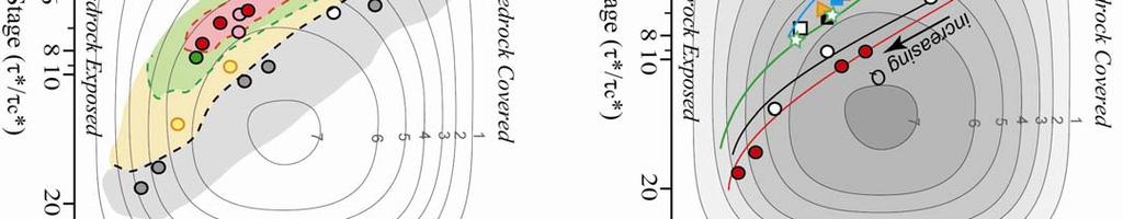
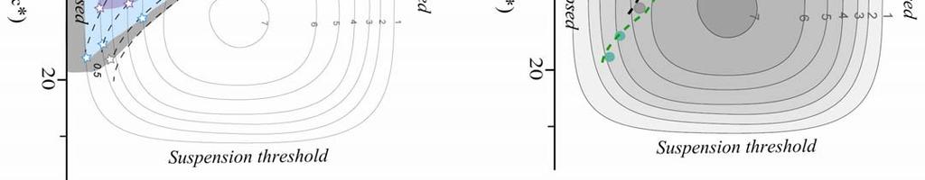
141 Chapter 5 Whittaker, 2007 Figure

142 Chapter 5 Whittaker, Do these data support the Sklar and Dietrich model? Although the experimental data confirm the basic message of the Sklar and Dietrich model, i.e. that erosion rates are heavily dependent on sediment flux and transport stage, the contour plot presented in Fig 5.8b clearly does not appear to resemble the predictions of the Sklar and Dietrich model in detail. In particular we document relatively small erosion rates for q s /q t =0.5, τ * /τ * c >8 where (dimensionless) rates of erosion are predicted to be the largest in the model, and we also document low-tomoderate rates of erosion for q s /q t ~1, again where erosion rates are predicted to be suppressed. Part of this is to do with our calculation of relative sediment supply and part of this is to do with the actual tank set-up. In particular, the contours of nondimensional erosion rates shown in Figure 5.8 assume a constant value of τ * c, but in our experiments, the changing pebble mass affects the packing density and hence the value of the critical shields stress. Consequently, the non-dimensional abrasion rate, E * 2 σ T ρ s 3 ( ) 2 = E / Y gd (eq. 28 in Sklar and Dietrich [2004]) would have to be * 2 * rewritten ( ) 2 E T / ρ sy gdτ c 3 = Eσ to keep a functional relationship between E* and E. This means that the 'elongate' shape of the contours of erosion is to be expected, as experiments with 10-25kg of sediment have critical shear stresses considerably lower than those with M >50kg, where the base of the flume is much nearer to being close packed. To effectively compare model predictions with our actual erosion data, we therefore need to convert model contours of E* to 'predicted' erosion contours, E predicted taking into account the changing critical Shields stress for experimental runs with differing sediment loadings. To do this, we calculate what happens to contours of E predicted when the critical shear stress is progressively lowered from the zone of approximately close packed values (i.e. constant τ * c, which means that E* is proportional to E) (Fig. 5.8d). Note that we are not trying to calculate absolute values of E predicted, merely seeing how the contours would be geometrically perturbed. Lines a-d on Fig 5.8d represent experimental trajectories for differing sediment mass in the tank (Fig 5.8a), and hence differing τ * c. Since E predicted ~ E*(τ * c ) 1.5, a reduction of τ * c by ~30% (for M =40kg relative to M=70kg) results in a reduction in E predicted by a factor of 2 relative to E*. Using this methodology, we can therefore contour the graph using the intersection of the lines a-d with the modeled contours of E* (marked with stars), to calculate new values of E predicted. 133

143 Chapter 5 Whittaker, 2007 To the left of line a, E predicted contours follow E* because we assume there is no variation in critical shields stress in this region. However, values of E predicted wrap sharply around a relative maximum of ~5 (at q s /q t =0.4; τ * /τ * c ~ 6), and as the critical shield stress declines from close-packed values, and all contours lie to the right of line d (where the critical shields stress is only 17% of the close-packed value), and hence the predicted erosion rates are only 7% of E*. To first order, these predicted contours mirror much more successfully the measured values of E in Figure 5.8c, with an 8- fold variation in erosion rates measured, and ~10 fold variation predicted from the geometrical analysis above. In particular the shape of the measured erosion contours (Fig. 5.8c) is largely a good match for the E predicted contours (Fig 5.8d), although any uncertainty in the estimate of the critical shield stresses at low packing density will necessarily affect the precise shape and pattern of the predicted contour surface. However, there remain some differences between the model predictions and our values, particularly the high recorded erosion values where q s /q t >0.7, and τ * /τ * c <5. In part this is due to over-prediction of pebble velocities at low stage (and hence overestimating sediment flux), but we would need to have over-estimated V p by ~40% for this to be sole explanation. Moreover, the way in which Sklar and Dietrich parameterise the fraction of bed-exposed, (F =1-q s /q t ) to estimate E* is not ideally suited to our tank set-up. Although perhaps meaningful in a statistical sense for a natural river (in terms of either a spatial or temporal balance of supply to transport acting to control exposure), it is not necessarily appropriate for describing exposure in a closed system like a circular flume, where the added sediments are not close packed. This is because as soon as a pebble is set in motion it is almost certain to strike the bedrock at some point, even if the sediment flux is close to the transport capacity, producing significant rate of abrasion for high q s /q t. We therefore would anticipate moderate erosion rates even when the relative sediment flux is high. 5.5 Influence of grain-size and lithology on sediment-flux dependent abrasion Grain-size A crucial question in understanding the abrasive capacity of fluvial flows is the extent to which the grain-size of entrained sediment determines the abrasive capacity of the river. Arguably, larger pebbles impact the channel bed with more energy than sediment with a smaller calibre, but for a set sediment flux, there are many more 134

144 Chapter 5 Whittaker, 2007 impacts per unit time if the grain size is lower, as there will, by necessity, be more pebbles in circulation. To address these competing effects we also assessed the erosive capacity of smaller limestone pebbles, 1-2 cm in size, on the same Miocene sandstone bedrock. Runs were completed using between 20 and 70 kg worth of pebbles at pump discharges between 260 and 400 m 3 hr -1 (Table 5.1); this is an identical range of pump discharges as used for the larger pebbles and corresponds to fluid flow speed in the flume of m/s. Figure 5.9 shows measured erosion rates as (a) function of pump discharge/fluid velocity and (b) and mass of pebbles in the tank, in an identical manner to Figure 5.4. Surprisingly, for increasing discharges (or water speeds) erosion rates vary only by a factor of 2, almost independently of the amount of added sediment. In addition, they display a decrease in the abrasion rate at higher pump discharges (i.e. water velocities > 3 m/s) which is suggestive of decreasing rate of pebble impact as the length of individual saltation hops increases with higher flow speeds. Importantly, compared to the larger 6-8 cm pebbles results this maximum occurs at lower pump discharge, which is compatible with the fact that small pebbles move and jump more easily than larger grains for any given shear stress. When the same measurements are presented in terms of mass loss against pebble mass in tank as a proxy for sediment flux (Fig. 5.9b), the data demonstrate that erosion rates are either constant with increasing amount of sediment, or even decrease in the case of pump discharges of ~350 m 3 /hr (velocity of 3 m/s). Given that mass loss from the plates will be negligible with no sediment in the tank, this suggests that maximum abrasion values must lie in the range of 0<M<25 kg, for the fluid velocities documented here (and we note that as the base of the tank is close-packed for M =18 kg all the quantity of sediment used here is enough to cover the base of the tank times (see Table 5.2)). Consequently, our raw data are best interpreted as supporting the coverage effect, and by inference, a tools effect for small mass loadings (dashed lines). 135

145 Chapter 5 Whittaker, 2007 Figure 5.9 Mass loss, E (g/hr), and vertical erosion rate, ε (mm/hr), for sandstone plates abraded by 1-2 cm pebbles as a function of (a) Pump discharge, Q (m 3 /hr) and (b) pebble mass, M (kg). The grey bar represents the point at which the base of the tank becomes close packed, and the dashed lines infer erosion rates for low sediment loads, assuming that mass loss is negligible for M = 0. To test these inferences, we analyze the abrasion results using 1-2 cm pebbles in (τ * /τ * c q s /q t ) space as before. Unlike the experiments with 6-8 cm pebbles, the floor of the flume is close packed, so here we can legitimately assume a constant critical threshold of entrainment and represent our data according to Sklar and Dietrich's nondimensional framework. According to our observations (Fig. 5.7) that partial motion is effective for τ * < 0.07 in experiments with 17 kg and 34 kg of 1-2 cm gravels, we hypothesize that τ * c 0.06, as derived from Shields experimental curve [1936]. Figure 5.10a shows measured erosion rates as a function of excess shear stress and relative sediment supply for sediment of this smaller calibre, while Figure 5.10b directly compares the erosion rates obtained in this study with the predictions of Sklar 136

146 Chapter 5 Whittaker, 2007 and Dietrich's [2004] model. Note that because the sediment calibre and critical shields stress for entrainment are constant in all the experiments with 1-2cm pebbles, measured mass loss, E should be proportional to the contours of non-dimensional erosion rate, E*. To first order, our results, which follow an arcuate trajectory in τ * /τ * c q s /q t space, (Fig. 5.10a) fit their general conclusions: erosion rates increase markedly as the transport stage rises, and concomitantly, as the sediment flux falls with respect to the transport capacity ( i.e. from q s /q t = 1 to q s /q t <<1). This verifies the importance of the coverage effect. Abrasion rates are at a maximum at intermediate values (q s /q t ~0.5) before falling off when the sediment supply is low and the transport stage high. Despite sparse data, a maximum abrasion rate seems to be obtained for transport stage of 12-15, in fair agreement with Sklar and Dietrich's model (Fig 5.10b). However, our data do highlight some sharp deviations from their theoretical predictions. At the highest transport stage obtained (τ * /τ * c ~25), the abrasion rate still represents 60% of the maximum value where theoretical predictions of the saltation/suspension transition at such excess shear stresses would suggest abrasion rates should be ~4 times lower, due to relatively infrequent impacts (τ * /τ * c for suspension is ~38 for 1-2 cm pebbles [Sklar and Dietrich, 2004; their fig. 8]). Overall the abrasion 'hump' appears to be shallower than the model predicts: for τ * /τ * c ~5-6, there is only a 1.5x variation in measured erosion rates as the relative sediment supply falls from 1 to 0.7, compared with a >5x variation predicted by the model. In part, this is due to the fact that we record non-zero erosion rates even when sediment flux balances the transport capacity. It is important to contrast the relative magnitude of erosion rates achieved with the 1-2cm pebbles with the rates obtained using the larger 6-8 cm size class. None of the experiments with the smaller-calibre gravel managed to replicate the erosion rates achieved with the larger pebbles, with maximum values (for M=50 kg; 350 m 3 /hr) being ~45% of those obtained with the 6-8 cm size class. In theory (eq. 28, Sklar and Dietrich, [2004]), we would expect peak erosion rates to vary as function of grainsize, specifically, being proportional to D 3/2. In our case this would imply a factor of 10 between experiments using these two different grain-sizes. Such difference between our data and theory is difficult to resolve: although we have not necessarily reached the maximum possible erosion rates with the 6-8 cm pebbles, (because the flume is not close-packed at high transport stage (Fig. 5.7)) we have probably reached >70% of this total (comparing E predicted and E* contours, Fig. 5.8d). Moreover, we 137

147 Chapter 5 Whittaker, 2007 appear to be near to the maximum erosion rates for the 1-2 cm pebbles (Fig. 5.9b; Fig, 5.10). This gives a likely factor of 3 in terms of difference in maximum abrasion rates between the runs with different grain-sizes, and it is difficult to envisage that a factor of 10 has been lost in the data. Consequently, these observations actually suggest that the magnitude of the sediment flux peak may be relatively inhibited at larger grainsizes, or put another way, that the erosion rate would have to scale as D 0.5 to fit a power-law relationship for the sediment sizes investigated here. In any case, we cannot collapse the data onto one single surface for E* as the Sklar and Dietrich model suggests. Figure 5.10 (a) 3-D depiction of erosion rate, ε (mm/hr) and mass loss, E (g/hr) against relative sediment flux (q s /q t ) and transport stage (τ * /τ * c ) for 1-2cm pebbles. Brown ovals show projection of the data on to the q s /q t - τ * /τ * c plain, and the data are colour coded by erosion rate category (see Fig. 5.10b). (b) Contour diagram of the data in Fig. 5.10a in comparison with Sklar and Dietrich's [2004] predictions of E* (grey lines). For constant τ * c and D, E ~ E*. To first order the data fit this pattern. 138

148 Chapter 5 Whittaker, Lithology In addition to grain-size, lithology is also recognised as a pre-eminent control on bedrock abrasion rates [Lavé and Avouac, 2001; Sklar & Dietrich, 2001]. We therefore compared results obtained from the slabs of Miocene sandstone with those generated using limestone bedrock (in this case a Tithonian limestone of identical lithology to the eroding pebbles) to assess the extent to which rock type controlled both the magnitude of the abrasion process, and also the distribution of mass loss as a function of relative sediment supply and excess shear stress. The tensile strength of this rock is 7.5 MPa compared to 2 MPa for the sandstone (section 5.3). Figure 5.11a shows the abrasion rates for different sediment masses added to the flume, using limestone pebbles of diameters of 6-8 cm (white squares) and 4-6 cm (black squares), compared with corresponding rates of erosion generated using sandstone bedrock (red envelope: see also Fig. 5.4) for an identical pump discharge of Q=350 m 3 /h in each case. Following the analysis presented in section 5.4, Figure 5.11b shows these data first as a trajectory in q s /q t τ * /τ * c space with increasing mass, while Figure 5.11c presents the results in E τ * /τ * c space; the x-axis is the same in both cases. A number of important findings can be drawn from these results: 1) Maximum abrasion rates with limestone (~5 g/hr or 0.2 mm/hr lowering rate) are obtained for M=50 kg, q s /q t = 0.4, τ * * /τ c ~5, and are approximately times less than those obtained using sandstone (90 g/hr), demonstrating the strong control of lithology on rates of abrasion - i.e. >16 fold decrease in abrasion rates for a <4 fold increase in tensile strength. 2) The limestone bedrock shows an almost identical pattern of erosion dynamics to that of the Miocene sandstone, particularly for the 6-8cm pebble class. For the same arcuate trajectory in q s /q t τ * /τ * c space, (Fig. 5.11b) generated by increasing pebblemass whilst holding pump discharge constant, both show a peak in erosion rate for identical experimental set-ups (M=50 kg; Q =350 m 3 /hr) (Fig. 5.11a) and very similar values of relative sediment flux and transport stage (Fig. 5.11b,c). The other limestone data points mirror the distribution of erosion rates for sandstone, but are consistently around 1/15-1/20th of the value of the latter, suggesting that whilst the rate of abrasion is highly sensitive to hardness of the bedrock, the actual dynamics of the abrasion process is not [c.f. Sklar and Dietrich, 2001]. As the abrasion process is largely one of brittle deformation wear, these results also mean that the effects of other process such as scratching (theoretically important at low angles of pebble 139

149 Chapter 5 Whittaker, 2007 impact) or ductile deformation are dominated by the abrasion-driven mass loss, whatever the nature of the substrate (in this case finely crystallized microstructure versus a poorly cemented granular material). This raises the possibility that abrasion rate data from one substrate could be converted easily into predictions for another given appropriate mechanical proprieties (e.g. rock mass strength data, Young's Modulus etc). Figure 5.11 (a) Mass loss, E (g/hr) (left hand y-axis) against mass of pebbles in the tank, for limestone plates abraded by 6-8 and 4-6 cm pebbles at a constant pump discharge of 350 m 3 /hr. Red swath depicts mass loss range for sandstone bedrock (right hand y-axis) abraded by 6-8 cm pebbles under identical conditions (see Fig. 5.4). (b) Relative sediment flux (q s /q t ) against transport stage, τ * /τ c *, for the three data sets presented in (a). Arrow shows trajectory of the results in (q s /q t τ * /τ c * ) space for experiments with increasing pebble mass but constant discharge. (c) Mass loss, E (g/hr) for limestone bedrock (left) and sandstone bedrock (right) for changing transport stage. Note the similar pattern of results for limestone and sandstone bedrock abraded by 6-8 cm pebbles despite a >16 fold difference in absolute abrasion rates. 140

150 Chapter 5 Whittaker, ) Results for the 4-6 and 6-8 cm pebbles are very similar (typically within 10% of each other, and at maximum by <22%). These results again suggest that the grain size does not represent a major control on abrasion rate, as previously suggested from the comparison between 1-2 cm and 6-8 cm calibre pebbles, where documented maximum erosion rates varied only by a factor of Discussion Importance of sediment flux The experimental flume tank results, presented above, confirm theoretical predictions of the importance of entrained sediment in determining the erosive capacity of rivers in bedrock settings. Small changes (<20%) in either relative sediment supply, q s /q t, or excess shear stress, τ * /τ * c, can generate significant changes (>600%) in the measured rates of bedrock abrasion. The results are, to first order, consistent with the general predictions of the Sklar and Dietrich [2004] model, and document an important role for the 'tools' effect, indicating that 'under-capacity' models of fluvial erosion [e.g. Beaumont et al, 1992], where sediment can only act to diminish erosion rates are inappropriate in bedrock settings. These findings apply for different lithologies, and differing grain-sizes, although we document a weaker control of sediment calibre on bedrock abrasion rates than Sklar and Dietrich suggest, implying that the rate of mass loss cannot be represented on a single non-dimensional surface in q s /q t τ * /τ * c space. Bedrock erosion laws which do not take into account sediment supply are therefore unsuitable for quantifying river incision rates if it cannot be demonstrated that the fluvial system lies at or close to the detachment-limited end-member, and the results suggest that sediment-flux dependent incision should be more readily incorporated within landscape evolution models [c.f. Gasparini et al., 2006]. However, it is important to be clear about the precise scope of these findings: below we discuss the limitations of this study and also the broader implications our results have in the field of fluvial geomorphology Study Limitations There are obviously some very evident limitations to the type of experimental methodology employed here. Firstly, relative sediment supply in real rivers is a dynamic variable in both space and time, and over a range of scales. In particular it 141

151 Chapter 5 Whittaker, 2007 will vary from flood to flood, and will evolve downstream, as tributaries supply sediment with differing median grain-size, and as in-situ bedrock erosion provides additional sediment to the flowing water. In contrast, in our experiments, we externally fix, in advance, both the sediment supply and the excess shear stress by choosing the quantity of material added to the flume tank, and the pump discharge used. However, this approach does have the decisive advantage of allowing us to vary pebble flux in carefully controlled increments, and hence probe in detail the way in which bedrock abrasion rates respond small changes in sediment flux or fluid speed. This precision is required to enable us to contour the abrasion surface in q s /q t τ * /τ * c space and to test the specific predictions of the Sklar and Dietrich model. Additionally, our experiments are carried out for a restricted range of grainsizes, whereas 'real' rivers obviously carry a varied array of material as saltating bedload, controlled both by the magnitude of the entraining flow and the size and availability of sediment in the channel [e.g. Paola and Seal, 1995; Rice, 1998, Mueller and Pitlick, 2005]. Such effects make predictions of erosion rate non-trivial, and we do not seek to reproduce this complexity in the lab; instead we contend that using a limited range of grain-sizes in each run allows us to explore some of the first order effects of sediment caliber on bedrock abrasion rate, while simultaneously avoiding the problem of a non-uniform radial distribution of pebble size during flume operation. It is clear that mixed grain-size flows would tend to display a more diffuse erosion rate maximum as a function of excess shear stress, because smaller pebbles could be mobile at low fluid velocities, whilst larger sizes would still be immobile, but the fact that smaller grain-size fractions are not equally erosive for a given sediment supply (Fig. 5.9) means that a non-linear response would still be maintained. We have largely concentrated on abrasion of bedrock by mono-lithological limestone pebbles which are either harder than their substrate (in the case of sandstone bedrock) or identical to it (for carbonate bedrock). As outlined in section 5.3, this contrast reflects the real-life bed-load situation found in areas around the world, and specifically in the Central Apennines of Italy [Whittaker et al., 2007a]. Moreover we contend that, in general, cases where bedrock is eroded by pebbles that are either a similar lithology or are harder than the substrate, are probably the most geologically common scenario: Any sediment supplied to a channel that is considerably more erodable than the bedrock it has to move over would tend to be diminished in size very rapidly, and would have only a limited influence on long-term abrasion rates [c.f. Attal and Lavé, 2006]. We do not doubt that a different selection of pebble lithology 142

152 Chapter 5 Whittaker, 2007 could generate different numerical values of erosion rate, but we believe that the relative distribution of abrasion rates would remain similar. Finally, it is important to note that the results presented in this paper concern only mass loss from bedrock by saltating bedload abrasion; we do not consider other potentially important processes of wear such as plucking, fracturing or cavitation [Whipple et al., 2000a]. Indeed we have deliberately excluded data for bedrock blocks where large pieces of material have been visually detached during a single experimental run (section 5.4). Consequently, although we show in Fig that the magnitude of mass loss through bedrock abrasion is dependent on lithology, but the pattern with increasing transport stage or sediment flux is not, this is definitively not the same as saying that abrasion is the only process that matters when assessing longterm erosion rates. Specifically, while visual inspection of the (relatively friable) sandstone blocks before and after each experiment indicates wear almost solely by abrasion processes, we do observe that plucking and subsequent excavation of microfractures does periodically occur for limestone bedrock samples. For 15 runs involving limestone (hence 45 individual blocks) demonstrable loss of material through non-abrasive processes (Fig. 5.12a) occurred on two occasions i.e. 5% of the time. In these cases, the mass loss was 5-9 times the average of the other two blocks, despite their being no sign of significant fractures at the time the bedrock was mounted. In comparison incipient fractures appeared in the sandstone (Fig. 5.12b) on only 2 occasions out of 150 sample-runs (1.3% of occasions) with attendant erosion rates being only 2x higher than the 'average' rate. We ascribe this to the fact that while the 'background' rate of erosion is times higher in the sandstone bedrock compared to the limestone bedrock, the typical size of rock chips lost through plucking and fracturing scales by a much smaller factor between the two lithologies. This means that for homogenous, granular media, such as sandstone, abrasion rates from lab experiments are probably comparable to erosion rates of bedrock in toto, whilst in heterogeneous, fractured lithologies, average rates of bedrock erosion (defined as the cumulative sum of all attrition processes) could be considerably higher than the abrasion data taken alone would suggest. Nevertheless, visual inspection of fractured bedrock slabs at the end of experimental runs points to the importance of smaller pebbles wedging into the growing crack, which then act as a 'chisel' to remove whole pieces of rock. This wedging effect must also be a function of sediment flux, and would presumably be suppressed for sediment-starved catchments. 143

153 Chapter 5 Whittaker, 2007 Figure 5.12 (a) Limestone bedrock slice where a micro-fracture has been excavated by pebble wedging, forming a large crack. In this case, the documented mass loss was more than 5 times the other bedrock slices under the same experimental conditions. (b) Sandstone bedrock slice where a micro-fracture has been excavated by pebble wedging. In this case the mass loss was only 1.5x greater than the other bedrock slices under the same experimental conditions Wider Geomorphic Implications Having acknowledging the caveats above, these laboratory results do have significant implications for understanding and predicting the longer-term geomorphic evolution of fluvially-mediated landscapes. Although recent work has shown that fluvial erosivity can be enhanced by decoupling channel geometry from drainage area and slope [chapter 2; Whittaker et al., 2007a] and that this can have a significant impact on the style and tempo of landscape evolution [chapter 3; Whittaker et al., 2007b], these experimental data strongly imply that long term variations in sediment supply to catchments could also exert a similar control on geomorphic development. Firstly, the fact that bedrock abrasion rates are a non-linear function of sediment supply allows for small changes in river discharge, for example caused by 144

154 Chapter 5 Whittaker, 2007 changing precipitation rates over glacial/interglacial cycles, to lead to quite considerable changes in long term rates of landscape down-cutting [c.f. Tucker and Slingerland, 1997]. This effect would be most noticeable if the trajectory of typical flood events in q s /q t τ * * /τ c space were to be shifted significantly relative to the theoretical erosion maximum. The first-order implication of this is that fluvial landscapes could be more sensitive to the effects future climate change (such as changing rates and annual distribution of rainfall) than might be expected from conventional (i.e. discharge driven) stream power models, even if one included an erosion threshold [c.f. Snyder et al., 2003b]. Secondly, the data require us to re-examine carefully our notion that high discharge events are always likely to be the most erosive flows. In fact, as bedrock abrasion rate is controlled by relative sediment supply as a function of transport stage, then it follows that smaller magnitude flows are likely to be geomorphically the most significant assuming that the available sediment to be moved through the catchment is either finite and/or weighted towards smaller-grain sizes: i.e. the largest flows are likely to have a lower ratio of sediment supply to transport capacity, and higher excess shear stress, limiting their erosive power, whilst flows of intermediate discharge are more likely to hit the abrasion maximum. Such effects are likely to be magnified in catchments where the bedrock is relatively weak and granular, and hence abrasion is the dominant process of wear. The above points can be put into context by considering that the rates of down-cutting documented in these experiments (typically of the order of ~1 mm/hour for sandstone and ~ mm/hour for limestone) are readily comparable to yearly rates of denudation evidenced from mountainous areas such as the Western Alps (~1mm/yr) [Brocard et al., 2003], Taiwan (~10 mm/yr) [Hartshorn et al., 2002; Dadson et al., 2003], and the Central Apennines (0.2-2 mm/yr) [Roberts and Michetti, 2004; Whittaker et al., 2007b], where the experimental set-up presented in this paper replicates typical bedrock/sediment conditions found in upland rivers in the region. In the latter case, the fact that estimates of long-term annual bedrock erosion rates are the same order of magnitude as experimental abrasion results over just one hour at flood stage, explicitly points to the delicate interaction of flood frequency and sediment coverage of the bed in governing the erosional dynamics of mountain belts (i.e. in the Apennine case, the most erosive combinations of relative sediment supply and transport stage must rarely occur at present), and emphasizes the potential sensitivity of fluvial incision rates to changes in boundary conditions. These observations 145

155 Chapter 5 Whittaker, 2007 highlight the fact that quantifying the effect of differing sediment fluxes on landscape evolution remains an outstanding objective in the field of geomorphology, particularly with respect to the timescale over which changes in q s become recorded in the landscape. 5.7 Conclusions The experimental results presented here constitute a unique data set that explicitly quantifies the effect of relative sediment flux, q s /q t, and excess shear stress, τ * * /τ c, on bedrock abrasion rates under fluvial conditions. We demonstrate that rates of abrasion wear by saltating bedload are a strongly non-linear function of both sediment supply and transport stage, and that small changes (<20%) in either parameter can lead to >5 fold variation in measured erosion rates. In particular, our data actively support the hypothesis that sediment has a dual effect on bedrock abrasion rates: at low relative sediment supply, small increases in sediment flux promote higher erosion rates because there are more tools acting on the bed, whereas at high sediment supply further increases in sediment diminish erosion rates as the substrate becomes progressively more covered. These results verify the original tools/coverage hypothesis of Gilbert [1877] and clearly show that fluvial erosion models that allow sediment to enhance as well as diminish abrasion rates [e.g Sklar and Dietrich, 2001; Sklar and Dietrich, 2004] are much better descriptors of physical reality than those which only allow sediment to reduce the rate of bedrock erosion [e.g. Beaumont et al., 1992; Koii and Beaumont, 1994]. We also demonstrate that transport stage has a similar dual effect on bedrock abrasion rates: with increasing excess shear stress, bedrock abrasion rates increase as pebble velocity is higher, and the particles therefore impact the bed with greater energy. However, at higher transport stages, erosion rates fall, because the high pebble speed results in longer saltation hops and hence fewer impacts. To first order, our findings are in fair agreement with the predictions of the Sklar and Dietrich's [2004] model; for example, we obtain maximum erosion rates at q s /q t ~ , i.e. when the sediment supply is half the theoretical transport capacity for experiments regardless of grain-size, and we find that for experimental set-ups where a constant critical shields stress for entrainment can be assumed, erosion rates peak at transport stages of ~14, as Sklar and Dietrich predict. However, we do document significant deviations from their model predictions; most notably that 146

156 Chapter 5 Whittaker, 2007 erosion rates appear to scale with grain-size to a considerably lower power than they predict (i.e. D 0.5 rather than D 1.5 ) and that we can generate measureable rates of bedrock abrasion even when the sediment flux is approaching the theoretical transport capacity of the flow. We find that these results hold for both sandstone and limestone bedrock with tensile strengths of 2MPa and 7.5MPa, respectively, although the former erodes at rates up to 20 times greater than the latter. These results suggest that while the magnitude of the abrasion rate may be controlled by lithology, the pattern of erosion as a function of transport stage and relative sediment flux is not. This raises the possibility that rock bulk properties could be used to scale-up abrasion rates between differing lithologies. Finally, the vertical rates of erosion documented here (>1mm/hour for sandstone) are comparable in magnitude to yearly estimates of downcutting in many mountain belts, and emphasize that the interplay between sediment flux, flood magnitude and bed coverage is vital for understanding the long term effect of sediment flux in fluvially mediated landscapes. 5.8 Notation ε vertical erosion rate [L T -1 ]. ρ f density of fluid in flume [M L -3 ] ρ s density of sediment in flume [M L -3 ] Δρ buoyant density of sediment in flume, [M L -3 ] τ b shear stress on base of tank [ML -1 T -2 ] τ i shear stress on inner wall of tank [ML -1 T -2 ] τ o shear stress on outer wall of tank [ML -1 T -2 ] τ * * τ c D Shields stress, dimensionless. critical Shields Stress, dimensionless gravel mean diameter [L]. E mass loss rate of the rock plates [M T -1 ] E* non-dimensional erosion rate [c.f. Sklar and Dietrich, 2004] f Darcy-Weisbach friction factor, dimensionless F Fraction of bedrock exposed, dimensionless g acceleration due to gravity [L T -2 ] h i h w height of inner wall of flume [L] height of water over-flow above inner wall of flume [L] I particle impact rate per unit area [L -2 ] 147

157 Chapter 5 Whittaker, 2007 M mass of sediment added to the flume [M]. p packing density of pebbles on the bed of the flume (ratio of total projected sediment area to bed area), dimensionless q s sediment flux per width unit in the flume[m L -1 T -1 ]. q t sediment transport capacity in the flume [M L -1 T -1 ]. Q pump discharge for flume [L 3 T -1 ] r m r i r o T p mean radius of flume tank [L] inner radius of flume tank [L] outer radius of flume tank [L] average time taken for a pebble to make one circuit of the flume [T] U i injection velocity of water into flume [L T -1 ] V average volume of rock detached on impact [L 3 ] V p average pebble velocity in flume [L T -1 ] V w average fluid velcoity in flume [L T -1 ] W width of flume tank [L] ΔZ height of vortex created during flume operation [L] PAPER ACKNOWLEDGEMENTS A. Whittaker was supported from an Entente Cordiale (UK-France) Scholarship and the Natural Environment Research Council (UK), and J. Lavé & M. Attal were supported by the Institut National Des Sciences de L'Univers programmes coup de pouce and programme national de recherches en hydrologie (France). Experimental work was conducted at the Laboratoire de Géodynamique de Chaînes Alpines, UJF Grenoble; Jean Paul Maçon (Laboratoire de Géophysique Interne et Tectonophysique) provided considerable technical assistance. AUTHOR CONTRIBUTIONS As first author, I confirm that I wrote the text, prepared all the diagrams and developed the intellectual arguments presented herein. J. Lavé (thesis supervisor) helped to define the scope of this research, and clarified the mathematical basis for the relative sediment supply/excess shear stress analysis in section He also supplied some of the data presented in Fig M Attal designed the flume and gave technical advice on how to adapt the base to incorporate bedrock slabs. He also provided the data presented in Fig

158 Table 5.1 Sandstone results 6-8cm: Q run n# M duration ΔZ V w τ b τ * τ */ τ c * V p q s q t q s /q t E raw correction E error a b

159 cm: Q run n# M duration ΔZ V w τ b τ * τ */ τ c * V p q s q t q s /q t E raw correction E error

160 Limestone Results 4-6cm: Q run n# M duration ΔZ V w τ b τ * τ */ τ c * V p q s q t q s /q t E raw correction E error cm: Q run n# M duration ΔZ V w τ b τ * τ */ τ c * V p q s q t q s /q t E raw correction E error Symbols: Q pump discharge (m3/hr) τ b basal shear stress, (Pa) q s sediment flux (kg/m/s) M sediment mass (kg) τ * Shields stress (dimensionless) q t transport capacity (kg/m/s) ΔZ height of flume vortex (cm) τ */ τ c * Excess shear stress (i.e. transport stage) E raw mass loss from bedrock (g/hr) V w Water velocity (m/s) V p pebble velocity (m/s) correction pebble density correction factor (Fig. 5.5.) E corrected bedrock mass loss (g/hr) error + erosion rate disparity between plates (g/hr)

161 Table 5 2 Sediment mass, M (kg) pebble volume (m 3 ) pebble no. area of pebbles (m 2 ) packing density 6-8 cm pebbles cm pebbles cm pebbles Area of flume floor = 1.13m 3

162 Chapter 6 Whittaker DISCUSSION AND SYNTHESIS 6.1 Overview and Synthesis This thesis has used an integrated approach of field, DEM and lab-based studies to investigate the key controls on the behaviour and incisional capability of upland 'bedrock' channels. These rivers play a fundamental role in determining the timeintegrated relief structure of the earth's surface, and are largely responsible for transmitting climatic and tectonic signals to the landscape (section 1.2). The need for a greater understanding of the dynamics of the river system has been increasingly recognised as an outstanding challenge within the field of the geosciences over the last ten years (section ) [c.f. Tinkler and Wohl, 1998] and the work presented within this thesis makes a decisive contribution towards meeting this aim. Specifically, the papers presented in this thesis, although forming stand-alone contributions to the research literature in their own right, constitute a coherent strategy for probing different aspects of bedrock river dynamics. Firstly, chapters 2-4 used the Central Apennines of Italy as a natural laboratory to study the way in which rivers behave when perturbed by tectonic forcing. The approach here is to look first at an individual channel crossing an active normal fault where we have excellent constraints on the timing and magnitude of the tectonic forcing, and then to progressively widen the study to compare the results with two other rivers crossing faults with different, but equally well constrained spatial and temporal distributions of uplift (chapter 3). The insights gained from the previous two chapters were then applied to a wider study of rivers crossing active faults throughout the Central Apennines (chapter 4). These results have been complemented with lab-based work on the mechanics of bedrock erosion, specifically the experimental calibration of bedrock abrasion rates as a function of sediment flux and transport stage, using similar rock types to those found in the field study areas (chapter 5). Important research contributions of this thesis include: demonstrating that a key way in which rivers adjust to an increase in fault uplift-rate is by decoupling channel geometry, particularly high-flow channel width, from discharge/drainage area in the region of the fault, and that this makes a significant difference to the erosivity of the channel in the zone of maximum uplift (chapter 2). 153

163 Chapter 6 Whittaker 2007 defining diagnostic field criteria for identifying rivers near the detachmentlimited end member that are undergoing a transient response to tectonics, showing how such channels evolve towards topographic steady-state and calculating the response time for this to occur. I also demonstrate that some landscape features, such as narrow valley widths can be maintained even for steady-state channels crossing active faults, even if good hydraulic scaling has been re-established (chapter 3). showing how the vertical elevation of long profile convexities in transient channels appears to scale with the magnitude of uplift rate increase both between different faults in the Apennines, and also along strike for the same fault segment. These results establish that transient landscapes can act as an important archive of tectonic forcing over million year time-scales (chapter 4). quantifying explicitly the role of sediment in modulating bedrock abrasion rates, and demonstrating that small changes (<20%) in relative sediment supply or excess shear stress can lead to significant changes in bedrock abrasion rates (by almost one order of magnitude in some circumstances). These are the first experimental results to demonstrate these effects using a flume that replicates real fluvial entrainment processes, and enable us to calibrate the Sklar and Dietrich [2004] model of sediment influenced abrasion (chapter 5). Below I discuss the importance of these key discoveries, and highlight the wider implications of the results within the context of landscape dynamics. Finally I detail some of the on-going and future work that is or has been directly motivated by the findings presented in this thesis. 6.2 Study Results: Importance, impact, implications Detecting transient responses, clarifying erosion laws The results presented in chapters 2-4 constitute the first set of field observations to have explicitly characterised transient bedrock river response to tectonic perturbation. In particular I have shown that all the rivers crossing active normal faults that have undergone an increase in uplift rate within the last 1My are characterised by significant long profile convexities, whilst those crossing constant-slip rate faults have 154

164 Chapter 6 Whittaker 2007 concave-up long profiles. Additionally field-observations show that the Italian catchments are generally starved of sediment, with shields stresses well above the transport-limited threshold [c.f. Mueller and Pitlick, 2005]. These results constitute an unambiguous validation of the modelling predictions of Tucker and Whipple [2002] - i.e. that in response to an increase in uplift rate, channels approaching the detachmentlimited end-member should develop a knickzone that propagates upstream through time [see Fig. 1.1]. However, our data on knickzone migration rates demonstrate that they propagate with greater velocity when the fault slip-rate is high. This is consistent with n>1 in the classic detachment-limited stream-power model, but could also be explained by a role for sediment in enhancing erosion rates: i.e. the rivers in the Italian Apennines are close to, but not quite at the detachment-limited end-member. The work is a significant step forward from previous studies that have attempted to calibrate erosion laws [e.g. Van der Beek and Bishop, 2003; Tomkin et al., 2003] because I have identified a setting where the transient response to an explicit perturbation can be clearly captured Hydraulic scaling A key finding of this thesis has been that traditional hydraulic scaling algorithms, which parameterise aspects of channel geometry, such as depth and width, as power law functions of discharge or drainage area (i.e. W ~ A 0.5 [Leopold and Maddock, 1953]) are inappropriate for rivers close to the detachment-limited end member which are undergoing a transient response to tectonics. In reality, transient channel narrowing in the vicinity of the fault helps the river to maximise its stream-power, and explains why rivers are not always defeated or deflected by continuing uplift. The results also emphasize that a sophisticated understanding of river-response to tectonic forcing is vital to accurately predict the locus and timing of sediment input to adjacent basins. The findings further imply that any field study that employs erosion 'laws' that depend on scaling relationships between width and drainage area may significantly under-estimate fluvial erosivity in tectonically active areas. This is true even if the exponent on a discharge-dependent power-law is derived from field data [c.f. Duvall et al., 2004], because log-log plots can be misleading in these settings (chapter 3). Secondly, it means that the current generation of landscape models, which tend to explicitly or implicitly embed steady-state hydraulic scaling within their erosion algorithms, need to be modified to take account of dynamic channel adjustment. This 155

165 Chapter 6 Whittaker 2007 is vital if we are going to successfully model landscape response to perturbation in external boundary conditions, because at present one of the key variables (i.e. channel width) is being incorrectly modelled. The findings from chapter 2 [c.f. Whittaker et al., 2007a] have already had a significant impact in this domain in terms of influencing key workers and promoting further work; the initial insights from this study [Whittaker et al., 2005] motivated Wobus et al., [2006b] to model explicitly how self-formed bedrock channels might dynamically adjust their geometry. It also provided the impetus for Cowie et al., [2006] to use a constant channel width in her study of the interactions between fault growth and drainage network evolution, and has recently led to Attal et al., [in review], to explicitly model the impact of dynamic channel adjustment on the dynamics and response time of transient landscapes Defining diagnostic criteria for transient landscapes An important aspect of this work has been to explicitly characterise fluvial (and wider landscape) response to tectonic forcing, and thus define diagnostic criteria for identifying transient landscapes in the field. In particular we show that for bedrock channels that are not in topographic steady-state, and are responding to an increase in tectonic uplift rate, they are characterised by: 1) poor hydraulic scaling, with channel widths decoupled from drainage area 2) channel aspect ratios that are a non-linear function of slope 3) narrow valley widths (i.e. gorge formation) 4) reduced variability in channel planform 5) unit-stream power distributions that are on a much shorter wave-length to faultuplift 6) coupled angle-of-repose hill-slopes 7) elevated coarse fraction grain-sizes of sediment, where it is present (related to landsliding bringing material of larger calibre into the channel). This is in addition to oft-cited presence of long-profile convexities. In contrast river systems that have reached topographic steady-state have good hydraulic scaling, and concave-up long profiles, but they may have narrow valley widths where they need to increase their incision rate towards an active fault (chapter 3). This is the first time that field criteria have been established for identifying transient river responses to tectonics, and as such has practical applications across the field of geomorphology, 156

166 Chapter 6 Whittaker 2007 from selecting the right method to extract tectonics from topography (below) to identifying areas where fluvial erosion models might be successfully evaluated Landscape response time and landscape sensitivity The data in chapters 3-4 have enabled me to estimate the response time of rivers in the Central Apennines to tectonic perturbation. Rivers crossing faults that underwent an increase in uplift rate at ~0.8 Ma are characterised by significant long-profile convexities, whereas rivers crossing faults which have had a constant slip-rate for 3My have concave-up longitudinal profiles, good hydraulic scaling and have reached topographic steady-state. However rivers crossing such faults do retain narrow valley widths over this time period. I also show that hill-slopes in the Rio Torto, near Fiamignano have responded at least as fast as the migration rate of the incisional wave generated since the increase in the fault uplift rate (in this case ~6 mm/yr). These results are significant because they demonstrate that the effects of tectonic perturbation (such as local channel steepening and loss of good hydraulic scaling) are retained in landscape, at least in this setting over relatively long periods >10 6 years (this is one order of magnitude larger than has been suggested for channels in the vicinity of the Mendocino Triple junction, California [Merrits and Vincent, 1989; Snyder et al., 2000]. The implication of this long response time is that the gross morphology of the landscape is likely to be rather insensitive to either short-term oscillations in boundary conditions (i.e. <10 4 years) or small amplitude variations (e.g. changes in relative uplift rate of <2). However, once the landscape starts to respond the effects are retained over long periods. My data also suggest that detachment-limited rivers crossing active normal faults are vulnerable to the beheading of the headwaters unless the migration rate of the knickzone is rapid, and this negative feedback acts to limit the time taken for the fluvial system to reach topographic steady-state to around 1My Tectonics from topography - the earth's surface as an archive of past events Another significant result that has emerged from this thesis is the fact that, for detachment-limited channels (or those close to this end-member) that are undergoing a transient response to tectonics, the vertical height of long-profile convexities, as measured from the fault, scales with the magnitude of the fault slip-rate increase 157

167 Chapter 6 Whittaker 2007 (chapter 4). Collaborative work using the CHILD landscape model [Tucker et al., 2001a] (run with slope dependent width scaling [Finnegan et al., 2005]) to reproduce a river incising across a back-tilting fault block, has allowed me to test these field observations. I demonstrate that the model compares well with the field data presented in this thesis, and additionally I show that the slope of a best fit line in {convex-reach height, uplift-rate increase}-space provides information on the time since the change in uplift rate occurred: i.e. the greater the gradient of the best-fit line, the longer the time since the tectonic perturbation. This result is important because it underlines the fact that transient landscapes can act as a 'tape-recorder' or archive of tectonic forcing and raises the prospect that this method could be applied to other tectonically active areas where uplift rates are presently poorly constrained. However, I also demonstrate that analysis of normalised steepness indices to deduce rock uplift rates is vulnerable to significant error if the channel is not in topographic steady state [c.f. Wobus et al., 2006a] Importance of sediment flux in determining fluvial erosivity A significant finding of chapter 5 is that sediment flux can play a vital role in determining the erosivity of river systems. Consequently, as noted in section 5.5, small changes in river discharge, or storminess over glacial to interglacial cycles, or due to future changes in rain-fall distribution could potentially lead to considerable changes in the short-term rates of fluvial erosion. Moreover, these findings also raise the prospect that small, but sustained differences in longer-term average sediment supply to catchments could play a definitive role in shaping their evolution and morphology. For example, catchments with ostensibly similar bedrock lithologies and sizes, and perturbed by a similar tectonic signal, but with differing relative sediment flux are likely to respond to this event in quite different ways. While I have shown that channels close to the detachment-limited end-member tend to react by significant local channel-steepening and narrowing, rivers with significant relative sediment flux are unlikely to respond in such an extreme manner: the available sediment in the latter case can do more of the incisional work, without such dramatic changes in channel geometry. In contrast, the steep convexities noted in the rivers in the Central Apennines are generated because the 'bedrock' channels in this area, which are largely starved of sediment and hence close to the detachment-limited endmember, are relatively ineffective in keeping pace with fault-uplift. As sediment in 158

168 Chapter 6 Whittaker 2007 the fluvial system comes to dominate, channel response should becomes more diffusive [Whipple and Tucker, 2002], and this also has significant implications for hill-slope coupling, the timing of sediment release to basins and the response time of the system [Cowie et al., 2006]. My experiments clearly show that to fully understand the long-term effects of sediment flux on landscape development, sediment supply-dependent incision needs to be incorporated more routinely into landscape models [c.f. Gasparini et al., 2006]. Moreover, the specifics of the conclusions drawn in chapters 2-4 strictly apply to channels close to the detachmentlimited end-member undergoing a transient response to tectonic uplift rate; this highlights the need for additional fieldwork to investigate the landscape sensitivity and evolution in fluvial environments where sediment is abundant (see section 6.3.3). 6.3 On-going and future work This work presented in this thesis has given rise to a range of ideas for future work. Below I give an outline of a project that is already under way, and list some other potential avenues for further research: Direct comparison of erosion rates, sediment flux and stream power in a transient setting. An obvious next step to take the results and ideas presented in this thesis forward is to directly compare our predictions of river erosivity (from width-adjusted unit streampower calculations - chapters 2-3) for channels in the Central Apennines with flumetank measurements of bedrock erodability. Lithologies used for the experiments presented in chapter 5 are very similar to those in the Central Apennines (indeed the sandstone was sourced from a quarry near the Rio Torto (chapter 2, Fig 2.1)). This means that the experimental bedrock erosion data are explicitly comparable with field sites in the Italian Apennines [c.f. Hartshorn et al., 2002]. In-situ measurements of downstream erosion rates for rivers undergoing a transient response to tectonics would: (a) give a unique insight into the extent to which predictions of the downstream of unit-stream power do match real bedrock erosion rates, and hence provide a test of how close Italian rivers are to the detachment-limited end-member and (b) enable the comparison of 'yearly' measurements of erosion rate in rivers crossing faults, with long-term fault uplift rates and lab-based calibrations of bedrock abrasion rates. This is particularly significant because lab-based measurements of 159

169 Chapter 6 Whittaker 2007 sandstone bedrock erosion rates during 1 hour of abrasion at high flow stage are comparable in terms of magnitude to yearly rates of fault uplift in the Apennines (i.e. 1mm/yr for fault uplift versus 1mm/hr for sandstone abrasion (section 5.5.3)), and thus emphasizes the clear importance of understanding the relationship between incision, discharge and sediment flux. An obvious place to start is the Rio Torto, crossing the Fiamignano fault (Fig. 2.1) whose hydraulic geometry, sediment calibre, and tectonic boundary conditions are already very well constrained [chapters 2-3; Whittaker et al., 2007a; Whittaker et al., 2007b]. In July 2005, I therefore set up a field experiment to monitor yearly to decadal erosion rates in the channel 1. The approach has been to drill up to 10 sets of 1 This work is in collaboration with Dr. Mikael Attal, School of GeoSciences, University of Edinburgh 2 Work in collaboration with Dr. Sarah Boulton, School of Earth, Ocean and Environmental Sciences, University of Plymouth. 3 This research is being led by Dr. Patience Cowie, School of GeoSciences, University of Edinburgh 160

170 Chapter 6 Whittaker 2007 holes, ~ 4 cm deep into the bedrock, at regular intervals downstream in the channel [Fig. 6.1], following an adapted version of the methodology of Hartshorn et al., [2002]. The depth of the holes was measured to within 0.2mm using callipers, and they were filled with hardwood dowel to a level flush with the bedrock. Erosion rates can be monitored by measuring how the depth of the drill-holes reduces through time. a Figure 6.1: (a) Bedrock drill site, at 7.5km downstream in the Rio Torto (b) (overleaf) Long profile of the Rio Torto, Showing location of drill sites (yellow). Blue line is raw elevation data from Italian DEM. Red line is best-fit moving average of elevation, verified with an altimetric GPS. Green dot shows position of photographs shown in Fig. 6.2 b fault drilling site site in Fig. 6.2 Although we do not plan to visit all the sites until next year (so that our results are time-averaged over 3 years), initial data from one monitoring site downstream of the active fault (i.e. in the hangingwall of the Fiamignano fault), highlighted in green in Fig 6.1a, and measured in October 2006 (an interval of 16 months), already 161

171 Chapter 6 Whittaker 2007 demonstrate bedrock erosion rates of several centimetres (Fig. 6.2). Such incision rates are obviously unsustainable catchment wide over time-periods >10 4 years, must indicate that the sediment coverage becomes a dominant control almost as soon as the river enters the hangingwall: i.e. the 16th month average is more than 25 times documented 'typical' Apennine long term incision rates of approximately 1 mm/yr [D'Agostino et al., 2001] yet could be achieved in just two high-flow floods if the abrasion maximum [Fig 5.8c] in relative sediment flux, transport stage space was maintained for a duration of four hours in each event. The inescapable conclusion is that the bed of the channel, on average, must spend its time covered by gravel, with erosion rates close to zero. These findings highlight the complex interactions between tectonic uplift rates, precipitation-driven river discharge, sediment flux and long-term erosion rates, and we hope this study will allow us to elucidate these controls in an environment where the tectonic boundary conditions and channel geometry are already well-constrained. 2.5cm height a b Figure 6.2: (a) Photograph of bedrock erosion after 16 months at site shown in green, Fig 6.2. Nine 4 cm dowels were emplaced flush into the bedrock; only two remained, giving erosion rates between 2.5 and 4 cm over 16 months. The site was exposed sandstone on the base of the channel when originally drilled in June 2005, but was buried by 20 cm of gravel by October 2006 (b) Close-up of dowel shown in Fig 6.2a 162