Douglas County/Carson City Travel Demand Model

Transcription

1 Douglas County/Carson City Travel Demand Model FINAL REPORT Nevada Department of Transportation Douglas County Prepared by Parsons May 2007

2 May 2007 CONTENTS 1. INTRODUCTION DEMOGRAPHIC INFORMATION... 4 Zone Structure... 4 Demographic Forecasting Needs... 4 Base Year (2005) Socioeconomic Data Summaries HIGHWAY NETWORK... 8 Network Development... 8 Transportation Analysis Zones and Highway Geographic Database... 8 Node Attributes Highway Network (.NET) Creation Turn Penalties Table Base Year Network Road Classification Highway Skims TRIP GENERATION Resident Model Set Overview Socioeconomic Submodels Base Year Data Households by Household Size Disaggregation Submodel Households by Income Group Disaggregation Model Estimating Joint Distributions of Households by Socioeconomic Strata Socioeconomic Model Application Summary Trip Production Models Home-Based Work Trip Production Model Home-Based School Trip Production Model Home-Based Shop Trip Production Model Home-Based Other Trip Production Model Non-Home-Based Trip Production Model Trip Attraction Models Home-Based Work Trip Attraction Model Home-Based School Trip Attraction Model Home-Based Shop Trip Attraction Model Home-Based Other Trip Attraction Model Non-Home-Based Trip Attraction Model Special Generator Trip Attraction Models TRIP DISTRIBUTION Introduction Gamma Function Source of Data iii

3 May 2007 Calibration Process Friction Factor Parameters Trip Length Frequency Distributions Trip Length Distribution Macro MODE SPLIT Introduction Home-Based Auto Occupancy Models Home-Based Work Average Auto Occupancies Home-Based School Average Auto Occupancies Home-Based Shop Average Auto Occupancies Home-Based Other Average Auto Occupancies Non-Home-Based Auto Occupancy Models TRIP ASSIGNMENT Production/Attraction to Origin/Destination and Time of Day Distribution Other Trips Matrix Traffic Assignment Cold Start Flows and VMT Feedback Looping Assignment Reports Traffic Assignment Validation TRAVEL FORECAST MODEL APPLICATION APPENDIX A: Input Files, Output Files, and Parameters APPENDIX B: 2005 Land OSC Data APPENDIX C: Douglas County and Carson City Industries and Travel Demand Model Employment Category iv

4 May 2007 LIST OF FIGURES Figure 1-1: Douglas County/Carson City Model Flow Chart... 2 Figure 2-1. Douglas County and Carson City Transportation Analysis Zone (TAZ) Map6 Figure 2-2. External Gateway Locations for the Travel Demand Model... 7 Figure 3-1: Year 2005 Douglas County and Carson City Highway Network Figure 4-1: Household Size Disaggregation Submodel Figure 4-2: Income Group Disaggregation Submodel Figure 5-1: Friction Factor Parameters Home-Based Work Figure 5-2: Friction Factor Parameters Other Trip Purposes Figure 5-3: Travel Time Frequency Distributions Home-Based Work Trips Figure 5-4: Trip Length Frequency Distributions Home-Based Work Trips Figure 5-5: Home-Based School Trips Frequency Distribution Figure 5-6: Home-Based Shop Trips Frequency Distribution Figure 5-7: Home-Based Other Trips Frequency Distribution Figure 5-8: Non-Home Based Trips Frequency Distribution Figure 6-1: Non-Home-Based Average Auto Occupancy Calibration Data and Model. 43 Figure 7-1: Screenline Locations in Carson City Figure 7-2: Screenline Locations in Douglas County Figure 7-3: Comparison of AM Peak Hour Volumes to Traffic Counts in Carson City. 53 Figure 7-4: Comparison of AM Peak Hour Volumes to Traffic Counts in Douglas County Figure 7-5: Comparison of PM Peak Hour Volumes to Traffic Counts in Carson City.. 55 Figure 7-6: Comparison of PM Peak Hour Volumes to Traffic Counts in Douglas County Figure 8-1: Daily Level of Service on Various Facilities v

5 May 2007 LIST OF TABLES Table 2-1: Location of External Gateways in the Travel Demand Model... 4 Table 2-2. Douglas County/Carson City Socioeconomic Data for Table 3-1: Network Attributes... 9 Table 3-2: Hourly Capacities (vehicles per hour per lane) Used for the Travel Demand Model Table 3-3: Free-Flow Speeds (miles per hour) Used for the Travel Demand Model Table 3-4: Facility Type and Area Type Classification in the Travel Demand Model Table 4-1: Douglas County and Carson City 2005 Data Summary Table 4-2: Household Size Disaggregation Submodel Table 4-3: Household Income Classification Table 4-4: Income Group Disaggregation Submodel Table 4-5: Households by Income Group and Household Size Table 4-6: Proportion of Households by Income Group and Household Size Table 4-8: Home-Based Work Trip Production Model Table 4-9: Home-Based School Trip Production Model Table 4-10: Home-Based Shop Trip Production Model Table 4-11: Home-Based Other Trip Production Model Table 4-12: Non-Home-Based Trip Production Model Table 4-13: Land Use Types and Explanatory Variables for Trip Attraction Rates Table 4-14: Trip Attraction Models Table 5-1: Final Friction Factor Parameters Home-Based Work Table 5-2: Final Friction Factor Parameters Other Trip Purposes Table 5-3: Trip Distribution Calibration Results Home-Based Work Trips by Income Group Table 5-4: Trip Distribution Calibration Results Non-Work Trip Purposes Table 5-5: Trip Length Distribution Table (tldtable.bin) Table 6-1: Home-Based Work Average Auto Occupancy Model Table 6-2: Home-Based School Average Auto Occupancy Model Table 6-3: Home-Based Shop Average Auto Occupancy Model Table 6-4: Home-Based Other Average Auto Occupancy Model vi

6 May 2007 Table 7-1: Departure and Return Percentages by Time of Day and Trip Purpose (Diurnalscalibrated_final. bin) Table 7-2: Time Period Flow Table (FLOW_AMPEAK.BIN, FLOW_PMPEAK.BIN.BIN and FLOW_OFFPEAK.BIN) Table 7-3: Results Table (Summaryresults.bin) Table 7-4: Functional Class Results Table (FuncclassResults.bin) Table 7-5: Comparison of Traffic Volumes to Counts for All Time Periods Table 7-6: Vehicle Miles Traveled and Vehicle Hours Traveled by Time Period All Jurisdictions (2005) Table 7-7: Vehicle Miles Traveled and Vehicle Hours Traveled by Time Period Carson City (2005) Table 7-8: Vehicle Miles Traveled and Vehicle Hours Traveled by Time Period Douglas County (2005) Table 8-1: Level of Service Thresholds Used for LOS Calculations Table 8-2: Summary of the Daily Level of Service on Various Facilities vii

7 May INTRODUCTION This document describes the estimation and validation of the Douglas County/Carson City Model that was developed for the counties of Douglas and Carson City in northern Nevada. The Douglas County/Carson City Travel Demand Model (hereafter referred to as Travel Demand Model) represents an evolution of travel forecasting models and model components previously developed for Carson City and Douglas Counties. Prior to the completion of the model calibration described in this document, a significant effort was undertaken to improve the accuracy of the planning variable database, particularly with regard to households and employment variables. This re-estimation of base year planning variables was undertaken for the 2005 timeframe based on a detailed accounting of dwelling units available from the County Assessor s office, and employer records available from the Nevada Department of Employment, Training and Rehabilitation. The Travel Demand Model covers the two counties of Douglas and Carson City. The Travel Demand Model has seven gateways representing the major roadways in and out of these two counties. The illustration which follows (Figure 1-1) provides a flow chart of the overall model structure. The Douglas County/Carson City Travel Demand Model is designed to operate with TransCAD software, which is used by the Nevada Department of Transportation for planning projects throughout the state. TransCAD is a geographic information system (GIS) designed specifically for use by transportation professionals to store, display, manage, and analyze transportation data. TransCAD combines GIS and transportation modeling capabilities into a single integrated platform that can be used for all modes of transportation, at any scale or level of detail. TransCAD provides: A powerful GIS engine with special extensions for transportation Mapping, visualization, and analysis tools designed for transportation applications Application modules for routing, travel demand forecasting, public transit, logistics, site location, and territory management TransCAD is a GIS that can be used to create and customize maps, build and maintain geographic data sets, and perform many different types of spatial analysis. TransCAD includes sophisticated GIS features such as polygon overlay, buffering, and geo-coding, and has an open system architecture that supports data sharing on local- and wide-area networks. 1

8 Figure 1-1: Douglas County/Carson City Model Flow Chart (1 of 2) 2

9 Figure 1-1: Douglas County/Carson City Model Flow Chart (2 of 2) 3

10 2. DEMOGRAPHIC INFORMATION Zone Structure The entire counties of Douglas and Carson City are currently being modeled by the Travel Demand Model. The Travel Demand model is subdivided into 324 internal transportation analysis zones (TAZ) and seven external stations for travel demand forecasting purposes. The resulting 331 zones are used for all travel demand forecasts. External stations have been defined for all major roadways crossing the two counties. The Following table 2-1 shows the location of the seven external stations. Table 2-1: Location of External Gateways in the Travel Demand Model Gateway/ TAZ # Roadway Location 1 US 50 Located on the east end of Carson City 2 Goni Road Located on the north end of Carson Ciity 3 US 395 Located on the north end of Carson City 4 Hwy 28 Located on the west end of Carson City 5 US 50 Located on the west end of Carson City 6 Hwy 88 Located on the south end of Douglas County 7 US 395 Located on the south end of Douglas County Demographic Forecasting Needs Travel models require a number of data items to be counted or estimated for each TAZ in the region. These items are as follows: Occupied Households are the occupied dwelling units in each TAZ. Vacant dwelling units and group quarters are not included in the household projections. Vacant dwelling units are determined using two variables, one representing occupied households and the other representing dwelling units. The 2000 U.S. Census information produces both of these variables. The difference between these two numbers provides the number of vacant dwelling units. Households by TAZ are the primary data used to estimate trip productions. Population in Households is used in conjunction with household data to estimate average household size for each TAZ. Population in group quarters is not included in the household population projections. Population in households is used in conjunction with households to estimate average household size for each TAZ and distributions of households by household size. Median Household Income for each TAZ has been summarized from the 2000 Census data and is expressed in 1999 dollars. This data is used to estimate distributions of households by income group for the modeling process. Income level is a strong explanatory variable for trip generation. Hotel Employment is defined as employment in the hotel industry, which is one of the planning variables in the model. Employment is defined at the work location; thus, one 4

11 worker from a household might be counted as two employees if that worker held multiple jobs. It is not possible to determine if a worker held more than one job using current U.S. Census data. All employment information is based on the data provided by the employer. Industrial Employment is defined as employment in the manufacturing industry. It includes employment in categories such as mining, manufacturing and transportation. Employment is defined at the work location. The employees are defined at the work location. Office Employment includes employment in finance and real estate, personal services, business services, and government. As with industrial employment, employees are defined at the work location. Retail Employment is defined as employment in the retail industry and includes shopping malls and specialty stores. The Retail Employment category is further subdivided into Retail-Shops, Commercial-Shops and Other-Retail. As with basic industrial employment, employees are defined at the work location. Other Non-retail Employment is defined as employment in the non-retail industry, like hospitals, service/industry, etc. As with basic industrial employment, employees are defined at the work location. Elementary and Middle School Enrollment (F18) is the student enrollment at public and private elementary and middle schools. Enrollment is defined at the school location. High School Enrollment (F912) is the student enrollment at public and private high schools. Enrollment is defined at the school location. College Enrollment (F13) is the student enrollment at public and private colleges. Both part-time and full-time students are included. Enrollment is defined at the school location. In addition to the above data items, the number of internal-external vehicle trips at each external station is projected. The internal-external trips include all trips inbound to the study area and outbound from the study area, but exclude all through trips (not stopping in the study area). Through trips, being a very small percentage of all the external trips, are not specified in the model. The estimates of internal-external trips included with the Travel Demand Model are consistent with existing counts for the base year. Estimates of future year internal-external trips were developed based on population growth for that appropriate year. Base Year (2005) Socioeconomic Data Summaries The base year data for households was obtained from the County Assessor s office and city records. This information at the parcel level was aggregated to the TAZ level for the Carson City and Douglas County area. Employment information was obtained from the Nevada Department of Employment, Training and Rehabilitation. Median income data was obtained from the Year 2000 Census data at the block group level and was appropriately distributed at the TAZ level. The Travel Demand Model was divided into three jurisdictions based on county boundaries as shown in Figure 2-1. Table 2-2 reports the base year summaries by jurisdictions. Jurisdiction 1 represents Carson City, Jurisdiction 2 represents Douglas County, and Jurisdiction 3 represents the external stations. 5

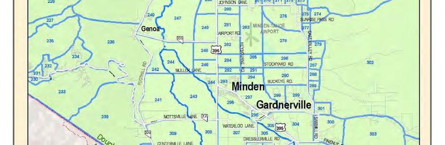
12 Figure 2-1. Douglas County and Carson City Transportation Analysis Zone (TAZ) Map 6

13 5 Douglas County/Carson City Regional Travel Demand Model Table 2-2. Douglas County/Carson City Socioeconomic Data for 2005 Jurisdiction ID POP DU OCC DU TOT EMP HOTEL OFFICE INDUS Carson City 1 58,016 24,852 23,490 26,059 2,213 12,636 5,359 Douglas County 2 51,948 24,490 20,610 19,563 6,954 4,857 3,630 Total 109,964 49,342 44,100 45,622 9,167 17,493 8,989 Jurisdiction ID RETAIL NON RETAIL ELE & MIDDLE SCHOOL HIGH SCHOOL COLLEGE Carson City 1 5, ,695 2,574 3,151 Douglas County 2 3, ,144 1, Total 9, ,839 4,359 3, EXTERNAL GATEWAY LOCATION EXTERNAL GATEWAY LOCATION 1 U.S. 50 east of Carson City 2 1. Goni US 50 Road EAST north OF CARSON of Carson CITY City 2. GONI ROAD NORTH OF CARSON CITY 3 U.S. 395 north of Carson City 3. US395 NORTH OF CARSON CITY 4 4. Highway HWY NORTH north OF of CARSON Carson City CITY 5 5. U.S. US50 50 WEST west OF of Carson CARSON City CITY 6 6. Highway HWY SOUTH south OF of DOUGLAS Douglas COUNTY County 7 7. U.S. US 395 SOUTH south of OF Douglas DOUGLAS County COUNTY 7 Figure 2-2. External Gateway Locations for the Travel Demand Model 7

14 3. HIGHWAY NETWORK Network Development Transportation Analysis Zones and Highway Geographic Database Both the highway network and the transportation analysis zones (TAZ) are based on a 331 zone structure. Of these zones, zone numbers 1 to 7 are external zones and zone numbers 8 to 331 are internal zones. The TAZ geography is included as a TransCAD geographic database in the model. However, this database is not used in any model run. The TAZ geography exists so that users can link model inputs and outputs (e.g. demographics and output trips) to the files and view results geographically. TransCAD uses the zone network in conjunction with the highway network to assign trips from the zones to the highways. The highway network is represented as a GIS geographic file. Both the attributes and the geography of the network are maintained in the TransCAD GIS. The geographic file uses shaping between nodes to accurate define both the true geography and true distances of the network links. The geographic shape of the street segments are derived from the Carson City and Douglas County GIS streets file, aerial images and TIGER/Line files. Network attributes include roadway classification type, area classification types, segment lengths and other road design-based attributes which are used for classification of free-flow speeds and capacities. Another set of attributes are free flow speed, alpha, beta and capacity exceptions for individual links, which can be used to override the default values that are applied on a global basis. These values are variables used in the trip distribution equations. A full listing of the network attributes is listed in Table

15 Table 3-1: Network Attributes FIELD_NAME DESCRIPTION ID * unique Link Identification Number Length * Length of the link in miles Dir * one-way or 2-way links ( Dir 0 = 2-way link, Dir 1 = 1-way link) NAME * Street Name FTYPE_NUM * Integer form of the Functional Class of a link FTYPE_NAME * Type of Functional Class ATYPE_NUM * Integer form for Area Type ATYPE_NAME * Description of Area Type (i.e. suburban, rural, etc.) AB_LANES * Number of Lanes on AB Direction of Link BA_LANES * Number of Lanes on BA Direction of Link UNIT * Must have a Value of 1 DAY_LANE_CAP Daily Capacity per Lane HOUR_LANE_CAP Hourly Lane Capacity AB_SPEED Free-flow Speed on AB Direction of Link (mi/hr) BA_SPEED Free-flow Speed on BA Direction of Link (mi/hr) ALPHA BPR Coefficient BETA BPR Exponent ALT_BETA Alternative BPR Coefficient for a link ALT_CAP Alternative Capacity for a link ALT_SPEED Alternative Speed for a link AB_TIME Free Flow Travel Time in AB Direction of Link (computed as Length/AB_SPEED * 60) BA_TIME Free Flow Travel Time in BA Direction of Link (computed as Length/BA_SPEED * 60) AB_TIME_PK For First Iteration =*Time, else time is AMPEAK BA_TIME_PK For First Iteration =*Time, else time is AMPEAK AB_TIME_OPK For First Iteration =*Time, else time is OFFPEAK BA_TIME_OPK For First Iteration =*Time, else time is OFFPEAK AB_TIME_AVG For First Iteration =*Time, else Weighted Average of (AMPEAK, PMPEAK & OFFPEAK) BA_TIME_AVG For First Iteration =*Time, else Weighted Average of (AMPEAK, PMPEAK & OFFPEAK) AB_HR_CAP One Hour Link Capacity BA_HR_CAP One Hour Link Capacity AB_10HR_CAP Offpeak Capacity is equal to 10* Hour Link Capacity BA_10HR_CAP Offpeak Capacity is equal to 10* Hour Link Capacity AB_DAY_CAP Daily Link Capacity BA_DAY_CAP Daily Link Capacity AB_COUNT_AM ** am peak hour Counts BA_COUNT_AM ** am peak hour Counts AB_COUNT_PM ** pm peak hour Counts BA_COUNT_PM ** pm peak hour Counts AB_COUNT_OP ** offpeak period Counts BA_COUNT_OP ** offpeak period Counts AB_ALLCOUNT ** Daily Counts BA_ALLCOUNT ** Daily Counts INCLUDECOUNT ** 1 indicates link will be used for comparisons of count to peak/offpeak hour traffic volumes INCLUDEALLCOUNT ** 1 indicates link will be used for comparisons of count to daily traffic volumes SCREENLINE ** 1 indicates the link will be used for hourly count calculations SCREENLINEALL ** 1 indicates the link will be used for daily count calculations JURISDICTIONS Jurisdiction boundaries KFACTOR_DISTRICTS kfactor districts based on links Field names denoted with a * are required fields for the model. Field names denoted with a ** are required only in the model option that compares count information with model flow results. 9

16 The highway network also contains traffic counts compiled by Parsons that were obtained primarily from NDOT. Both hourly and daily 2005 base year Annual Average Daily Traffic (AADT) counts were based on traffic counts taken during 2003, 2004 and This data was entered into the highway network input files for model validation, providing a comparison between counts and model forecasts. For more information, see page A-1 of Appendix A in the traffic model report. All hourly counts are based on 2003/2004 estimates and only weekday counts were included. In cases where more than one count existed on the same roadway segment, an average count was calculated. In other cases where a line segment had both hourly and AADT counts, the hourly counts were factored to the AADT count since it was assumed that AADT counts are more accurate. Node Attributes In TransCAD, nodes are an additional layer in the highway geographic database with unique ID s and optional attribute fields. In the Travel Demand Model, the first 331 node IDs are designated as the centroids. There is also a field in the nodes called TAZ that has the traffic analysis zone number for centroids nodes. Highway Network (.NET) Creation From this line geographic file, a TransCAD network is created. The network uses the fields LENGTH, FTYPE_NUM, *TIME, *_HR_CAPACITY, *10HR_CAPACITY, ALPHA, and BETA. Centroids have also been set in this network. The model includes a button that automatically recreates the highway network. The model also has a supplementary input file (speed-capacity lookup table), which is used to help create the network. The values of this speedcapacity lookup table are documented in Tables 3-2 and 3-3. Table 3-4 represents the crossclassification lookup value for the Facility and Area types Table 3-2: Hourly Capacities (vehicles per hour per lane) Used for the Travel Demand Model Area Types Functional Class Central Business District (CBD) Urban Rural System ramps 2,000 2,000 2,000 Minor arterials Major arterials Ramps 1,600 1,600 1,600 Interstates 2,000 2,000 2,000 Freeways 2,000 2,000 2,000 Expressways 1,100 1,200 1,400 Collectors Externals 99,999 99,999 99,999 10

17 Table 3-3: Free-Flow Speeds (miles per hour) Used for the Travel Demand Model Area Type Functional Class CBD Urban Rural System ramps Minor arterials Major arterials Ramps Interstates Freeways Expressways Collectors Externals Table 3-4: Facility Type and Area Type Classification in the Travel Demand Model Functional Class Facility CBD Urban Rural System ramps Minor arterials Major arterials Ramps Interstates Freeways Expressways Collectors Centroids Externals The speed-capacity lookup table automatically fills in link speeds, hourly and daily lane capacities and link alpha and beta values by functional classification and area type. By matching up the FTYPE_NUM and ATYPE-NUM fields in the network with this lookup table, the model automatically fills in the following fields: DAY_LANE-CAP, HOUR_LANE_CAP, AB_SPEED, BA_SPEED, AB_TIME, BA_TIME, ALPHA, BETA, AB_HR_CAP, BA_HR_CAP, AB_10HR_CAP, BA_10HR_CAP, AB_DAY_CAP and BA_DAY_CAP. The model also uses the fields AB_LANES, BA_LANES and UNIT as inputs network fields. Appendix A describes all of the fields in this table. Turn Penalties Table A turn penalties file is also included within the model stream. The turn penalties file is based on nodes and reflects, on a from-link to to-link basis, prohibitions and delays from certain turn movements from occurring during the traffic assignment process. The turn penalties are embedded into the network during network creation and affect the highway skimming and highway assignment sections of the model. Skim is a unit of measurement (time, distance, cost, etc.) between two TAZ. The following table describes the fields of the table: Turn Penalties Table (xx_turn-prohib.bin)* 11

18 Base Year Network Road Classification Figure 3-1 illustrates the classification of roadways coded in the Year 2005 Highway Network. The roadway network was developed from scratch using the TIGER files as a starting point and refining the roadway classifications as appropriate. This roadway network along with the roadway classification was used for the model development and validation purposes. The centroids are not plotted in this figure to allow better visibility of the roadway network BASE NETWORK 2005 BASE NETWORK Roadway Roadway Classification Classification Externals Minor Major Freeway Expressway Collector Centroids Externals Minor Major Freeway Expressway Collector Figure 3-1: Year 2005 Douglas County and Carson City Highway Network 12

19 Highway Skims Once the highway network is created, the model performs highway skims from centroid node to centroid node. The travel time is minimized and travel distance is skimmed. Both the offpeak and peak travel periods (8:00 9:00 a.m. and 5:00 6:00 p.m.) are skimmed as input to the downstream models. To calculate the offpeak skims, free-flow travel times are used, which are derived from the formula: GIS Length/Free-Flow Speed * 60. To calculate the peak skims, congested travel times are used. Congested travel times are calculated from the output of previous traffic assignments and are described in more detail in the Assignment section of this document. After the peak and offpeak travel time matrices are calculated, intrazonal travel times are calculated and then origin and terminal times are added to them. The procedure used for calculating intrazonal travel times was the closest neighbors approach. For each row origin, the travel time to its two closest neighbors is found from the matrix. The intrazonal time is computed as one half of the travel time to its closest neighbor. After intrazonal travel times are estimated, additional origin and terminal times of 4 minutes are added to the skim matrix. The highway skims proceed in the following manner: 1. The highway database and network are opened and nodes that are centroids are selected. 2. A travel time matrix from centroid to centroid is calculated using the peak and offpeak skims. 3. Intrazonal times taking into account nearest adjacent neighbor times are calculated. 4. Origin and terminal times are added to the matrix. Descriptions of the input and output files and parameters can be found in Appendix A. 13

20 4. TRIP GENERATION Resident Model Set Overview The resident trip generation models that were recently estimated and calibrated for the Clark County area were used as the starting point for the trip generation and calibration. The trip production models are cross-classification models stratified by income group and household size. In effect, the models provide trip production rates by trip purpose for each household size, income group stratum. The independent variable used is the number of households in the stratum. Five household size strata are used: 1 person households 2 person households 3 person households 4 person households 5 or more person households The travel model uses four household income groups, consistent with the 2000 U.S. Census income categories. All incomes are represented in 1999 dollars: Low income (Less than $19,999) Lower-middle income ($20,000 to $29,999) Upper-middle income ($30,000 to $49,999) High income ($49,999 or more) It is necessary to estimate a joint distribution of households by income group and household size (i.e., 20 separate cells) for each TAZ. Submodels (documented below) are provided to produce these data from normal socioeconomic information forecast for each TAZ: population in households, number of households, and median income. As income increases, the rate of auto ownership and trip generation increases. The trip attraction models are cross-classification-like models with number of employees by employment by type and households being the explanatory variables. The employment and household data are normally forecast by TAZ. The resident trip generation models have been developed for the following trip purposes: Home-Based Work (HBWork) 14

21 Home-Based School (HBSchool) Home-Based Shop (HBShop) Home-Based Other (HBOther) Non-Home-Based (NHB) All trip rates documented herein are based on total person trips made in motorized vehicles. Person trips made using non-motorized modes such as walk, wheelchair, or bicycle and person trips made using unspecified modes were not included in the data used to estimate the trip rates. Socioeconomic Submodels Socioeconomic submodels were developed from 2000 Census data to estimate the number of households by income group and household size for each TAZ. Three submodels were developed: A submodel to estimate the number of households by household size based on the average household size of the TAZ and the number of households in the TAZ. A submodel to estimate the number of households by income group based on the ratio of the median income for the TAZ to the regional median income and the number of households in the TAZ. A submodel to estimate the joint distribution of households by income group and household size based on the results from the above two submodels Base Year Data The 2005 base year data for Douglas County and Carson City were estimated based on Year 2000 Census information. Table 4-1 shows the summary of the household information. The information for persons per household and number of households in certain income ranges was extracted from the dataset, which contained 64 block groups. The block group data have been used to estimate household size and income group submodels for use in the trip generation modeling process. The regional median income is based on the 2000 U.S. Census information for both Douglas County and Carson City. This data reveals that one-half of the households have an income less than $44,448 and the other half of the households have an income above this figure. The household population includes everybody living in the household regardless of their age. Table 4-1 has been revised to clarify the total households in both subsets. Table 4-1: Douglas County and Carson City 2005 Data Summary Category Units Population 109,964 1 person households 9,010 2 person households 14,055 3 person households 5,700 4 person households 4, person households 3,154 Total occupied households 36,665 Households with income less than $19,999 6,472 Households with income between $20,000 and $29,999 4,374 Households with income between $30,000 and $49,999 8,893 Households with income greater than $49,999 16,926 Total occupied households 36,665 Regional median income $44,488 15

22 The Households Size Disaggregation and Household Income Disaggregation Submodels were borrowed from the 2004 Las Vegas RTC Travel Demand Model recently developed by Parsons for the Las Vegas metropolitan area. This model also used data from the existing Carson City model. The joint distributions of households by household size and household income was, however, calibrated to the 2000 Census information for the counties of Douglas and Carson City. Households by Household Size Disaggregation Submodel The hypothesis underlying the household size disaggregation model is that for any given zonal average household size (i.e., persons per household) there is a specific mix of households for each integer household size (i.e., one person households, two person households, etc.). In order to implement this hypothesis as a functional model, household data from the 2000 Census were summarized and grouped by average household size. This summarization was performed at the census block group level with data grouped by ranges of 0.1 persons per dwelling unit (for example, 1.0 to 1.04 were grouped to the 1.0 range, 1.05 to 1.14 were grouped to 1.1, 1.15 to 1.24 were grouped to 1.2, etc.). The summarized data showed a reasonable relationship between average household size and the distribution of the integer persons per household when they were plotted. A preliminary model was developed by hand-fitting curves to the census data. These nonlinear, hand-fitted curves were not an adequate model since the percent of integer households did not necessarily meet two essential criteria. These two criteria were: The sum of the integer household percents equal for each average household size The average persons per household calculated from the integer household percents equal the average household size being used as the independent variable. Each average household size range was investigated to ascertain the change required in the integer household size percents to meet the above two criteria. The curves were then redrawn and smoothed to produce a usable household size disaggregation model. The final model is shown in Figure 4-1 and Table 4-2. Percent of Households PCT1 PCT2 PCT3 PCT4 PCT Average Household Size Figure 4-1: Household Size Disaggregation Submodel 16

23 Table 4-2: Household Size Disaggregation Submodel Input Average Proportion of Households by Size Household Size 1 Person 2 Person 3 Person 4 Person 5+ Person Sum 1 Implied Average Household Size Average household sizes for five or more person households used to estimate the implied average household size: Input Household Size Range Average 5+ Household Size or more

24 Households by Income Group Disaggregation Model The income group disaggregation model is similar in form to the household size disaggregation model. The independent variable for the model is the ratio of the TAZ median income to the regional median income. The model was estimated using block level data from the 2000 Census. The income ranges defined by the Census for the block group data that was used for the income group disaggregation model are shown in the Table 4-3. The regional median income in 1999 dollars and median incomes for each of the block groups were also obtained from the block group data. Table 4-3: Household Income Classification Income Group 2000 Census Income Range Households in Range (2000 Census) Used (1999 Dollars) Number Percent Low Less than $19,999 6, % Lower-middle $20,000 $29,999 4, % Upper-middle $30,000 $49,999 8, % High $50,000 or more 16, % For future forecasts, median incomes can be left unchanged in stable TAZs. For TAZs that are developed or redeveloped between the base and forecast years, TAZ median incomes can be estimated from similar TAZs. Future year income forecasts can be in 1999 or future year dollars. The effect of changing the base year for income forecasts will be accounted for by using the ratio of the TAZ median income to the regional median income. In effect, the income group disaggregation model is self-correcting for changes in real or inflationary income. The ratios of the TAZ median incomes to the regional median income and the proportions of households in each of the four income groups were calculated for each block group. Four curves were then developed for the income group disaggregation submodel to represent the proportions of households within the income ranges for each value of the income ratio. The proportions defining the curves were constrained to sum to 1.0 for each value of the income ratio. In addition, the curves were defined such that the implied TAZ median income would fall in the income group implied by the input income ratio. For example, if the input TAZ median income is $31,200, the TAZ to regional median income ratio is 0.7. The income group disaggregation model, a total of 48.1 percent of the households would have incomes in the low and lower-middle income group ranges. The lowest 5.96 percent of the 31.9 percent of the households in the uppermiddle income range (i.e., 1.9 percent of all households in the region) would also have incomes less than $31,200. If incomes in the upper-middle income range are assumed to be uniformly distributed (an unlikely case), the implied median income for the TAZ would be 5.96 percent of the range from $30,000 $49,999, or $31,192. Table 4-4 and Figure 4-2 show the income group disaggregation model. 18

25 Table 4-4: Income Group Disaggregation Submodel 1 Input Income Ratio Proportion of Households by Income Group Low Income Lower-Middle Income Upper-Middle Income High Income Total Implied Median Income Implied Income Ratio , , , , , , , , , , , n/a 1 n/a n/a 1 n/a n/a 1 n/a n/a 1 n/a n/a 1 n/a n/a 1 n/a n/a 1 n/a n/a 1 n/a n/a 1 n/a n/a 1 n/a n/a 1 n/a n/a 1 n/a n/a 1 n/a n/a 1 n/a n/a 1 n/a n/a 1 n/a n/a 1 n/a n/a 1 n/a n/a 1 n/a n/a 1 n/a n/a 1 n/a n/a 1 n/a n/a 1 n/a n/a 1 n/a n/a 1 n/a n/a 1 n/a n/a 1 n/a n/a 1 n/a n/a 1 n/a n/a 1 n/a n/a 1 n/a n/a 1 n/a n/a 1 n/a n/a 1 n/a n/a 1 n/a n/a 1 n/a n/a 1 n/a 1 Since the median income falls in the high income group and the maximum income for that group is undefined, the implied median income cannot be estimated. 19

26 100% 90% Percent of Households 80% 70% 60% 50% 40% 30% 20% 10% PCT1 PCT2 PCT3 PCT4 0% Income Ratio Figure 4-2: Income Group Disaggregation Submodel Estimating Joint Distributions of Households by Socioeconomic Strata The two submodels described in the previous sections result in preliminary estimates of the following univariate, or marginal, distributions of households for each TAZ: Households by household size Households by income group The initial applications of the models result in preliminary estimates for the following reason. If the households are summed over the strata included in each univariate distribution for each TAZ, the total will be the number of households for the TAZ. For example, if the estimated households by household size are summed for TAZ 1, the total will be the number of households in TAZ 1. To ensure that the regional sums match, a marginal weighting, or fratar, process can be applied on a regional basis. For this application, the input matrices are the estimates of households for each TAZ in the region from the preliminary applications of the household size or income group disaggregation submodels. The marginal distributions for this application of the marginal weighting process are the total numbers of households for each TAZ and the estimated regional households for the socioeconomic stratum being factored regional households by household size or regional households by income group. The results of this marginal weighting step will ensure that the total numbers of households for each TAZ are correct when the various socioeconomic distributions are summed by TAZ, and that the regional households by socioeconomic stratum are correct when the households for the stratum are summed across all TAZs. Regional distributions of households by income group and household size are used to develop the regional control totals for households. A third submodel completes the disaggregation and results in estimates of households jointly stratified by income group and household size for each TAZ. The submodel uses the results from the modified marginal distributions of households by income group and households by household size for each TAZ along with the regional joint distribution of households by income group and 20

27 household size (Tables 4-5 and 4-6). The final joint distributions are shown in Tables 4-5 and 4-6 and were developed by updating the joint distributions that was developed for Clark County. The Clark County joint distribution is based on the Public Use Micro Sample (PUMS) data from the 2000 Census, which is a one percent sample of all households for a given county. The Clark County estimates for the joint distribution was then fratared to match the marginals that were obtained for the 2000 Census for Douglas County and Carson City by household size and income group. The median income for each TAZ was derived from the 2000 Census block group data and is represented in 1999 dollars. Table 4-5: Households by Income Group and Household Size Household Size Income Group Total Low 3,689 1, ,472 Low-middle 1,483 1, ,374 Upper-middle 2,269 2,654 1, ,893 High 1,569 7,163 3,234 2,981 1,979 16,926 Total 9,010 14,055 5,700 4,746 3,154 36,665 Table 4-6: Proportion of Households by Income Group and Household Size Household Size Income Group Total Low 10.1% 4.0% 1.7% 1.1% 0.7% 17.7% Low-middle 4.0% 4.8% 1.4% 1.1% 0.6% 11.9% Upper-middle 6.2% 10.0% 3.6% 2.7% 1.9% 24.3% High 4.3% 19.5% 8.8% 8.1% 5.4% 46.2% Total 24.6% 38.3% 15.5% 12.9% 8.6% 100.0% The third submodel effectively fratars the regional joint distribution of households by income group and household size on a TAZ-by-TAZ basis to match the modified marginal distributions of households by income group and households by household size for each TAZ. All three submodels have been coded in TransCAD GISDK scripts for automatic application each time the trip generation module is invoked. Socioeconomic Model Application Summary In summary, the process for estimating the number of households for the joint distribution of households by income group and household size for each TAZ makes extensive use of the marginal weighting technique. The process is as follows: Preliminary estimates of the number of households by income group and households by household size are developed for each TAZ using the appropriate socioeconomic disaggregation submodel. 21

28 The preliminary estimates of households for each marginal socioeconomic distribution for each TAZ are marginally weighted so that the numbers of households for each TAZ and the total numbers of households for each socioeconomic group for the region are matched. The regional distribution of households by income group and household size are marginally weighted to match the estimated marginal distributions of households by income group and household size on a TAZ-by-TAZ basis. All three submodels have been coded in TransCAD GISDK scripts for automatic application each time the trip generation module is invoked. Trip Production Models Trip production models were borrowed from the Las Vegas region and were estimated using a traditional cross-classification analysis. Purpose specific person trips made in motorized vehicles were summarized for each household and average trip rates per household were then calculated for all households within defined socioeconomic strata. As outlined in the socioeconomic data section above, two household characteristics, household size and income group, were used to define the household strata. As income becomes greater, the rate of auto ownership and trip generation generally increases. However, larger household size causes a greater increase in trip generation rates than rising income levels. These submodels were further refined to better represent Douglas and Carson City. Home-Based Work Trip Production Model Table 4-8 shows the Home-Based Work trip production model for the region. Based on strict statistical comparisons of trip rates, some combining of cells could have been performed. However, the increase in trip rates as household size increased and as income group increased was very reasonable. Table 4-8: Home-Based Work Trip Production Model Household Size Income Group Low Lower-middle Upper-middle High Home-Based School Trip Production Model Table 4-9 shows the HBSchool trip production model for the region. Shading of cells shows the trip rate combinations performed as part of the model estimation. The HBSchool trip production model shown in Table 4-9 is for trips made in motorized vehicles to all: Pre-schools and kindergartens Elementary schools, middle schools, and high schools Community colleges and vocational/technical schools. 22

29 Table 4-9: Home-Based School Trip Production Model Household Size Income Group Low Lower-middle Upper-middle High The trip rates shown in Table 4-9 tend to vary more by household size than by income group. This is logical since HBSchool trips are primarily dependent on the presence of school-age children in a household, which should be highly correlated with household size. The very low rate for one-person households reflects a small number of single person households where the householder is a student. The difference between trip rates for low and lower-middle income, two person households probably reflects the impact of single-parent households. Specifically, low income, two-person households are probably more likely to be single parent with a child households, while two (working) adults are more likely to comprise two-person, lower-middle and upper-middle income households. The HBSchool trip production model shown in Table 4-9 has sensitivity to household structure. In other words, since the model is stratified by household size, it is sensitive to changes in household size the increase or decrease in number of children in a household. Nevertheless, the total HBSchool productions should be compared to the total attractions based on enrollment projections. If a large imbalance is noted, an inconsistency between forecast population and households, and forecast school enrollment is possible. Since only person trips made in motorized vehicles have been summarized in the trip rates shown in Table 4-9, behavior regarding the propensity to walk or bicycle to school is assumed to remain constant over time. This assumption is consistent with the assumption made when HBSchool trip attractions are forecast based on school enrollment. Home-Based Shop Trip Production Model Table 4-10 shows the HBShop trip production model for the region. Shading of cells shows the trip rate combinations performed as part of the model estimation. Again, the trip rates tend to vary by household size, but not income group, and for this purpose, the variation in trip rates across two-, three-, and four-person households was not significant. The lack of variation across income groups is generally logical. Households need to shop for basic necessities regardless of income. Income is a primary determinant of whether shopping takes place at a high-end retail store or a discount store. Table 4-10: Home-Based Shop Trip Production Model Household Size Income Group Low Lower-middle Upper-middle High

30 The lack of variation across household size is also reasonable. The two-person household rate is about twice the one-person household trip rate, reflecting an increased tendency for both household members to shop together. However, for three- and four-person households, no significant increase in the trip rate was observed. This reflects the fact that, quite often, not all household members are required for the shopping trip. In a three- or four-person household, this would indicate the tendency for only one extra household member to participate in the shopping trip. Home-Based Other Trip Production Model Table 4-11 shows the HBOther trip production model for the region. Shading of cells shows the trip rate combinations performed as part of the model estimation. The variation in trip rates across household sizes is reasonable. In addition, some variation in trip rates across income groups might reflect the influence of additional disposable income, allowing for additional trips to be made (see also the NHB trip rates). Table 4-11: Home-Based Other Trip Production Model Household Size Income Group Low Lower-middle Upper-middle High Non-Home-Based Trip Production Model Table 4-12 shows the NHB trip production model for the region. Shading of cells shows the trip rate combinations performed as part of the model estimation. The variation in trip rates across household sizes is reasonable. In addition, the variation in trip rates across income groups probably reflects the influence of additional disposable income allowing for additional trips to be made (see also the HBOther trip rates). The NHB trip production model is applied only to obtain a regional control total for NHB trips. The locations of the actual trip productions are determined using an allocation model. For the Douglas County and Carson City region, the NHB trip attraction model is used as the allocation model (in effect, NHB productions are set equal to NHB attractions on a TAZ-by-TAZ basis after the NHB attractions are scaled to match the regional total NHB productions). Table 4-12: Non-Home-Based Trip Production Model Household Size Income Group Low Lower-middle Upper-middle High

31 Trip Attraction Models The trip attraction models were borrowed from the Las Vegas region and were estimated using an aggregate cross-classification analysis coupled with some guiding principles. The aggregate cross-classification technique was implemented by aggregating expanded trip attractions by the type of land use at the attraction end of the trip. Thus, if a person traveled from home to a store to shop and then traveled back home again, two HBShop attractions were shown at a retail land use. Once total attractions by land use have been aggregated by land use, they are divided by the total employment (or households in the case of residential land uses) associated with the land use. Table 4-13 shows the land use types along with the associated type of employment or households used as the independent variable. While it is not possible to estimate any calibration statistics using this procedure, it has proved very successful in producing reasonable trip attraction models in other regions. It is not affected by the high correlation between the explanatory variables (e.g., employment by type) that typically plagues trip attraction models estimated using district-based linear regression techniques. Table 4-13: Land Use Types and Explanatory Variables for Trip Attraction Rates Land Use Type Explanatory Variable Residential Basic industries including forestry, fishing, mining, manufacturing, public utilities, warehousing Retail Recreational and personal services including theaters, schools, government, convention centers, daycare, sports facilities and gyms Churches and other religious facilities Medical facilities Banks Personal and business services including financial, insurance, and real estate, consultants, attorneys, accountants Casinos and hotels Unknown Parks and open spaces Households Industrial employment Retail employment Office and other non-classified employment Casino and hotel employment None One guiding principle used in the estimation of trip attraction rates was that the explanatory variables had to be logical attractors of trips for the purpose being modeled. Thus, all home-based school trip attractions were assumed to occur at schools with the explanatory variable being school enrollment. Likewise, all home-based shop trip attractions were assumed to be made to retail establishments with retail employment being the explanatory variable. Table 4-14 summarizes the trip attraction models. All rates shown in Table 4-14 are for person trips made in motorized vehicles. The following sections provide brief discussions of the trip attraction models. 25

32 Table 4-14: Trip Attraction Models Regular Trip Attraction Rate per Employment School Enrollment Trip Purpose Trip Attraction Rate per Household Industrial Office and Non-Classified Retail Casino Hotel Total Grades 1 8 Grades 9 12 Grades 13+ Special generators - Casino HBWork HBSchool HBShop 2.37 HBOther Non-HB Home-Based Work Trip Attraction Model There are two items of note in the HBWork trip attraction model. First, there is a low HBWork trip attraction rate per household. While it might have been possible to specify that HBWork trips would be attracted only to establishments with employment, the low attraction rate per household is similar to that found in a number of other cities. The rate probably accounts for domestic help and service calls (e.g., insurance agents, plumbers, and large appliance repair personnel) made directly from the employee s home to a residential worksite. The HBWork trip productions will be output by income group in an effort to improve trip distribution modeling, and when a mode choice model is added to the modeling process, mode choice. Since the HBWork trip attraction model has not been stratified by income group, the total HBWork attractions will be scaled to match total productions for each of the four income groups in question. Such a procedure results in a trip attraction model that assumes that the same proportions of trip attractions by income group hold constant across all TAZs in the region. While such an assumption produces a gross regional average, the procedure and results are still quite effective in improving trip distribution and mode choice. Home-Based School Trip Attraction Model The HBSchool trip attraction rates vary by age of the student making the trip. The rate for elementary school-aged students (grades 1 8) is substantially lower than the rate for high school students. These rates probably reflect a higher likelihood for elementary school students to attend neighborhood schools within walking distance of the home and a higher likelihood for high school students to live farther from their schools as well as high school students capabilities of driving themselves to school. The low HBSchool trip attraction rate per enrollee in grades 13 and higher probably reflects the part-time nature of those trips. Specifically, many students in post-high school educational institutions either attend part-time or establish their schedules so that they do not attend classes every school day. 26

33 Home-Based Shop Trip Attraction Model The HBShop trip attraction model was based on the assumption that all shop trips are attracted by retail employees. Based on the summary of the household survey data, numerous shop trips were made to non-retail land uses. Undoubtedly, this happened in some cases a trip for shopping purposes might have been made to a retail establishment at a casino (listing the casino as the destination), a person could have stopped at a beauty salon to purchase hair care products, or a could have stopped at someone s home to pick up goods from an in-home business. In some cases (e.g., the shopping trips to the beauty salon or the home), shopping trips are truly made to land uses with no retail employees. However, these unadjusted HBShop rates for non-retail were very small (0.01 trips per employee). Thus, the assumption that all HBShop trips are attracted by retail employment is reasonable. The HBShop rate per full-time equivalent retail employee might seem low 2.37 HBShop trip attractions per retail employee suggests that each retail employee serves only about 1.15 people per day. However, if HBShop, HBOther, and NHB trips per retail employee are summed, the overall attraction rate per retail employee is (NHB must be counted twice due to the method used to model NHB trips), or about 5.6 people per day. Home-Based Other Trip Attraction Model The HBOther trip attraction model includes rates for all types of employment and for households. The travel demand model attracts 0.38 HBOther person trips per household. In essence, this suggests that, on the average, about one out of every five homes has a visitor during the day. Thus, the travel demand model focuses HBOther attractions more toward employment areas than toward residential areas. Non-Home-Based Trip Attraction Model Like the HBOther trip attraction model, the NHB trip attraction model includes rates for all types of employment and for households. Continuing the example of trips attracted per household, the travel demand model attracts 0.2 NHB trips per day. Since NHB productions are set equal to NHB attractions on a TAZ-by-TAZ basis after balancing to the regional control total for NHB trips estimated using the household-based trip production model, each home attracts an average of 0.2 visitors per day. Combined with the HBOther rates, the travel demand model suggests that each home has 0.4 visitors per day, or in other words, every 2.5 homes has a visitor each day. Special Generator Trip Attraction Models The trip attraction model includes unique trip attraction rates for casinos and is considered as special generator with the ability to have unique trip attraction rates per employee. The special generator models simply affect the total trip attractions to these locations. It must be noted however that the special generators are not currently being used but are provided as part of the model development and can be used without any changes to the model structure. 27

34 5. TRIP DISTRIBUTION Introduction Trip distribution assigns the trips calculated during trip generation to the appropriate production and attraction TAZ pairs. The trips to each TAZ pair are determined based on the gravity model. T ij = P i n k = 1 K F A ij ij j ( ) K F A ik ik k where: T ij = trips between zone i and zone j P i = productions in zone i A j = attractions in zone j K ij = K-factor adjustment between zone i and zone j F ij = friction factor between zone i and zone j i = production zone j = attraction zone n = total number of zones The calibration process calculates the friction factors and K-factors used in the above equation. The goal in calibrating trip distribution is to arrive at friction factors and K-factors such that the average trip lengths and trip length frequency distributions resulting for each trip purpose are similar to those from survey data. 28

35 Gamma Function The friction factors used in the Douglas County/Carson City Travel Demand Model are based on a gamma function. This type of function has three parameters alpha (a), beta (b), and gamma (c) as shown in the following equation. F = a t e ij b ij ct ij where: F ij = friction factor between zone i and zone j t ij = travel time between zone i and zone j a = alpha parameter b = beta parameter c = gamma parameter This document adheres to the above equation in defining the three parameters. TransCAD, however, requires the values of beta and gamma to be of the opposite sign when defining the parameters. The values input into the TransCAD model script for beta and gamma are opposite the values listed in this document. The gamma function is a smooth, monotonically decreasing function when both the beta and gamma parameters are negative. This suggests that travelers are sensitive to travel time as they travel to satisfy their needs. For example, a person is less likely to travel to a grocery store ten minutes from home if there is a store only five minutes from home. If the calibrated beta parameter is positive, the function increases to an inflection point and then decreases as the travel time increases. In general, this should be avoided, since it implies that up to a certain point, travelers have a desire to travel further to satisfy their need for travel. In certain cases, a positive beta parameter can be justified. If the calibrated gamma parameter is positive, the function decreases to a point and then increases. A positive gamma parameter can be used if the inflection point is greater than the highest travel time expected between any two points in the region. Alternatively, the function can be converted to a look-up table and modified to be equal to the minimum value at travel times greater than the inflection point. Source of Data The work trip length frequency distribution from the 2000 Census was obtained for Douglas County and Carson City. This observed data was used to compare the modeled trip length frequencies. Calibration Process The trip distribution calibration process included determining the parameters for the friction factors and calculating the K-factors if needed. K-factors are calculated to adjust for major distribution characteristics not explained by travel time. These differences may be caused by natural or manmade barriers, such as rivers or railroads, or by socioeconomic characteristics. The 29

36 first process was to determine the friction factor parameters. After the friction factors were finalized, it was found that there was no need to calculate K-factors. The K-factors procedures are provided as part of the model development process but were not used Friction Factor Parameters The following list explains the general process taken for each trip purpose to calculate the friction factors. Run the model with reasonable set of friction factor parameters obtained from another region. Compare histograms and average trip lengths of the results of the model run with the observed data. Based on the results of the comparisons, calculate the desired friction factors for a new model run that would more closely match the observed trip length frequency distribution. Use linear regression techniques (based on a log-transformation of the gamma function) to convert the desired friction factors into revised gamma function parameters for use in TransCAD. Run the model with the new gamma function parameters and continue with the comparisons and calculations of new gamma parameters until the results compare reasonably with the observed data. Calibrated gamma function parameters for home-based work trips are shown in Table 5-1 and Figure 5-1 shows the gamma functions. Table 5-1: Final Friction Factor Parameters Home-Based Work Parameter HBW Income 1 HBW Income 2 HBW Income 3 HBW Income 4 Alpha 1,064,931 1,064,931 1,064,931 1,064,931 Beta Gamma Format Function Function Function Function 1.E+06 HBW - Income E+05 Friction Factors 1.E+04 1.E+03 1.E+02 1.E+01 1.E Time (minutes) Figure 5-1: Friction Factor Parameters Home-Based Work 30

37 Table 5-2 and Figure 5-2 show the friction factors for other resident trip purposes. The gamma parameter is positive for the home-based shop and home-based other trip purposes. The homebased shop gamma function begins increasing after about 80 minutes of travel time and the homebased other function begins increasing after about 60 minutes of travel time. For the non-homebased and home-based other trip purposes, the gamma function was converted to a tabular form for use in TransCAD. The friction factors for travel times greater than the times at the inflection points were modified to be equal to the minimum value of the gamma function. Table 5-2: Final Friction Factor Parameters Other Trip Purposes Parameter HBSchool HBShop HBOther NHB Alpha 1,136,464 1,185,375 1,072, ,402 Beta Gamma Format Function Function Table Table 1.E+06 1.E+05 1.E+04 HBSchool HBOther HBShop NHB Friction Factors 1.E+03 1.E+02 1.E+01 1.E+00 1.E-01 1.E E-03 1.E-04 Time (minutes) Figure 5-2: Friction Factor Parameters Other Trip Purposes Trip Length Frequency Distributions The travel time comparison of Home based work trips with the 2000 Census information is shown in Figure 5-3. It can be seen that the observed and the modeled travel times are very similar. The trip length frequency distributions are based on trip duration (time) using 5 minute bins to categorize the data. Table 5-3 summarises the travel time results for all the Home-based work trip purposes The trip length (distance) for Home Based work trip purposes is shown in Figure 5-4 and uses 0.25 mile bins to categorize the data. In other words, the bin for 5 minutes represents all trips in the range 5.0 to 9.99 minutes; the bin for 0.25 mile includes all trips in the range 0.0 to 0.25 miles. 31

38 Although no information was available for other trip purposes from the 2000 census, the travel times and trip distances for these other trip purposes are within acceptable limits. Figures 5-5 to 5-8 and the Table 5-4 summarizes the results for the non work trip purposes VALIDATION - TRAVEL TIME COMPARISONS (HOME BASED WORK) 30% 25% CENSUS MODEL-FINAL PERCENTAGE IN EACH INTERVAL 20% 15% 10% 5% 0% < 10 MIN MIN MIN MIN MIN MIN MIN TRAVEL TIME IN MINUTES MIN MIN Figure 5-3: Travel Time Frequency Distributions Home-Based Work Trips >90 MIN 2005 VALIDATION - TRIP LENGTH DISTRIBUTION (HOME BASED WORK) PERCENTAGE IN EACH INTERVAL 30% 2005MODEL-FINAL 25% 20% 15% 10% 5% 0% < 2.5 MI 2.5 MI - 5 MI 5 MI MI 7.5 MI - 10 MI 10 MI MI 12.5 MI - 15 MI 15 MI MI TRIP LENGTH IN MILES 17.5 MI - 20 MI 20 MI MI 22.5 MI - 25 MI Figure 5-4: Trip Length Frequency Distributions Home-Based Work Trips >25 MI 32

39 2005 VALIDATION - TRAVEL TIME DISTRIBUTION (HOME BASED SCHOOL) 12,000 10, MODEL-FINAL NUMBER OF TRIPS 8,000 6,000 4,000 2,000 - < 10 MIN MIN MIN MIN MIN MIN MIN MIN >60 TRAVEL TIME IN MINUTES 2005 VALIDATION - TRIP LENGTH DISTRIBUTION (HOME BASED SCHOOL) NUMBER OF TRIPS 10,000 9,000 8,000 7,000 6,000 5,000 4,000 3,000 2,000 1, MODEL-FINAL < 2.5 MI 2.5 MI - 5 MI 5 MI MI 7.5 MI - 10 MI 10 MI MI 12.5 MI - 15 MI 15 MI MI 17.5 MI - 20 MI 20 MI MI 22.5 MI - 25 MI >25 MI TRIP LENGTH IN MILES Figure 5-5: Home-Based School Trips Frequency Distribution 33

40 2005 VALIDATION - TRAVEL TIME DISTRIBUTION (HOME BASED SHOP) 18,000 16, MODEL-FINAL 14,000 NUMBER OF TRIPS 12,000 10,000 8,000 6,000 4,000 2,000 - < 10 MIN MIN MIN MIN MIN MIN MIN MIN >60 TRAVEL TIME IN MINUTES 2005 VALIDATION - TRIP LENGTH DISTRIBUTION (HOME BASED SHOP) 16,000 14, MODEL-FINAL NUMBER OF TRIPS 12,000 10,000 8,000 6,000 4,000 2,000 - < 2.5 MI 2.5 MI - 5 MI 5 MI MI 7.5 MI - 10 MI 10 MI MI 12.5 MI - 15 MI 15 MI MI 17.5 MI - 20 MI 20 MI MI 22.5 MI - 25 MI >25 MI TRIP LENGTH IN MILES Figure 5-6: Home-Based Shop Trips Frequency Distribution 34

41 2005 VALIDATION - TRAVEL TIME DISTRIBUTION (HOME BASED OTHER) 70,000 60, MODEL-FINAL NUMBER OF TRIPS 50,000 40,000 30,000 20,000 10,000 - < 10 MIN MIN MIN MIN MIN MIN MIN MIN >60 TRAVEL TIME IN MINUTES 2005 VALIDATION - TRIP LENGTH DISTRIBUTION (HOME BASED OTHER) NUMBER OF TRIPS 60,000 50,000 40,000 30,000 20,000 10, MODEL-FINAL - < 2.5 MI 2.5 MI - 5 MI 5 MI MI 7.5 MI - 10 MI 10 MI MI 12.5 MI - 15 MI 15 MI MI 17.5 MI - 20 MI 20 MI MI 22.5 MI - 25 MI >25 MI TRIP LENGTH IN MILES Figure 5-7: Home-Based Other Trips Frequency Distribution 35

42 2005 VALIDATION - TRAVEL TIME DISTRIBUTION (NON HOME BASED) 70,000 60, MODEL-FINAL NUMBER OF TRIPS 50,000 40,000 30,000 20,000 10,000 - < 10 MIN MIN MIN MIN MIN MIN MIN MIN >60 TRAVEL TIME IN MINUTES 2005 VALIDATION - TRIP LENGTH DISTRIBUTION (NON HOME BASED) NUMBER OF TRIPS 50,000 45,000 40,000 35,000 30,000 25,000 20,000 15,000 10,000 5, MODEL-FINAL < 2.5 MI 2.5 MI - 5 MI 5 MI MI 7.5 MI - 10 MI 10 MI MI 12.5 MI - 15 MI 15 MI MI 17.5 MI - 20 MI 20 MI MI 22.5 MI - 25 MI >25 MI TRIP LENGTH IN MILES Figure 5-8: Non-Home Based Trips Frequency Distribution 36

43 Table 5-3: Trip Distribution Calibration Results Home-Based Work Trips by Income Group Observed HBW Income 1 HBW Income 2 HBW Income 3 HBW Income 4 HBW - Total Average trip duration (minutes) NA NA NA NA Average trip length (miles) NA NA NA NA NA Modeled Average trip duration (minutes) * Percent difference from observed 3.15% Average trip length (miles) * Percent difference from observed * Weighted average NA = not available Table 5-4: Trip Distribution Calibration Results Non-Work Trip Purposes HBSchool HBShop HBOther NHB Observed Average trip duration (minutes) NA NA NA NA Average trip length (miles) NA NA NA NA Modeled Average trip duration (minutes) Percent difference from observed Average trip length (miles) Percent difference from observed NA = not available Trip Length Distribution Macro A macro to automatically compute trip length distributions, calculate average trip distances and times, and calculate intrazonal trips by trip purpose was added. In the model interface, there is an output file parameter called TLD Table located in the output files of the Trip Distribution step. It reports out the average length, average time, total trips, intrazonal trips, and the percentage of intrazonal trips for all resident and visitor trip purposes. A sample file is shown below: 37