محاضرة رقم 4. UTransportation Planning. U1. Trip Distribution

Transcription

1 UTransportation Planning U1. Trip Distribution Trip distribution is the second step in the four-step modeling process. It is intended to address the question of how many of the trips generated in the trip generation step travel between units of geography, e.g., traffic analysis zones. These trips are in the same units used by the trip generation step (e.g., vehicle trips, person trips in motorized modes, or person trips by all modes including both motorized and nonmotorized modes). Trip distribution requires explanatory variables that are related to the impedance (generally a function of travel time and/or cost) of travel between zones, as well as the amount of tripmaking activity in both the origin zone and the destination zone. The inputs to trip distribution models include the trip generation outputs the productions and attractions by trip purpose for each zone and measures of travel impedance between each pair of zones, obtained from the transportation networks. Socioeconomic and area characteristics are sometimes also used as inputs. The outputs are trip tables, production zone to attraction zone, for each trip purpose. Because trips of different purposes have different levels of sensitivity to travel time and cost, trip distribution is applied separately for each trip purpose, with different model parameters. U1.2 Model Function The gravity model is the most common type of trip distribution model used in four-step models. In Equation 1, the denominator is a summation that is needed to normalize the gravity distribution to one destination relative to all possible destinations. This is called a doubly constrained model because it requires that the output trip table be balanced to attractions, while the numerator already ensures that it is balanced to productions.

2 U1.3 Destination Choice Trip distribution can be treated as a multinomial logit choice model (see Section 4.2) of the attraction location. In such a formulation, the alternatives are the attraction zones, and the choice probabilities are applied to the trip productions for each zone. The utility functions include variables related to travel impedance and the number of attractions (the size variable ), but other variables might include demographic or area-type characteristics. A logit destination choice model is singly constrained since the number of attractions is only an input variable, not a constraint or target. Sometimes such a model is artificially constrained at the attraction end using zone-specific constants or post processing of model results. U1.4 Development of Travel Impedance Inputs Zone-to-zone (interzonal) travel impedance. One of the major inputs to trip distribution is the zone-to-zone travel impedance matrices. The first decision is on the components of the travel impedance variable. The simplest impedance variable is the highway (in-vehicle) travel time, which is often an adequate measure in areas without a significant level of monetary auto operating cost beyond typical per-mile costs for example, relatively high parking costs or toll roads or extensive transit service. In some areas, however, other components of travel impedance should be considered. These may include distance, parking costs, tolls, and measures of the transit level of service. These measures, and the relative weights of each component, are often computed as part of utility functions in mode choice. The individual components of travel impedance are computed as zone-to-zone matrices through skimming the highway and transit networks using travel modeling software. The components may be combined through a simple weighting procedure, which might be appropriate if all components are highway related, or through the use of a logsum variable, which can combine highway- and transit-related variables.

3 In this case, the logsum represents the expected maximum utility of a set of mode choice alternatives and is computed as the denominator of the logit mode choice probability function. Terminal times and costs. The highway assignment process (discussed in Section 4.11) does not require that times be coded on the centroid connectors since those links are hypothetical constructs representing the travel time between the trip origin/destination and the model networks, including walking time. However when the skim times from a network assignment are used in trip distribution, the travel time representing travel within zones, including the terminal time, which may include the time required to park a vehicle and walk to the final destination, must be included. If the distribution model includes consideration of impedance based on travel times, this same consideration should also be made for the centroid-based terminal considerations. Intrazonal impedance. Network models do not assign trips that are made within a zone (i.e., intrazonal trips). For that reason, when a network is skimmed, intrazonal times are not computed and must be added separately to this skim matrix. There are a number of techniques for estimating intrazonal times. Some of these methods use the average of the skim times to the nearest neighboring zones and define the intrazonal time as one-half of this average. Various mechanisms are used to determine which zones should be used in this calculation, including using a fixed number of closest zones or using all zones whose centroids are within a certain distance of the zone s centroid. Other methods compute intrazonal distance based on a function of the zone s area, for example, proportional to the square root of the area. Intrazonal time is computed by applying an average speed to this distance. Friction factors. There are two basic methods for developing and calibrating friction factors for each trip purpose: A mathematical formula and Fitted curves/lookup tables. Three common forms of mathematical formulas are shown below, where Fp ij represents the friction factor and tij the travel impedance between zones i and j: Power function, given by the formula A common value for the exponent a is 2. Exponential, given by the formula advantage of this formula is that the parameter m represents the mean travel time.

4 Gamma function, given by the formula: The parameters a, b, and c are gamma function scaling factors. The value of b should always be negative. The value of c should also generally be negative (if a positive value of c is used, the function should be carefully inspected across the full expected range of input impedance values to ensure that the resulting friction factors are monotonically decreasing). The parameter a is a scaling factor that does not change the shape of the function. Some typical values for the parameters b and c. These factors may be adjusted during model calibration to better fit the observed trip length frequency distribution data (usually from household travel surveys). This adjustment is commonly done on a trial-and-error basis. Some modeling software packages allow the input of a lookup table of friction factors for each trip purpose, with some providing the capability of fitting these factors to best fit observed trip length frequency distributions. U2. Best Practices While best practice for trip distribution models would be considered to be a logit destination choice model, the gravity model is far more commonly used, primarily because the gravity model is far easier to estimate, with only one or two parameters in the friction factor formulas to calibrate (or none, in the case of factors fitted directly to observed trip length frequency distributions), and because of the ease of application and calibration using travel modeling software. There is no consensus on whether it is better to always have a singly constrained or doubly constrained trip distribution model. For home-based work trips, some type of attraction end constraint or target seems desirable so that the number of work trip attractions is consistent with the number of people working in each zone. For discretionary travel, however, the number of trip attractions can vary significantly between two zones with similar amounts of activity, as measured by the trip attraction model variables. For example, two shopping centers with a similar number of retail employees could attract different numbers of trips, due to differences in accessibility, types of stores, etc. A doubly constrained model would have the same number of shopping attractions for both shopping centers, and a doubly constrained trip distribution model would attempt to match this number for both centers. So it might be reasonable to consider singly constrained models for discretionary (nonwork, nonschool) trip purposes, although implied zonal attraction totals from such distribution models should be checked for reasonableness. Besides segmentation by trip purpose, it is considered best practice to consider further segmentation of trip distribution using household characteristics such as vehicle availability or income level, at least for home-based work trips. This additional segmentation provides a better opportunity for the model to match observed travel patterns, especially for work trips. For example, if the home-based work trip distribution model is segmented by income level,

5 work trips made by households of a particular income level can be distributed to destinations with jobs corresponding to that income level. However, it may be difficult to segment attractions by income or vehicle availability level since the employment variables used in trip attraction models are not usually segmented by traveler household characteristics. Often, regional percentages of trips by income level, estimated from the trip production models, are used to segment attractions for every zone, especially for nonwork travel, but this method clearly is inaccurate where there are areas of lower and higher income residents within the region. Methods to estimate household incomes by employee at the work zone have begun to be used but are not yet in widespread practice. Kurth (2011) describes a procedure used in the Detroit metropolitan area. This procedure consists of estimating the (regional) proportions of workers by worker earnings level based on industry, calculating the shares of workers by worker earnings group for each industry by area type, and calculating the shares of workers by household income for each worker earnings group by area type. The model is applied using the workers by industry group for each zone. USome advantages to segmentation by vehicles rather than income level include: Often, a better statistical fit of the cross-classification trip production models; Avoidance of the difficulty in accurate reporting and forecasting of income; Avoidance of the need to adjust income for inflation over time and the difficulty of doing so for forecasting; Avoidance of the need to arbitrarily define the cutoffs for income levels because income is essentially a continuous variable; and Likelihood that vehicle availability has a greater effect on mode choice, and possibly trip distribution as well. That being said, there are also advantages to using income level for segmentation, which is a more common approach in U.S. travel models. Perhaps the main advantage is that the trip attractions can be more easily segmented by income level. For example, home-based work trip attractions at the zone level are usually proportional to employment, and employment is easier to segment by income level than by number of autos. Some employment data sources provide information on income levels for jobs; no such information exists for vehicle availability levels. [However, it should be noted that income for a specific work attraction (job) is not the same as household income, which includes the incomes of other workers in the household.] No one method for developing friction factors is considered best practice. Some analysts find the gamma function easier to calibrate, because it has two parameters to calibrate compared to a single parameter for power and exponential functions. Since the exponential function s parameter is the mean travel time, this value can be easily obtained from observed travel data (where available), but matching the mean observed travel time does not necessarily mean that the entire trip length frequency distribution is accurate.

6 It is important to understand that matching average observed trip lengths or even complete trip length frequency distributions is insufficient to deem a trip distribution model validated. The modeled orientation of trips must be correct, not just the trip lengths. The ability to calibrate the origin destination patterns using friction factors is limited, and other methods, including socioeconomic segmentation and K-factors, often must be considered. U3. Basis for Data Development The best practice for the development of trip distribution models is to calibrate the friction factors and travel patterns using data from a local household activity/travel survey. If such a survey is available, it is straightforward to determine observed average trip lengths and trip length frequency distributions for each trip purpose and market segment. Calibrating friction factors to match these values is an iterative process that is usually quick and may be automated within the modeling software. Household survey data can also be used as the basis for estimating observed travel patterns for use in validation, although sample sizes are usually sufficient to do this only at a more aggregate level than travel analysis zones. The question is what to do if there is insufficient local survey data to develop the estimates of the observed values. Data sources such as the NHTS have insufficient sample sizes for individual urban areas to develop trip length frequency estimates for each trip purpose (although if an urban area is located in an NHTS add-on area, the sample size might be sufficient). Trip length distributions can vary significantly depending on the geography of a model region and its extent, which can often depend on factors such as political boundaries, the size of the region, physical features such as bodies of water and mountain ranges, and the relative locations of nearby urban areas. Therefore, simply using friction factors from another model may result in inaccurate trip distribution patterns. The best guidance in this situation is to start with parameters from another modeling context and to calibrate the model as well as possible using any local data that are available, including data on work travel from the ACS/CTPP, traffic counts, and any limited survey data that might be available. U4. Model Parameters Gravity Model Parameters Gamma function parameters were available for the classic three trip purposes for seven MPOs from the MPO Documentation Database. Table 1 presents the b and c parameters used by these MPOs. Since friction factors can be scaled without impacting the resulting distribution, the parameters shown in Table 1 were scaled to be consistent with one another. The resulting friction factor curves for the homebased work, home-based nonwork, and nonhome-based trip purposes are shown in Figures 1 through 3. The MPO size categories for Table 1 are:

7 Large MPO Over 1 million population; Medium MPO 500,000 to 1 million population; Medium (a) MPO 200,000 to 500,000 population; and Small MPO 50,000 to 200,000 population. The guidance is to choose one of these seven sets of parameters (the six b and c parameters from the same model) based on the characteristics of the analyst s model region. The curves shown in Figures 1 through 3 may be useful in identifying the sensitivity to travel time and the general shape of the friction factors compared to what the analyst knows about travel in his/her region. Note that since a is a scaling parameter that does not change the shape of the gamma function curve, it can be set at any value that proves convenient for the modeler to interpret the friction factors. Table 1. Trip distribution gamma function parameters for seven MPOs. Figure 1. Home-based work trip distribution gamma functions.

8 Figure 2. Home-based nonwork trip distribution gamma functions. Figure 3. Nonhome-based trip distribution gamma functions. Whichever model s parameters are chosen, they should serve as a starting point for calibrating the model to local conditions. If the analyst is unsure which set of parameters to choose, multiple sets of parameters could be tested to see which provides the best fit to observed trip length frequencies. Regardless of which set is chosen, the analyst should adjust the parameters as needed to obtain the most reasonable model for the region.

9 UAverage Trip Lengths (Times) Table C.10 presents respondent-reported average trip lengths and standard deviations in minutes from the 2009 NHTS data set. This information can be used to help find starting points for friction factor parameters (for example, as initial values for parameters in exponential friction factor functions) and to test trip length results from trip distribution models for reasonableness. The information is presented for auto, transit, and nonmotorized modes as well as for all modes. Initially, the trip length data were summarized for the six population ranges available in the NHTS data set. However, the trip lengths do not vary much by urban population for nonwork travel, and many of the differences appear to be small fluctuations between population ranges. The recommendations, therefore, represent mean trip lengths averaged across urban area population ranges in most cases. It should be noted that the sample sizes for transit trips, especially for urban areas under 1 million in population, were insufficient to estimate separate meaningful average trip lengths by population range. This was true for nonmotorized trips as well in some cases. Even though average trip lengths are fairly consistent across urban area sizes, this should not be construed to imply that trip lengths are the same among all individual urban areas, even within each population range. Some patterns can be noted from the data shown in Table C.10: Average home-based work trip lengths are longer in larger urban areas, particularly for auto and nonmotorized trips; Transit trips are over twice as long as auto trips in terms of travel time; and Average trip lengths for nonmotorized trips for all purposes are about 15 minutes and are consistently in the mid-teens. This equates to about 0.75 miles for walking trips. UExternal Travel Travel demand models estimate travel for a specific geographic region. While the trip generation process estimates the number of trips to and from zones within the model region based on socioeconomic data for those zones, not every trip will have both trip ends internal to the boundary of the model. In nearly all models, some trips will have one or both trip ends outside of the geography served by the model. Trips with at least one external trip end, depending on the size of the urban area and its location with respect to other areas, might represent a substantial portion of travel within the region. By convention, zones located inside the model region are called internal zones. External zones representing relevant activity locations outside the model region are represented in the model by points at which highway network roadways (and sometimes transit lines) enter and leave the region, often referred to as external stations. Trips for which both ends are internal to the model region are referred to as internal internal (II). Trips that are produced within the model region and attracted to locations outside the model region are

10 called internal external (IE), while trips produced outside the region and attracted to internal zones are called external internal (EI). Trips that begin and end outside the region but pass through the region are labeled external external (EE). (In some regions, the letter X is used rather than the letter E, as in IX, XI, and XX trips.) Sometimes all trips with one end inside the model region and one end outside are referred to as IE/EI trips. Generally, the terms external trips and external travel refer to all IE, EI, and EE trips. UModel Function/Best Practices Usually, external trips are treated as vehicle trips, even if the II trips are treated as person trips. This means that external transit trips are typically ignored as well as changes in vehicle occupancy for external auto trips. In many areas, there is little or no regional transit service that travels outside the model region, or HOV or managed lanes crossing the regional boundary, that might require the ability to analyze mode choice for external travel. Since urban area travel models lack sufficient information to model choices involving interurban travel, it is common mpractice to treat interurban trips by nonauto modes as having the external trip end at the station or airport, essentially treating these trips as II (with airports usually treated as special generators or airport access/egress treated as a separate trip purpose). Most of the areas where some treatment of external transit trips is desirable are larger areas, often those close to other urban areas (for example New York and Philadelphia). For the vast majority of urban areas, though, treatment of external vehicle trips is sufficient. It is important to recognize the relationship between the trip generation and distribution steps for II trips and the external travel modeling process. Two points must be considered in developing modeling procedures for external trips: The trip generation models described earlier are estimated from household survey data. These surveys include both II and IE trips, and, unless the IE trips were excluded from the model estimation, the resulting trip production models include both II and IE trips. The trip rates presented in Tables C.5 through C.9 based on the NHTS data include all trips generated by the respondent households (II and IE). In most models, the II trips dominate regional travel, and the effect of IE trips is minimal. However, the amount of IE travel generated in zones near the model region boundary can be significant. On the other hand, trip attraction models estimated from household survey data include only those trips produced in the model region. So, estimated attraction models include only II trips. Because it is common practice to balance trip attractions to match regional productions and EI trips are modeled using other data sources, the use of only II trips in the models generally does not have the effect of missing the EI trips, although the quality of estimates of the split between II and EI attractions depends on the availability and quality of data on external travel, as well as the local household survey data.

11 UData Sources Household activity/travel surveys include IE trips, but not EI trips as defined on a production/attraction basis. Furthermore, the information provided on the attraction end of IE trips is based on the ultimate destination and does not specify the external zone that would be the effective destination of a modeled trip. This means that the main information to be obtained on external travel from the household survey would be total numbers of IE trips for different segments of zones and perhaps some rough orientation information regarding the external destinations. Additionally, the number of IE trips reported in household surveys is often low. Thus the household survey cannot serve as the primary source for external model development. A more complete data source would be an external station survey. In such a survey, drivers of vehicles observed on a roadway crossing the model region boundary are surveyed through vehicle intercept or mailout/mailback surveys, where the license plates are recorded to determine to whom to send the surveys. Ideally, every external station (zone) would be surveyed, although this may be impractical in areas with a large number of external zones, and it may be very inefficient to survey a large number of low-volume roadways. Data from an external station survey could be used to develop models that estimate the number of IE/EI trips generated by internal zones, by trip purpose if the data have sufficient observations by purpose. Distribution models for IE/EI trips could also be estimated; such models would essentially match the vehicle trip ends between the external and internal zones. UExternal Productions and Attractions The definitions of productions and attractions remain the same for external trips as for II trips. That is, the home end of a home-based trip is the production end and the nonhome end is the attraction end; for nonhome-based trips, the origin is the production end and the destination is the attraction end. For simplicity, some models have treated all IE/EI trips as produced at the external zone (i.e., as if all such trips were EI). In these contexts, this simplification probably is adequate since there are relatively few significant trip attractors outside the urban area for residents of the region, and so the majority of IE/EI trips are, in fact, EI. However, in some regions, especially as areas close to the model region s boundary have become more developed, the share of IE trips has become more significant. So if data are sufficient, it may make sense to model IE and EI trips separately. External trip generation totals for the external zones include EI, IE, and EE trips. The total number of vehicle trips for an external zone for the base year is equal to the observed traffic volume on the corresponding roadway at the regional boundary. For forecast years, most areas must rely on growth factors applied to the base year traffic volumes. Generally, the external zone volume serves as a control total for the sum of EI, IE, and EE trips. External trip generation totals for the internal zones include EI and IE trips. The total number of these trips over all internal zones is controlled by the sum of external trips for the external

12 zones, based on the traffic volumes as described above, and excluding the EE trips. The percentage split between EE and IE/EI trips at each external zone is typically the starting point in estimating external travel components by external zone. Ideally, the percentage split should come from a roadside cordon line survey; however, guidance is provided in the following paragraphs on tendencies that can be used to determine the percentage of EE trips. UExternal External Trips The amount of EE travel may depend on a number of factors, including: Size of the region Generally, larger regions have fewer through trips. Presence of major through routes Naturally, the presence of these routes, usually Interstate highways, results in higher EE travel. Location of the urban area relative to others If other urban areas are located near the boundary of the urban area, this can have significant effects on orientation of travel within the region. Location of physical features and barriers If there are any of these in or near the model region, they may affect the amount of through travel. A fairly complete set of external station surveys for a region would be the best source for estimating EE travel. Such a survey could be used to develop a zone-to-zone trip table of EE trips for the base year. Forecast year tables could be developed by applying growth factors at the zone level, based on projected growth inside and outside the region for areas served by each roadway. A Fratar process is often used for this purpose. This process uses iterative proportional fitting to update a matrix when the marginal (row and column) totals are revised. In this case, the row and column totals are updated to represent the change in EE trips for each external zone between the base and forecast years. In the absence of such survey data, the true EE trip table will be unknown, as will the error between the modeled and actual EE trips. The validity of transferring EE trip percentages from other regions is unknown; in addition, because the factors listed previously can vary significantly between regions, finding a region similar enough to the application context that has the necessary survey data can be difficult and, even if such a region is found, it is unknown how much the EE travel percentages between the regions would actually vary. Transferring EE trip tables is therefore not recommended. UA suggested method for synthesizing EE trip tables is as follows: 1. Identify which external zone pairs are most likely to be carrying EE trips. These external zone pairs should include any pairs of zones where the corresponding highways are Interstates, freeways, or principal arterials. Figure 4 illustrates some examples of external zone pairs that are likely or unlikely to have EE travel. External zone pairs that do not include logical paths within the model region should be excluded. For example, zone 1001 to

13 zone 1002 in Figure 4 would be unlikely to include many EE trips as both zones lead to the same general location, meaning that a trip between these two zones would essentially be a U-turn movement. Zone pairs with short logical paths through the model region should probably be included even if one or more of the corresponding roadways is of a lower facility type (for example, zone 1002 to zone 1003 in Figure 4). While there are undoubtedly a few EE trips that would be made in the model region between external zone pairs that do not meet these criteria, these are probably very small in number and can be ignored without significant impacts on the model results. Figure 4. Example of external zone pairs with and without EE trips. 2. Estimate the number of EE trips for each zone pair identified in Step 1 that represent reasonable percentages of the total volumes of both highways. It makes sense to focus on the roadway with the lower volume in terms of making sure that the percentages are reasonable. There is little guidance available to estimate percentages. Martin and McGuckin (1998) cites a study by Modlin (1982) that provided a formula, intended to be used in urban areas of less than 100,000 population, that estimates the percentage of total external travel that is EE, based on facility type daily traffic volumes, truck percentages, and model region population. This formula results in EE travel percentages of about 30 percent for principal arterials and 70 percent for Interstates in urban areas of 50,000 population and of about 10 percent and 50 percent, respectively, for urban areas of 100,000 population (note that these figures represent total EE travel on a roadway to all other external zones). 3. During highway assignment, checks on volume-count ratios along internal segments of these roadways should help indicate whether or not the EE trips were overestimated or underestimated. For example, a persistent over-assignment along an Interstate passing through a region could indicate that the number and percentage of EE trips might have been overestimated.

14 UInternal External and External Internal Trips UThe process of modeling IE/EI trips includes the following steps: 1. Identifying the trip purposes to be used for IE/EI trips; 2. Deciding whether to treat all IE/EI trips as EI; 3. Deciding on external zone roadway types to be used; 4. Estimating the number of IE/EI vehicle trips for each external zone by purpose and splitting them into IE and EI trips; 5. Estimating the number of IE/EI vehicle trips for each internal zone by purpose and splitting them into IE and EI trips; and 6. Distributing IE and EI trips between external and internal zones by purpose. The result of this process is a set of IE and EI vehicle trip tables by trip purpose. These trip tables can be combined into a single trip table, or combined with vehicle trip tables for II trips, for highway assignment. The six steps are described in more detail in the following paragraphs. UStep 1: Identifying the trip purposes to be used for IE/ EI trips.u Often, the available data are insufficient to model multiple IE/EI trip purposes, and the relatively small number of these trips means that the added cost of separating IE/EI trip purposes does not usually provide a great benefit. Most models, therefore, do not distinguish among trip purposes for IE/EI trips, although some models separate trips into home-based work and all other. Another consideration is that without an external station survey, there may not be enough information to determine the percentage of IE/EI trips by purpose. Areas that would benefit most from allocating IE/EI trips into multiple purposes are those with an adjacent urban area on the other side of the study area cordon line. In fact, it may become necessary for proper validation of such a model to allow internally generated IE/EI trips such as work to be attracted to external zones, if in fact a large percentage of residents work in the adjacent urban area. Such an adjustment is sometimes made using special generators or by modifying the trip generation program to estimate home-based work attractions to external zones. UStep 2: Deciding whether to treat all IE/EI trips as EI.U As mentioned above, some models treat all IE/EI trips as produced at the external zone (i.e., as if all such trips were EI). The analyst must decide whether this distinction is warranted by the volume and orientation of external trips in the model region and the availability of data to distinguish between IE and EI trips. Generally, it is probably not worth modeling IE and EI trips separately in regions with low volumes of external travel and regions with little nonresidential activity located just outside the model area boundary. If data from an external station survey are available, they could be used to determine whether there is a high enough percentage of IE trips to make modeling them separately worthwhile.

15 UStep 3: Deciding on external zone roadway types to be used.u Travel characteristics vary significantly depending on the type of highway associated with an external zone. In general, the higher the class of highway at the cordon, the longer its trips are likely to be. For example, some roads, such as Interstate highways, carry large numbers of long-distance trips. On average, a smaller percentage of the total length of trips on these roadways would be expected to occur in the model region, implying that travelers might be willing to travel farther within the region once they cross the regional boundary. Other roads carry predominantly local traffic. Since local trips are generally short, there is a much greater likelihood that the local ends of these trips are near the boundary. The facility type of the external zone highway, therefore, becomes a strong surrogate for other determinants of the types and kind of external travel. The following stratification scheme for external zones is often used to account for these differences: Expressway; Arterial near expressway; Arterial not near expressway; and Collector/local. These roadway types are, in effect, the trip purposes for the external internal trips. Other special roadway categories that may exist in a region, such as bridge crossings for major bodies of water at the regional boundary, toll roads and turnpikes that carry a large amount of long-distance travel, or international boundary crossings, may warrant separate categories. Once the roadway types are chosen, each external zone is classified accordingly. UStep 4: Estimating the number of IE/EI vehicle trips for each external zone by purpose and splitting them into IE and EI trips.u The control total for IE/EI trips for each external zone is the total volume for the zone minus the EE trips for the zone. If the trips are not separated by purpose or into IE and EI trips, then only total EI trips are needed, and they will be equal to the control total. Otherwise, percentages must be estimated to divide the trips. An external station survey would be the only source for actual percentages. Unfortunately, there is little information available that could be used to develop transferable parameters; even if there were, the substantial differences between urban areas and the influence of areas outside the model region would make transferability questionable in this case. UStep 5: Estimating the number of IE/EI vehicle trips for each internal zone by purpose and splitting them into IE and EI trips.u The total IE/EI trips, by purpose and split into IE and EI trips, over all external zones serves as the control total of IE/EI trips for all internal zones. One example of a model used to estimate the IE/EI trips for each zone is discussed below. This example assumes that all IE/EI trips are EI trips, but the same type of model could be used separately for each trip purpose and for IE trips. The functional form of the external trip generation model for internal zones is presented in Equation below. These trips are treated as being produced at the external station and attracted to the internal zone. The attractions

16 generated by each internal zone are computed as a function of the total trip attractions and the distance from the nearest external zone. The internal trip attraction model generates, for each internal zone, the EI trips as a percentage of the total internal trip attractions. The trip generation model has the form: The EI trip attractions generated by this formula are subtracted from the total internal person trips generated for the zone to produce revised total II trip attractions for the zone. Note that these are person trips that must be converted to vehicle trips, using vehicle occupancy factors. The model parameters A and B are estimated for each roadway type through linear regression based on an external station survey data set. This is done by transforming Equation below using logarithms: The distance variables Dj are obtained by skimming the highway network and can be expressed in any distance units, although miles are customary. The total trip attractions Tj are determined from the internal trip generation process. The external trips Ej are obtained directly from the external survey data set. These parameters are calibrated to produce an exact match between the modeled EI vehicle trips and the observed external zone volumes. UStep 6: Distributing IE and EI trips between external and internal zones by purposeu. As is the case for the internal trips, the most common approach to distributing IE/EI trips is the gravity model. If external station survey data are available, the friction factors can be estimated in a manner that matches the observed trip length (highway travel time) frequency distribution. K-factors are often used in model calibration to match travel patterns on an aggregate (district) basis. If survey data are unavailable, friction factors from the internal travel model could be used as a starting point for model calibration.

17 UExampleU Use of Calibrated F Values and Iteration To illustrate the application of the gravity model, consider a study area consisting of three zones. The data have been determined as follows: the number of productions and attractions has been computed for each zone by methods described in the section on trip generation, and the average travel times between each zone have been determined. Both are shown in Tables below. Assume Kij is the same unit value for all zones. Finally, the F values have been calibrated as previously described and are shown in Table below for each travel time increment. Note that the intrazonal travel time for zone 1 is larger than those of most other inter-zone times because of the geographical characteristics of the zone and lack of access within the area. This zone could represent conditions in a congested downtown area. Determine the number of zone-to-zone trips through two iterations. UTable:U Trip Productions and Attractions for a Three-Zone Study Area. UTable:U Travel Time between Zones (min). UTable:U Travel Time versus Friction Factor.

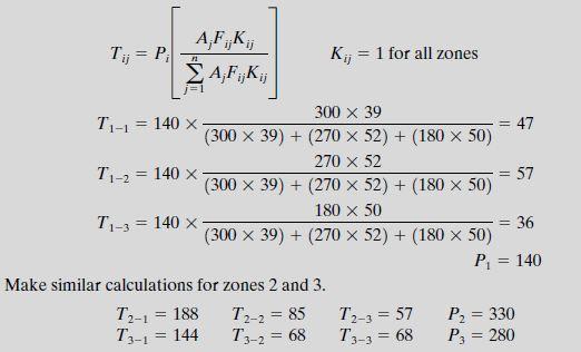
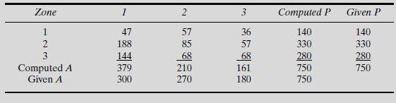
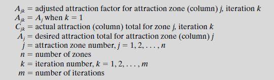
18 UTable:U Zone-to-Zone Trips: First Iteration, Singly Constrained.

19 UGrowth Factor Models Trip distribution can also be computed when the only data available are the origins and destinations between each zone for the current or base year and the trip generation values for each zone for the future year. This method was widely used when O-D data were available but the gravity model and calibrations for F factors had not yet become operational. Growth factor models are used primarily to distribute trips between zones in the study area and zones in cities external to the study area. Since they rely upon an existing O-D matrix, they cannot be used to forecast traffic between zones where no traffic currently exists. Further, the only measure of travel friction is the amount of current travel. Thus, the growth factor method cannot reflect changes in travel time between zones, as does the gravity model. The most popular growth factor model is the Fratar method, which is a mathematical formula that proportions future trip generation estimates to each zone as a function of the product of the current trips between the two zones Tij and the growth factor of the attracting zone Gj. Thus,

20 UExampleU Forecasting Trips Using the Fratar Model A study area consists of four zones (A, B, C, and D). An O-D survey indicates that the number of trips between each zone is as shown in Table below. Planning estimates for the area indicate that in five years the number of trips in each zone will increase by the growth factor shown in Table and that trip generation will be increased to the amounts shown in the last column of the table. Determine the number of trips between each zone for future conditions. UTableU Present Trips between Zones. UTableU: Present Trip Generation and Growth Factors.

21 UTable:U First Estimate of Trips between Zones. UTable:U Growth Factors for Second Iteration.

22

23

24

25

26

27