CIVL4332 L1 Introduction to Finite Element Method

Transcription

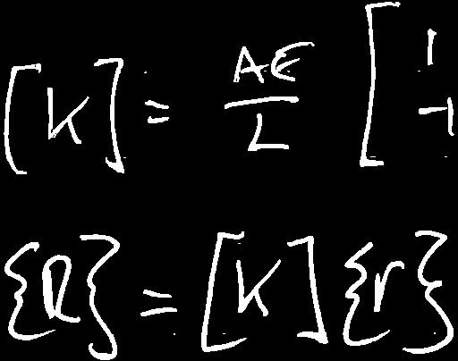
1 CIVL L Introduction to Finite Element Method CIVL L Introduction to Finite Element Method by Joe Gattas, Faris Albermani Introduction The FEM is a numerical technique for solving physical problems such as stress analysis. Using FE formulation, the equilibrium equation [] T [D]{}{u} + {B} = (.) is transformed into a system of simultaneous algebraic equations of the form [K]{r} = {R} (.) This transformation operates at the scale of individual domain subdivisions (finite elements), which are used as piecewise patches to build a complete D, D, or D domain. The stiffness method seen in CIVL similarly used an element discretization, with each element having an analytical stiffness and discontinuous nodal displacements. The FEM method has a numerical stiffness and a continuous displacement field. Advantages of FEM: versatility and accuracy control Disadvantages of FEM: numerical (rather than analytical) solution and large computer output. CIVL lectures on the finite element method are as follows. L: Introduction to Finite Element Method L: Continuum Mechanics: Stress and Equilibrium L: Continuum Mechanics: Strain and Constitutive Laws L: FEM: Formulation L5: FEM: Shape Functions L6: FEM: Isoparametric Elements page of 5

2 CIVL L Introduction to Finite Element Method FEM Analysis Types There are numerous types of finite element analysis. Different solutions can be obtained by using different forms of the general finite element stiffness equation: Linear Static Analysis: Kr = R. Non-Linear Static Analysis: [K + K G ]r = R, where K G is a geometric stiffness matrix that is a function of stresses. Linear Buckling (Eigenvalue) Analysis: K + cr K G =, where cr is the load factor for the critical buckling load. Does not solve deformation path but finds the point where displacement is possible without applied load (buckling). Dynamic Analysis: M r + Cṙ + Kr = R(t), where M is the mass matrix, C is the damping matrix, and ṙ and r first and second derivatives of displacement with respect to time. Natural Frequency (Vibration) Analysis: K+! M =, where! is natural frequency of the system. This lecture series shall primarily focus on linear static analysis. FEM Procedure Overview The broad procedure for the finite element method is as follows: Pre-processing. Select element type and discretization.. Displacement (shape) functions [N] are used to approximate the displacement field {u} within the element from using nodal values {r}, with {u} =[N]{r}.. Establish strain-displacement relations {"} =[]{u} and constitutive laws { } =[D]{"}.. The element stiffness relation is obtained, usually with an energy approach used to derive the stiffness [k e ]{r e } = {f e }. Solution 5. Assemble the structural stiffness matrix [K] and nodal force vector {R} from element stiffnesses [k e ] and element forces {f e }. 6. Impose boundary conditions and solve the global equation for nodal displacements [K]{r} = {R}. Post-processing 7. Stress recovery: element stresses are calculated by back-substitution into the element equation. page of 5

3 CIVL L Introduction to Finite Element Method Steps - are full finite element procedures that are simplified in the direct stiffness method seen in CIVL. The full FEM process is effective for elements of any complexity. Example.: Direct Stiffness vs Finite Element Formulate the element stiffness of a D truss element with area A, length L, and Young s modulus E using the Direct Stiffness and Finite Element methods. Direct Stiffness Method Truss elements have a single axial translational displacement and single corresponding axial force. Basic stiffness can be derived from basic linear elastic material elongation: " = /L = /E = P/(EA). [k] = AE L Δ P Transform basic stiffness to local x [k ]=T T kt = AE L 6 Sym. y system. D case: global x y axes align with local x y axes, consider x axis (u displacements) only. [k e ]= AE apple L 7 5 v i u i u j v j Finite Element Method Step : Displacement field and shape functions A truss element has two nodes, each with a nodal coordinate x, nodal displacement r, and nodal force f. It also has constant cross-section area A and length L. {u} = apple u u, {r} = apple r r, {f} = apple f f x A,L r, f x r, f page of 5

4 CIVL L Introduction to Finite Element Method A continuous linear displacement u field is assumed to exist between end nodes. Shape functions N are used to obtain intermediate displacement values from end node displacements r. u =[N]{r} =[ N N ] apple r r r u r = N r + N r Shape functions for a two-node element with a linear displacement field are: [N ]= [N ]= x L x L N N Step : Strain and stress fields The strain field for a D element is: ["] =" xx Strain is the differential of displacement: " xx =[/x]{u} =[/x][n]{r} =[B]{r} The stress field for a D element is: { } = { xx } Material constitutive laws relate stress and strain: { } =[D]{"} The B matrix is defined as the differential of N For D case, xx = E" xx so [D] =[E]. [B] =[][N] = [ /L /L] { xx } =[E]{"} =[E][B]{r} Step : Energy approach to obtain element stiffness Using an energy formulation if can be shown that element stiffness is equal to the integral of B T DB over the element volume. For a D element, volume V = AL, which gives: Z Z [k e ]= B T DBdV = A B T DBdx V L Z apple /L = A [E] [ /L /L] dx = AE apple /L L L Note: this integral is solved numerically, not analytically, in a typical FEM solver. page of 5

5 CIVL L Continuum Mechanics: Stress and Equilibrium CIVL L Continuum Mechanics: Stress and Equilibrium by Joe Gattas, Faris Albermani Continuum mechanics is an important part in the finite element method as stress and strain relationships are used to solve the stiffness integral. Coordinate system and Applied Forces Most problems are formulated in D in FEM so we shall adopt a D Cartesian right-handed coordinate system. This is referred to as the x i system, where i =,,. Axes x,x, and x are used instead of x, y, and z, respectively. x x x Within the a D Cartesian system we can locate a continuum, which is a continuous body. This continuum is general and can be broadly applied, for example as a fluid, magnetic field, traffic flow, etcetera. The present notes will focus on a structural type analysis for stresses of an elastic continuum. An elastic continuum can be subjected to some forces that induce stresses, strains, and displacements through the continuum. The forces at some point P within the body can be classified as: page 5 of 5

6 CIVL L Continuum Mechanics: Stress and Equilibrium Body force B i for i =,,. These are forces per unit volume or unit mass of the body. Example body forces include gravity loads and inertial forces. Surface traction Ti n for i =,,. These are forces per unit area (in D) or per unit length (in D). The traction is defined with reference to a plane with normal unit vector {n}. x B n T i n B B x x D Stress Definition The application of forces with induce a stress in the body. The stress at any point is defined with the Cauchy stress tensor [ ij]: [ ij] = 5 (.) For a D problem, the stress tensor has nine stress components at any point: Direct (Normal) Stress Components:,, Shear Stress Components:,,,,, It is essential to understand where these stresses are acting on the body and the sign convention used. A point P within a body can be enlarged to give the following infinitesimal volume dx dy dz. page 6 of 5

7 CIVL L Continuum Mechanics: Stress and Equilibrium x x P x x P x x Stress components ij act on the interfaces of this volume. The first index i denotes the interface and the second index j denotes the direction of the component, with positive directions corresponding to the outward normal vector of each face. Direct stresses are positive if both indices have direction vectors of the same sign, e.g. is positive if it acts on an interface with a normal in the direction of x and with a positive force in the direction of x. This gives tension as positive and compression as negative. Positive direct stresses are shown below. x Shear stresses are positive if both indices have direction vectors of the same sign, e.g. is positive if it acts on an interface with a normal in the direction of x and with a positive force in the direction of x. Positive shear stresses are shown below. x σ σ P σ x x σ σ σ P σ σ σ x x Example.: Stress Tensor Symmetry Prove that ij = ji for all i 6= j at any point in a continuum by using the three equations of moment equilibrium. page 7 of 5

8 CIVL L Continuum Mechanics: Stress and Equilibrium x σ σ σ σ σ O σ σ O σ σ σ σ σ x x σ x x Traction stress acts on an area dx dx. Traction stress acts on an area dx dx. Considering the sum of moments about axis x at point O: X Mx ==( dx dx )dx ( dx dx )dx dx dx dx = dx dx dx = Similar summations of M x and M x show = and =, respectively. The moment equations of equilibrium can thus be used to prove ij = ji. The stress tensor is therefore symmetric with six unique stress components, written as stress vector { } T = {,,,,, }. Stress Transformation A cut can be taken through point P to generate a plane with unit normal vector n. There will be stresses on the new interface, represented by traction vector {Ti n }. This stress vector can be obtained from the stress tensor as: {Ti n } =[ ij]{n} (.) The traction stress vector is composed of normal (direct) stress vector { n } and shear stress vector { }. The magnitude of the normal stress can be found be taking the dot product of {n} and {T n i }. The normal stress vector is then and { } can be found by subtraction of {T n i } and { n } n = {n} T {T n i } (.5) { n } = n {n} (.6) { } = {T n i } { n } (.7) page 8 of 5

9 CIVL L Continuum Mechanics: Stress and Equilibrium D Case x D Case x n σ n τ n σ n τ T i n x x T i n x Example.: Octahedral Traction Stress The octahedral plane is the plane whose normal vector makes equal angles with coordinate system axes, that is with equal direction cosines of / p. Calculate the normal (direct) and shear stress components on the octahedral plane through point P given it has the following stress tensor: ij = MPa x The octahedral plane has the following normal vector: {n} = n n n 5 = / p / p / p 5 n The traction vector is given as: The normal component is: {T n i } =[ ij]{n} x x =[., 8.7,.] T MPa { n } = {n} T {T n i }{n} =[.7,.7,.7] T MPa page 9 of 5

10 CIVL L Continuum Mechanics: Stress and Equilibrium The shear stress component is: { } = {T n i } { n } =[.7,.,.] T MPa In addition to finding stress on target plane, a complete [ ij] defined in a new coordinate system u i can be obtained with rotation of stress tensor[ ij] defined in old coordinate system x i. Old and new stress tensors are related by: [ ij] =[L][ ij][l] T (.8) where [L] is a rotation matrix containing direction cosines a between old and new system axes. a u x a u x a u x [L] = a u x a u x a u x 5 (.9) a u x a u x a u x x u - cos a u u x x x u u - cos a u x - cos au x Stress Invariants, Principal Stresses, and Stress Decomposition A stress tensor will change depending on a chosen coordinate system orientation, however it possesses three stress invariants that are constant across all orientations. As stress invariants are the same in any orientation, they can be used to check stress transformations, i.e. I = I, I = I, and I = I, where I, I, and I are the first, second, and third stress invariants, respectively. The first stress invariant is the sum of direct stresses: I = + + (.) The second stress invariant is the sum of the three minors of the stress tensor: apple apple apple I = + + (.) page of 5

11 CIVL L Continuum Mechanics: Stress and Equilibrium The third stress tensor is the determinant of the stress tensor: I = ij (.) If a cut is made on an appropriate plane through a point in a continuum, the traction stress vector will correspond to the normal stress vector, i.e. shear stress on that plane is zero. This corresponds to the principal stress state. It is the D version of the D principal stresses seen in CIVL. x n n T i = σn σ σ σ σ τ τ x τ τ n Mathematically this is represented as: [ ij]{n} = {n} (.) The solution to this equation in terms of unknown is given as: ( ) ( ) 5 {n} = (.) ( ) A non-trivial solution to this equation occurs when Det ij =, which is a cubic polynomial in terms of. The three cubic roots,, are the three principal stresses at that point, such that > >. The characteristic cubic equation for principal stresses can be written as I + I I = (.5) Three principal stress directions are {n }, {n }, and {n } associated with principal stress directions,, and, respectively. They can be found by back-substitution of the principal stresses into (.). For a principal stress state, the stress invariants simplify to: I = + + (.6) I = + + (.7) I = (.8) page of 5

12 CIVL L Continuum Mechanics: Stress and Equilibrium Any stress state [ ij] can be decomposed into the deviatoric stress tensor [s ij ] and the hydrostatic pressure p: [ ij] =[s ij ]+p[ ij ] (.9) where p = I / and [ ij ]=if i = j but otherwise is zero, i.e. it is a identity matrix. Deviatoric stress is thus given by: ( p) [s ij ]=[ ij] p[ ij ]= ( p) 5 (.) ( p) These two values represent important phyical aspects of the point under consideration. The deviatoric stress corresponds to deformation. It represents a pure shear stress state which has n =, 6=, and I =and is usually responsible for failure of the material; it is used to derive the von-mises yield criterion discussed below. The hydrostatic stress is responsible for dilation. Hydrostatic Deviatoric There are six stress components in a general stress state or three stress components in a principal stress state. When assessing material failure is is convenient to express the stress as a single value. For ductile materials such as metals, the von-mises (effective) stress is most appropriate and is given by: VM = r ( ) +( ) +( ) +6( + + ) (.) For a principal stress state this simplifies to: VM = r ( ) +( ) +( ) (.) von-mises stress is always positive so cannot be used to indicate load direction and it can be higher than the maximum principal stress. Different effective failure stress relationships should be used for other materials, for example the Drucker-Prager yield criterion can be used for concrete. The principal shear stresses can be obtained from principal direct stresses from Mohr s circle manipulations as: = / (.) = / (.) = / (.5) page of 5

13 CIVL L Continuum Mechanics: Stress and Equilibrium Equilibrium Equations The three moment equilibrium equations were used to generate a symmetric stress tensor. Three force equilibrium equations remain. Consider forces acting on an infinitesimal element in the x direction: σ + σ x x σ σ + σ dx B x x dx x σ dx σ σ x x x x σ + σ x x In addition to the traction forces acting on element interfaces there is a body force B. F x == which reduces to x x x + x x x + x x x +B x x x (.6) x x x x + x + x + B = (.7) This can be repeated for directions x and x, which can be written in shorthand as: where ji,j is the differential of ji with respect to j. ji,j + B i = (.8) In matrix form this becomes: where [] T { } + {B} = (.9) [B] T = {B,B,B } (.) [ ] T = {,,,,, } (.) x x [] T = x x x x The differential operator [] T is extensively used in FEM. x x x 5 (.) page of 5

14 CIVL L Continuum Mechanics: Stress and Equilibrium Example.: Principal Stresses Calculate the principal stresses and associated principal stress directions, given that: 9 5 ij = 5 MPa Sym. 8 and one of the principal stresses is MPa. The invariants of the given stress tensor are: I = + + = apple apple I = + apple + I = ij = = 68 = 8 5 = 86 Given a principal stress of MPa, ( ) is a factor of the characteristic equation I +I I =: I + I I == ( )(a + b + c) =a +(b a) +(c b) c which gives a =, b =6, and c = 6. The roots of (a + b + c) are.8mpa and -6.8MPa, which gives principal stresses as: =.8 MPa, =MPa, = 6.8 MPa Substitution of a principal stress into the princpal stress solution gives: ( ) 9 5 n x ( ) 5 n 5 x = Sym. (8 ) n x 5 (.) This equation cannot be solved directly as it has already been used to generate the principal stresses. Use the additional condition that {n } T {n } =: n x n x n x n x ( ) 5 n 5 x = 5 (.) Sym. (8 ) n x which gives {n } T = ±{.6,.,.87}. A similar substitution gives {n } T = ±{.6,.85,.5} and {n } T = ±{.859,.8,.78}. page of 5

15 CIVL L Continuum Mechanics: Strain and Constitutive Laws CIVL L Continuum Mechanics: Strain and Constitutive Laws by Joe Gattas, Faris Albermani Analysis of Strain The strain tensor [" ij ] is similar to the stress tensor, i.e. it defines the strain field at a point in a continuum: " " " [" ij ]= " " " 5 (.5) " " " The tensor is symmetric, " ij = " ji, and so has six unique strain components, written as stress vector {"} T = {",",",,, }. The first three components are direct strains and the second three components are the engineering shear strain components where ij =" ij, discussed further below. Direct strain components represent the length change between two points in a continuum, with positive taken as extension and negative as contraction. Finite-element uses Green-Lagrange strain, defined as: " = (L o + L) L o = L + L L o L o L o L for small strain ( < %) (.6) L o where L o is the initial length between two points and L o + L is the length of the same two points after deformation. If L =after load is applied to a body than there has been a displacement without change in length and the body has undergone a rigid body motion. This small displacement strain " = L/L o is called engineer s strain and is as previously used in structural mechanics courses. For large displacements, logarithmic or true strain e is used instead of ": e = Z L L o dl L =lndl L (.7) page 5 of 5

16 CIVL L Continuum Mechanics: Strain and Constitutive Laws Shear strain components represent the change in angle between three points in a continuum: = o (.8) where o is the initial angle between three points and is the angle of the same three points after deformation. Direct Strain Shear Strain B L o A B A L o +Δ L B C θ o A B A C θ For all strain components, the first subscript denotes the direction of the fibre under strain and the second subscript denotes the direction of the fibre s displacement. All transformations derived for the stress tensor are also valid for the strain tensor, e.g. a traction vector for strain on an interface with unit normal vector n is n =["]{n}. How the strains are occurring within the body and can be understood as follows. For direct strains, consider a D fibre with initial length dx. dx dx + u x dx x For shear strains, consider two fibres with side lengths dx and dx : x u x dx ε γ ε u dx After load is applied, it has length: dx + u x dx The engineer s strain is then: " = L L o = u x (.9) After load is applied, these are distorted to generate two angles. Using a small angle trigonometric approximation (tan x = x), there are: " = u x, " = u x (.) ", ", and " are referred to as tensorial shear strains as they correspond to strain tensor components. It is more common to the alternate definition referred to as engineering shear strains where all shear displacement acts on a single edge: ij =" ij. page 6 of 5

17 CIVL L Continuum Mechanics: Strain and Constitutive Laws Example.: Strain Transformations The is a interface cut ABC within a continuum. Point A, B, and C are located a unit distance along axes x, x, and x respectively. Point D is located halfway between points A and B. During an experiment, the strain ["] is measured at D as: ["] =..5.. Sym.. 5 (.) Calculate the change in the right angle ADC. x B D A C x x The points have the following coordinates: A =[,, ] B =[,, ] C =[,, ] D =[.5,.5, ] The change in angle is a shear strain. Material direction of two fibres! DA = A D =[.5,.5, ]! DC = C D =[.5,.5, ] page 7 of 5

18 CIVL L Continuum Mechanics: Strain and Constitutive Laws Convert these to a unit vector: n DA = n DC =! DA DA! DC DA = [.5,.5, ] / p = p 8 < : = [.5,.5, ] p / p = p 6 8 < : 9 = ; 9 = ; We can check if unit vectors are correct as they are orthogonal n T DA n DC =. Strain vector of fibre DC n 8 { DC} n =["]{n DC } = p < 6 : = ; (.) DC can be projected onto {n DC} to find the direct strain component. As {n DC } and {n DA } are orthogonal, n DC can be projected onto {n DA} to find the shear strain component. The change in angle ADC is ADC =" ADC =.58 rad. " ADC = {n DA } T { n DC} =.9 rad. (.) x δ n DC ε ADC x x page 8 of 5

19 CIVL L Continuum Mechanics: Strain and Constitutive Laws Strain-Displacement Relations At any point P in a continuum, there are three displacements u i, where i =,,. Strain is the partial derivative of displacement and so given the displacement vector {u} T = {u u u }, strain-displacement relations can be written as: 6 " " " {"} =[]{u} (.) u x x x u x u u x = u x x 5 x = u 7 u 6 x + u (.5) x u x x x x x + u x u x + u x where [] is defined for stress equilibrium relations and engineering shear strains are given in the strain vector, not tensorial shear strains. This relation shows that three displacements generate six components of strain. Going in the opposite direction however, six strain components cannot determine a unique continuous displacement field, as the system is overdeteriminant. The strain components therefore have to be constrained by compatibility equations. Six compatibility equations similar to the one below need to be satisfied in a D system. " x + " x " x x = (.6) Of the six D compatibility equations, three are independent. All but the first equation shown above is automatically constrained in a plane strain or plane stress field. The compatibility equations are generated as follows. Shear strain is related to displacement with: u = + u =" x x Deformation u must be continuous and there must be some gradient in the strain field, i.e. " /x 6= and " /x 6=. The strain gradient can therefore be obtained by taking the derivative of the previous equation: u + u = " x x x x x x Direct strain relations " = u x and " = u y can be substituted to simplify: " x which gives the compatibility equation (.6). + " x = " x x page 9 of 5

20 CIVL L Continuum Mechanics: Strain and Constitutive Laws Constitutive Laws Thus far, we have related forces to stress and displacements to strain. The final relations required are those to link stress and strain. The relations are termed constitutive laws and are to do with the system material. It is therefore more complicated that prior relations which only relate to system geomety. The general form of the constitutive law is written the matrix [D] that relates stress and strain as follows. { } =[D]{"} (.7) The simplest material is an isotropic, linear elastic material. The linear elastic material requires only two material properties to define: Young s Modulus E and Poisson s ratio v which are obtained from material tests. The isotropic linear elastic material is the simplest case of the constitutive law. Orthotropic materials such as composite laminates require 9 material properties to define, and completely anisotropic materials require material properties to define. For direct stresses in an isotropic material, there is coupling from the Poisson s effect. An axial stress will induce an axial strain of E" and transverse strains of " = v" and " = v". σ ε = -vε σ σ E σ G ε ε γ For shear stresses in an isotropic material there is no coupling. A shear stress of G, where G is the shear modulus related as: G = E ( + v) will induce an axial strain (.8) This gives the following stress-strain relation: 6 " " " = 7 E 6 5 v v v ( + v) ( + v) Sym. ( + v) (.9) page of 5

21 CIVL L Continuum Mechanics: Strain and Constitutive Laws the inverse of this gives the constitutive matrix as: [D] = E ( + v)( v) 6 v v v v v v v Sym. v v 7 5 (.5) All natural materials have <v<.5. As v!.5 the material becomes incompressible as the /( v) causes [D]!. Meta-materials are those that have been engineered to possess properties not found in nature, including negative Poisson s ratios, i.e. <v<. There are termed auxetic materials and include origami-inspired meta-materials, applied for example as a deployable stent : Recalling the equilibrium relation of this previous lecture. This can now be written with the constitutive law and using the strain-displacement relation as: [] T { } + {B} = [] T [D]{"} + {B} = [] T [D]{}{u} + {B} = (.5) Figure taken from You, Z. and Kaori K. Expandable tubes with negative Poissons ratio and their application in medicine. Origami: Fourth International Meeting of Origami Science, Mathematics, and Education. 9. page of 5

22 CIVL L Continuum Mechanics: Strain and Constitutive Laws Continuum Mechanics Summary The relations in D continuum mechanics can be summarised as follows. Forces B i, T n i Stiffness [] T [D]{}{u} + {B} = Displacements {u i } Equilibrium Equations [] T { } + {B} = Strain-Displacement Relations 6 {"} = []{u} Stress components 6 { } Constitutive Laws 6 { } = [D]{"} Strain components 6 {"} There are 5 unknown quantities: 6 stress components, 6 strain components, and displacement components. These are found with 5 relations: equations of equilibrium, 6 strain-displacement relations, 6 constitutive laws. The stiffness relation can be used to solve displacements directly, but element stresses and strains must then be calculated back-substitution into other relations. Simplified (D and D) Mechanics The above derivations are for complete D continuum systems. All lower-order structural systems can be obtained from simplified continuum conditions as follows. D Truss Element with x longitudinal axis and u longitudinal displacements only. {u} = u {"} = " = u /x [] =/x { } = = E" [D] =E F x x,u page of 5

23 CIVL L Continuum Mechanics: Strain and Constitutive Laws D Beam Element with x longitudinal axis, x transverse axis, and u and u displacements only. {u} = u = x u x {"} = " = u /x = x u /x [] = x /x { } = = E" [D] =E x,u Fx F x x,u θ = du / dx D Plane Stress A D continuum located in the x x plane with all stresses in-plane and an out-of-plane length much smaller than in-plane lengths x << x and x << x, for example as in a cantilever with an end point load. Two in-plane displacement components: {u} T = {u u } All stress is in plane, i.e. there is no out-of-plane stress = = =, leaving three stress components: { } = { } There is no coupling in shear strain so = =. There is coupling for direct strain so there will be out-of-plane (Poisson) expansion or contraction " 6=: {"} T = {" " } " = v(" + " ) F x,u O Fx x,u σ x σ σ O σ x σ σ Stress-displacement relations and constitutive laws are then: [] = x x x x 5 and [D] = E v v v v 5 (.5) page of 5

24 CIVL L Continuum Mechanics: Strain and Constitutive Laws D Plane Strain A D continuum located in the x x plane with all strains in-plane and an out-of-plane length much larger than in-plane lengths x >> x and x >> x, for example as in a dam with uniform hydrostatic pressure along length. Two in-plane displacement components: {u} T = {u u } All strain is in plane, i.e. there is no out-of-plane strain " = " = " =, leaving three strain components: {"} T = {" " } There is no coupling in shear stress so = =. There is coupling for direct stress so there will be out-of-plane stress 6=: x,u O x,u ε ε O ε x ε { } T = { } = v( + ) Stress-displacement relations and constitutive laws are then: [] = x x x x 5 and [D] = E ( + v)( v) ε v v v v v ε 5 (.5) D Thin Plate Element A D element with x longitudinal axis, x transverse axis, and u, u, and u displacement components. The element has out-of-plane stress and strain, but is assumed to be thin x << x and x << x such that out-of-plane shear can be neglected = =. {u} = u = x u {"} T = {" " } apple [] T = x x x x { } T = { } x x u and constitutive matrix [D] the same as for the plane stress case. x,u θ = d / dx u x,u Fx θ = x,u d / dx u page of 5

25 CIVL L Continuum Mechanics: Strain and Constitutive Laws Example.: D Continuum Mechanics Establish an equivalent D system for the following D bodies: a) A long, thick-walled cylinder under constant internal pressure. b) A fin web connection plate. a) The cylinder has no longitudinal stress, so a plane strain condition can be assumed. σ r σ θ b) The fin plate has no out-of-plane stress, so a plane stress condition can be assumed: σ σ page 5 of 5

26 CIVL L FEM Formulation CIVL L FEM Formulation by Joe Gattas, Faris Albermani As stated in earlier lectures, the Finite Element Method transforms the continuum mechanics equilibrium equation [] T [D]{}{u} + {B} =into a system of numerically-solvable simultaneous algebraic equations of the form [K]{r} = {R}. The following lecture describes the necessary steps to achieve this transformation and thus generate a complete FEM formulation. Discretization The first step in the Finite Element Method is to break up the continuum to be solved into discrete elements in a process that is called discretization. The need for a discretized form arises because the equilibrium equation is written in terms of an unknown displacement field {u}. For a general continuum, it is difficult to know the form of this displacement field. However it is easy know the displacement field for a small element, for example a -node bar element or -node square element. The continuous displacement field for the whole continuum is therefore easier to approximate as a stepwise assembly of small elements. It is essential to choose an element suitable for the particular problem, e.g. a disc cannot be approximated with D truss elements, but could be approximated with D plate elements. The process is analogous to curve-fitting with a straight-line approximation, i.e. it is difficult to determine a function to fit a complex curve, but it is easy to assume a straight line between discrete points on the curve to generate approximately the same form. page 6 of 5

27 CIVL L FEM Formulation Exact Coarse Appx. Fine Appx. As with any approximation, there is some error between the approximate and ideal system. The necessary level of discretization varies substantially between FEM models. It is therefore always necessary to undertake a mesh refinement or mesh sensitivity study. Such studies increase the number of elements (e.g. from 8 to 6 to elements) or the change element type (e.g. quad or tri plate elements) systematically to establish a mesh type and density that gives a stable solution. Displacement (Shape) Functions Shape functions are used to transform nodal displacements {r} into a continuous displacement field {u}. {u} =[N]{r} (.5) where [N] is the shape function matrix. This consists of individual shape functions N to relate each nodal displacement to the continuous displacement in a particular element: 8 >< {u} =[N N N N ] >: r r r r 9 >= >; {u} = N r + N r + N r + N r x r r u r x x r page 7 of 5

28 CIVL L FEM Formulation The above relation allows stress and strain fields to be expressed directly in terms of nodal displacements: where [B] is the shape function derivative matrix: {"} =[]{u} =[][N]{r} =[B]{r} (.55) { } =[D]{"} =[D][B]{r} (.56) The next lecture wll discuss how to generate suitable shape functions. Energy Formulation for Element Stiffness [B] =[][N] (.57) Previously, stiffness has been derived for elements directly as the inverse of flexibility coefficients obtained from structural mechanics solutions. This is feasible for simple elements such as D truss, beam, or frame elements, however for more complex elements it is challenging, e.g. an 8 or -node brick element. Instead, an energy approach is used in FEM to calculate the element stiffness matrix as follows. Internal (Strain) Energy The internal (strain) energy U of a system is found by integrating the stress times strain over the volume V of material in the body: U = Z { } T {"}dv (.58) This can be expanded in terms of stress and strain components. D case with uniform cross-section: Z V U = A " dx D case with uniform thickness: Z Z U = t " + " + " dx dx Full D case: Z Z Z U = " + " + " + " + " + " dx dx dx Internal energy (.58) can also be expressed in terms of nodal displacements by substituting (.55) and (.56). This gives: U = Z { } T {"}dv V = Z ([D][B]{r}) T ([B]{r})dV V = Z {r}t [B] T [D][B]dV {r} (.59) page 8 of 5

29 CIVL L FEM Formulation External Energy The external energy is generated as the sum of work W S from traction forces {T }, W B from body forces {B}, and W N from nodal forces {f n } applied to the body: W = W S + W B + W N Z Z = {u} T {T }ds + {u} T {B}dV + {r} T {f N } (.6) where S is the surface over which the traction force {T } is applied. W S and W B can also be written directly in terms of nodal displacement vector. From (.5), it is known that {u} T = {r} T [N] T. This gives: Z Z W S = {u} T {T }ds = {r} T [N] T {T }ds = {r} T {f S } (.6) Z Z W B = {u} T {B}dV = {r} T [N] T {B}dV = {r} T {f B } (.6) W = {r} T ({f B } + {f S } + {f N }) (.6) = {r} T {R} (.6) where {f S }, {f B }, and {R} are energy-equivalent nodal load vector for surface, body, and all loads, respectively. Energy Equilibrium Of all displacements that might satisfy the boundary conditions of a structure, those that satisfy the equations of equilibrium occur when there is a stationary value of potential energy, i.e. the difference between internal work and external work is at a minimum. Π Unstable Equilibrium Neutral Equilibrium u Stable Equilibrium The total potential energy is related to internal work U and external work W as: =U W (.65) The stationary condition is then = U W = (.66) where is a small admissible variation. In other words, when a structure is subjected to a load, it will find a deformed configuration that uses the minimum amount of energy to achieve a certain displacement. page 9 of 5

30 CIVL L FEM Formulation Equilibrium therefore is given by: {r} = U {r} U {r} = W {r} W {r} = Substituting (.58) and (.6) then gives: ( R {r}t [B] T [D][B]dV {r}) {r} Z [B] T [D][B]dV = ({r}t {R}) {r} {r} = {R} [K]{r} = {R} where stiffness matrix [K] is: Z [K] = [B] T [D][B]dV (.67) Example.: Spring Element Use the energy approach to derive the stiffness matrix of D spring element: k e r e = f e k r, f r, f A two-node spring element has nodal displacements {r} T = {r r } and nodal forces {f} T = {f f }. Internal energy is: Z Z U = { } T {"}dv = A V Z Z L " dx r r dx External work is: = AE = AE L " dx = AE (r r ) = k (r r ) W = r f + r f L page of 5

31 CIVL L FEM Formulation Potential energy is: which is stationary when: The non-trivial solutions to this are when r =U W = k (r r ) == r r + r r =and r =: r f r f =gives k(r r r )=f =gives k(r r r )=f which is matrix form becomes apple k apple apple r f = r f FEM Formulation Summary The FEM formulation is therefore primarily concerned with expressing the main unknowns in a system stiffness equation in terms of nodal displacements. It can be summarised as follows: Displacement Field {u} =[N]{r} Strain Field {"} =[]{u} =[][N]{r} =[B]{r} Stress Field { } =[D]{"} =[D][B]{r} Element Strain Energy U = Z { } T {"}dv = Z {r}t [B] T [D][B]dV {r} External Energy W = W N + W B + W S = {r} T {R} Stationary Potential = U W =, which gives Z Stiffness Relation {R} =[K]{r} = [B] T [D][B]dV Z Stiffness Matrix [K] = [B] T [D][B]dV {r} Example.: FEM Truss Stiffness Revisit the Finite Element formulation of a D truss element shown in Example.. page of 5

32 CIVL L5 FEM Shape Functions CIVL L5 FEM Shape Functions by Joe Gattas, Faris Albermani Displacement Fields Consider the following element with an axial load, length L, cross-section area A, and Young s Modulus E. In a finite element formulation it can be discretise into five D elements, each with length l. L,A,E 5 l A general form of the displacement field for axial (D) loading is as a polynomial function over the beam length with degree n : u(x) =a + a x + a x a n x n (5.68) which has n coefficients and apple x apple L. Coefficient a does not contribute to the strain field and so it corresponds to rigid body motion. The remaining coefficients correspond to displacement gradients. The degree of polynomial necessary to approximate the field depends on the complexity of the problem. An element with a uniform axial load has a uniform stress and strain. Strain is the derivative of displacement, so a uniform strain gives a linear displacement field, i.e. a first-degree polynomial. An element with a non-uniform axial load will have a non-uniform strain and so a higher-order polynomial is necessary for approximation. The number of derivatives of displacement that are continuous between elements is referred to as the degree of continuity of an element. A C element has zero continuous derivatives i.e. it is continuous in page of 5

33 CIVL L5 FEM Shape Functions terms of displacement only. A C element has a continuous first derivative of displacement (strain) as well as continuous displacement. C u C C u u ε ε ε Displacement Fields with Shape Functions The D element in the previous section with a uniform axial load has a linear displacement field. This can be expressed as: u = a + a x {u} =< x> where {a} is the vector of polynomial coefficients. a a {u} =< x>{a} (5.69) Nodal displacements values u(x =)=r and u(x = l) =r can be used to relate polynomial coefficients to nodal displacements. In matrix form this becomes: apple r a = r l a {r} =[A]{a} (5.7) {a} =[A] {r} (5.7) where [A] = apple l (5.7) l Substituting (5.7) into (5.69) give: {u} =< x>[a] {r} {u} =[N]{r} (5.7) where [N] is a matrix containing the shape or interpolation functions: [N] =<x>[a] (5.7) page of 5

34 CIVL L5 FEM Shape Functions which for this example is: [N] =< =< N = N = x l x> l x l x l apple l x l > (5.75) (5.76) This is expressed in the physical coordinate system however it can also be expressed in the natural coordinate system by replacing the normalised x/l term with : where apple apple. N = N = All shape functions have some common properties: they are always between and ; they have a value of at their own node and at every other node; the sum of shape functions is equal to at any point in the element; and the superposition of shape functions times nodal displacements gives the whole displacement field. N + N N N r u r N r N r N r + N r Lagrange Interpolation The above uses a polynomial function to generate shape functions. Another approach is to use Lagrange interpolation to generate shape functions directly. Lagrange interpolation represents a field for an element with a polynomial field of degree p is represented as: nx = L xi i (5.77) page of 5

35 CIVL L5 FEM Shape Functions where L xi is the Lagrange function, is some field (displacement, stress, strain, etc.), i is the field value at node i, and the number of nodes n is one greater than the polynomial degree, i.e. n = p +. For a Lagrange displacement field = u, i = r i, and so L xi = N i. nx = L xi i = L x + L x L xn n+ u = N r + N r N n r n As Lagrange interpolation is for displacement only, Lagrange elements are C elements. The Lagrange function is a chain product ( ) along all element axes: L xi = n j+(x j x) n j+ (x, for i 6= j (5.78) j x i ) Example 5.: Lagrange Shape Functions Use Lagrange interpolation to find shape functions for a D element: i) with a linear (first-order) displacement field. ii) with a quadratic (second-order) displacement field. Plot the quadratic shape functions. i) A D linear displacement field requires p +=nodes. L x = N = (x x) (x x ) L x = N = (x x) (x x ) = (l x) l = ( x) l = = x l x l x l x ii) A D quadratic displacement field requires p +=nodes, with coordinates x =, x =.5l, x = l. L x = N = (x x)(x x) x (x x )(x x ) = x l + l L x = N = (x x)(x x) x (x x )(x x ) =x l l L x = N = (x x)(x x) (x x )(x x ) = x x l + l x x x page 5 of 5

36 CIVL L5 FEM Shape Functions Quadratic shape functions are: N N N D Shape functions Tri Element A triangular element has nodes, each with two displacements (r x, r y ) per node. r 6 r 5 r y r r x r The element has a displacement field that can be represented as a two-variable polynomial: u = a + a x + a y + a x + a 5 xy + a 6 y +... (5.79) A bilinear triangular has a linear displacement field in both x and y direction: u = a + a x + a y {u} =< x>{a} 8 < {u} =< x y > : a a a 9 = ; (5.8) Considering first x-displacements, nodal coordinates (x,y ), (x,y ), and (x,y ) are used to relate polypage 6 of 5

37 CIVL L5 FEM Shape Functions nomial coefficients to nodal displacements: 8 < : {r} =[A]{a} (5.8) = x y < a = ; = x y 5 a (5.8) : ; x y a r r r 5 The displacement field {u} in the x directions is then: {u} =< x>[a] {r} =[N]{r} 8 < =[N N N ] : r r r 5 9 = ; (5.8) N N N r r 5 r u N + N + N N r + N r + N r 5 The displacement field {v} in the y directions is also linear, so can be represented by the same displacement functions: 8 9 < r = {v} =[N N N ] r (5.8) : ; r 6 and a complete displacement field description is then: {u} = u v apple N N = N N N N 8 >< >: r r r r r 5 r 6 9 >= >; (5.85) page 7 of 5

38 CIVL L5 FEM Shape Functions Each shape function is associated with a single element node and shares the same properties as the D example shape functions, i.e. N + N + N =, etc. The general form of the shape functions for a triangle C element with a linear displacement field is: N i = xb i + yc i + f i P f i = xb i + yc i + f i A (5.86) where: b i = y j y k (5.87) c i = x k x j (5.88) f i = x j y k x k y j (5.89) where if i =, j =and k =; if i =, j =and k =; and if i =, j =and k =. Example 5.: Tri Element Displacement Field A three-node constant strain triangular finite element has nodal coordinates (x, y) of (,), (6,), and (,8) and nodal displacements (u, v) of (,), (-,), and (-,-). For a plane stress case, calculate the element: i) shape functions; and ii) stress components, assuming the element has a Young s Modulus of MPa and a Poisson s ratio of.. i) A constant strain element has a linear displacement field, so Lagrange interpolation can be used to find shape functions: b = y y = c = x x = f = x y x y =6 b = y y =6 c = x x = f = x y x y = b = y y = c = x x = f = x y x y = A = f + f + f = Shape functions are then as per (5.86) N = N = N = x + y +6 6x + y x +y + page 8 of 5

39 CIVL L5 FEM Shape Functions ii) The shape function derivative matrix is given as: [B i ]=[][N i ]= x y y x 5 apple N = N A b i c i c i b i 5 Stress and strain can be generated from shape function derivatives: { } =[D]{"} =[D][B]{r} = E v =. 8 < = : v v v... 9 = ; MPa 8 >< 5 [B B B ] 5 >: u v u v u v 9 >= >; >< 5 >: 9 >= >; Quad Element A bilinear quadrilateral plate element has linear displacement field in both directions. A linear first-order polynomial in requires n = p +=nodes, per direction, so the quad element requires (p +) = nodes. Nodes should be numbered to either anti-clockwise or clockwise. Either is suitable as long as it is consistent across elements. If expressed in the physical (x, y) system, the quad plate has width a and height b. In FEM formulations it is easier to work in the natural (, ) system, where x = a, and y = b. The Lagrange chain product generates C element shape functions when multiplied along all coordinate page 9 of 5

40 CIVL L5 FEM Shape Functions axes: N i = L L N = = N = = N = = N = = ( )( ) ( + )( ) ( + )( + ) ( )( + ) The general form of this is: N i = ( + i)( + i ) (5.9) v u y b x v u (-,) η ξ (,) v u a v u (-,-) (,-) Higher Continuity and Hermite Interpolation Increasing the degree of polynomial for a particular element will increase the complexity of the displacement field, however it will not increase the continuity of the field between elements. For example, a beam element has a cubic displacement field so has n = p + = nodes per element. A series of cubic C beam elements will have continuous displacement v but not a continuous displacement gradient. 8 >< {u} =< x x x > >: a a a a 9 >= >; (5.9) page of 5

41 CIVL L5 FEM Shape Functions Lagrange interpolation always produces a C element so a different interpolation is used for higher-continuity: the Hermite interpolation. It uses the same polynomial but increases the DOF per node instead of the number of nodes per element. A Hermite C beam element will therefore interpolate both deflection v and deflection gradient. C θ = dv/ dx C θ v v v v v v Deflection v and rotation can be written as polynomials as: v = a + a x + a x + a x = v x = a +a x +a x Four boundary conditions are then found with substitution of nodal values: v i θi θ j v j v(x =)=v = a v(x = l) =v = a + a l + a l + a l (x =)= = a (x = l) = = a +a l +a l The polynomial coefficient matrix is therefore a matrix: 8 >< >: {r} =[A]{a} 9 >= v v = >; 6 l l l l l 8 >< 7 5 >: Shape functions can then be obtained from [N] =<x>[a] as a a a a 9 >= >; (5.9) N = + for v (5.9) N = L( ) for (5.9) N = for v (5.95) N = L( ) for (5.96) page of 5

42 CIVL L5 FEM Shape Functions N N N N page of 5

43 CIVL L6 FEM Isoparametric Elements CIVL L6 FEM Isoparametric Elements by Joe Gattas, Faris Albermani Introduction Development of finite elements in terms of global coordinate system is only possible for simple types of elements. For more versatile elements (e.g. non-rectangular elements, elements with curved sides, elements a different orientations in space, etc.) isoparametric formulation is used Isoparametric elements are elements for which the same shape functions are used to interpolate element displacement field as well as element geometry. The element can then be formulated in natural coordinate system defined by the element geometry rather than its orientation in the physical coordinates system. Mapping between the natural and physical systems is used in the element formulation as: Displacement field: {u} =[N]{r} Element geometry : {X} =[N]{C} Where {r} and {C} are element nodal displacement and element nodal coordinates, respectively. For isoparametric elements [N] and [N] are identical. If [N] is of a higher degree than [N] the element is subparametric (the reverse is superparametric). page of 5

44 CIVL L6 FEM Isoparametric Elements Example 6.: Isoparametric Geometry A three-node triangular finite element has the following interpolation for element geometry and displacement field: nx = Nodal coordinates (x, y) are (,), (8,), and (,6) and corresponding nodal horizontal displacements are, -, and mm. Calculate the horizonal displacement within the element at location (,). L xi i Lagrange interpolation is used for element geometry and displacement field. The element therefore has a linear interpolation and shape functions can be evaluated from polynomial u = a + a x + a y as seen in previous examples. However, as displacement is only required at point P =(, ), an alternate method can be used to only evaluate shape function values at point P: u P = N,P u + N,P u + N,P u As it is an isoparametric element, geometry can be used to solve these shape function values: One additional equation is obtained from P N i =: Solving this system of equations gives: Substitution gives horizonal displacement as: x P = N,P x + N,P x + N,P x = y P = N,P y + N,P y + N,P y = N,P + N,P + N,P = N,P =, N,P = 6, N,P = 6 u P = 6 6 = Lagrange interpolation is used to map the physical coordinates (x, y) of an irregular element to a regular template element expressed in natural coordinates (, ). The coordinate from any point P within the template element can be mapped to the physical element using the same shape functions obtained for displacement field mapping, multiplied by the nodal coordinates rather than nodal displacements. page of 5

45 CIVL L6 FEM Isoparametric Elements x y (, ) P( x, y) x y (, ) (-,) P(ξ,η) (,) x y (, ) y,v x,u x y (, ) (-,-) (,-) η ξ Interpolation of displacement field: {u} = u v apple N N =[N]{r} = N N N N N N 8 >< >: u v u v u v u v 9 >= >; Interpolation of element geometry: {X} = x y apple N N =[N]{C} = N N N N N N 8 >< >: x y x y x y x y 9 >= >; (6.97) where the shape function is as described in the previous lecture for a bilinear quad element: N i = ( + )( + i ) page 5 of 5

46 CIVL L6 FEM Isoparametric Elements Jacobian Matrix The shape functions N i are written in the natural system (, ), however the strain matrix [B i ]=[][N i ] requires differentiation with respect to the physical system (x, y). The Jacobian matrix is therefore used to map differentials w.r.t. the natural system to differentials w.r.t. the physical system: =[J] x y (6.98) where the Jacobian [J], is: [J] = " x x y y # (6.99) Computationally, this is evaluated as: [J] = " N N N N N N N N # 6 6 x y x y x y x y 7 5 (6.) After calculation of [J], the inverse is found as: x y =[J] apple j j = j j = j + j j + j (6.) where j,j,j,j are elements of the Jacobian inverse. The shape function derivative matrix can then be expressed in natural coordinates as: [B(x, y)] = N i x N i y N i N i y x 5 = 6 j N i j N i + j N i N j i + j N i j N i + j N i + j N i 7 5 =[B(, )] (6.) Example 6.: Jacobian Matrix For the Quad- rectangular element shown below, the nodal displacements are: {r} T = {,,,,.5,.5,, } Calculate the shear strain xy at the centre of the element. page 6 of 5

47 CIVL L6 FEM Isoparametric Elements v u b y x v u (-,) η ξ (,) v u a v u (-,-) (,-) Strain field is related to nodal displacements as: {"} = " xx " yy xy 8 >< 5 =[B]{r} =[B B B B ] >: >= >; Only node three has displacement so only matrix [B ] is required for interpolation. [B ]=[][N ]= N x N y N N y x where N is given by the bilinear Quad- shape function for i =so (, )=(, ): 5 N = ( + )( + ) Mapping from physical to natural coordinates gives x = a and y = b. This is used to populate the Jacobian matrix: " # x y apple a [J] = x y = b [J] = apple b = apple apple b /a = J a ab a /b page 7 of 5

48 CIVL L6 FEM Isoparametric Elements which can be used to swap from physical to natural partial derivatives: x y =[J] = apple /a /b = a b The strain components are therefore given by: " xx " yy xy and the shear component as: 5 =[B (, )].5.5 = 6 N a b N b N N a xy = N b (.5) + N a (.5) = + b (.5)+ a (.5) At the centre of the element, (, ) =(, ), which gives shear strain of: xy = 6a + 8b The stiffness matrix integral can be re-formulated in the (D) natural system as: Z [K] = [B] T [D][B]dV Z Z = t [B] T [D][B]dxdy = t Z Z [B(, )] T [D][B(, )] J d d (6.) where J is the determinant of the Jacobian matrix which gives an element area mapping between physical and natural systems. The physical finite element must be geometrically well-proportioned to avoid a singular [J] matrix. Ill-proportioning could include large side length aspect ratios and internal element angles. page 8 of 5

49 CIVL L6 FEM Isoparametric Elements Example 6.: Jacobian Stiffness Formulation For a D quadratic (three-node) element with length L, Young s modulus E, and cross-section area A: i) Formulate the shape functions of Example 5. in the natural system ( apple apple ). ii) Find the element stiffness matrix. i) Physical coordinates are x =, x =.5l, x = L and corresponding natural coordinates are coordinates =, =, =. The mapping function is therefore given as: = x L x x x Shape functions from Example 5. can then be reformulated in the natural system as: N = x x l + = ( ) l N = x x =( ) l l N = x x l + = ( +) l ii) The inverse Jacobian matrix is: [J] = d dx = L and the shape function differential matrix with respect to the natural system is: B =[B B B ]= apple = L apple dn dx dn dx,, + dn dx =[J] apple dn d dn d dn d page 9 of 5

50 CIVL L6 FEM Isoparametric Elements The stiffness matrix is then formulated from: Z Z Z + [K] = [B] T [D][B]dV = A [B] T [D][B]dx = A Z + = A 5 [E] apple L + L,, + Z + = AE L = AE L = AE 6L [B] T [D][B] J d L d ( ) ( ) ( )( + ) ( + ) Sym. ( + ) 5 d ( ) / ( ( ))/6 ( ( ))/ / ( ( +))/6 Sym. ( + ) / 6 6 Sym Numerical Integration (Gauss Quadrature) and Stress Recovery Integration in the natural system is much easier, as bounds are between - and +. There is still however a large (and computationally demanding) number of integrals that need to be evaluated to determine element stiffnesses. An efficient numerical integral process is therefore adopted termed Gauss quadrature. This integral is written as: [K] = X i X w i w j f( i j ) (6.) j where f( i j )=t[b( i, j )] T [D][B( i, j )] J( i, j ) (6.5) and w i and w j are weight functions, i and j are the sampling (Gauss) points upto the number of Gauss points N GP, i.e. apple i apple N GP and apple j apple N GP. Gauss quadrature can be understood as a more accurate and efficient version of common numerical integral methods such as the midpoint, trapezium, or Simpon s rules. It yields exact results for polynomials of degree n with n function evaluation points. Gauss points are selected at a certain location with the element and given a pre-determined weighting, listed in the below table. N GP as listed in the table is a D case. A D case will use NGP and a D case will NGP, with the same listed weightings. page 5 of 5

51 CIVL L6 FEM Isoparametric Elements Midpoint Trapezoidal Gauss ξ f( ) ξ f( ) f( ξ) - ξ ξ -/ +/ ξ NGP i or i w i or w j. +/ p, / p.,. + p p.6,,.6 5/9, 8/9, 5/9 N GP = N GP = N GP = η ξ η ξ η ξ - + -/ - +/ Once nodal displacements are obtained, element stresses can be calculated or each element from { } =[D][B]{r} Stresses are most accurate at Gauss points of a quadrature rule one order less than that required for full integration of the element stiffness. This is because FEM typically generates an over-stiff response from the displacement field mapping assumption and reduced Gauss point integration counteracts this somewhat. To give satisfactory numerical values for a bilinear element, two gauss points is sufficient. For quadratic elements, two to three gauss points is sufficient. Stresses at any location within the element can be obtained using interpolation/extrapolation from Gauss points. Example 6.: Numerical Integration Compare explicit and numerical (gauss quadrature) integration of: I = Z f( )d = Z ( + )d page 5 of 5

52 CIVL L6 FEM Isoparametric Elements Explicit: Z ( + )d =[ + /] = 8 =.6667 Numerical: Gauss is exact if p apple (N GP ). Above function is second-order polynomial, gauss quadrature is exact with N GP =. For N GP =,( i = ±/ p, w i =): I = X w i f( i )=(+( / p ) )+(+(/ p ) )=.6667 which has % error. For N GP =,( i =, w i =): I = X w i f( i )=(+ )=. which has % error. page 5 of 5

53

54

55

56

57

58

59

60