Finite Element Modeling and Analysis. CE 595: Course Part 2 Amit H. Varma

Transcription

1 Finite Element Modeling and Analysis CE 595: Course Part 2 Amit H. Varma

2 Discussion of planar elements Constant Strain Triangle (CST) - easiest and simplest finite element Displacement field in terms of generalized coordinates Resulting strain field is Strains do not vary within the element. Hence, the name constant strain triangle (CST) Other elements are not so lucky. Can also be called linear triangle because displacement field is linear in x and y - sides remain straight.

3 Constant Strain Triangle The strain field from the shape functions looks like: Where, x i and y i are nodal coordinates (i=1, 2, 3) x ij = x i - x j and y ij =y i - y j 2A is twice the area of the triangle, 2A = x 21 y 31 -x 31 y 21 Node numbering is arbitrary except that the sequence 123 must go clockwise around the element if A is to be positive.

4 Constant Strain Triangle Stiffness matrix for element k =B T EB ta The CST gives good results in regions of the FE model where there is little strain gradient Otherwise it does not work well. If you use CST to model bending. See the stress along the x-axis - it should be zero. The predictions of deflection and stress are poor Spurious shear stress when bent Mesh refinement will help.

5 Linear Strain Triangle Changes the shape functions and results in quadratic displacement distributions and linear strain distributions within the element.

6 Linear Strain Triangle Will this element work better for the problem?

7 Example Problem Consider the problem we were looking at: 1k 1 in. 5 in. I = /12 = in 4 σ = M c I ε = σ E = = =60ksi 1k 0.1 in. δ = ML2 2EI = =0.0517in.

8 Bilinear Quadratic The Q4 element is a quadrilateral element that has four nodes. In terms of generalized coordinates, its displacement field is:

9 Bilinear Quadratic Shape functions and strain-displacement matrix

10 Bilinear Quadratic The element stiffness matrix is obtained the same way A big challenge with this element is that the displacement field has a bilinear approximation, which means that the strains vary linearly in the two directions. But, the linear variation does not change along the length of the element. y, v ε y x, u ε x ε x ε y ε x ε x varies with y but not with x ε y varies with x but not with y ε y

11 Bilinear Quadratic So, this element will struggle to model the behavior of a beam with moment varying along the length. Inspite of the fact that it has linearly varying strains - it will struggle to model when M varies along the length. Another big challenge with this element is that the displacement functions force the edges to remain straight - no curving during deformation.

12 Bilinear Quadratic The sides of the element remain straight - as a result the angle between the sides changes. Even for the case of pure bending, the element will develop a change in angle between the sides - which corresponds to the development of a spurious shear stress. The Q4 element will resist even pure bending by developing both normal and shear stresses. This makes it too stiff in bending. The element converges properly with mesh refinement and in most problems works better than the CST element.

13 Example Problem Consider the problem we were looking at: 0.1k 1 in. 0.1k I = in. / 12 = in M c σ = = = 60ksi I σ ε = = E 3 PL δ = = 3EI = in. 0.1 in.

14 Quadratic Quadrilateral Element The 8 noded quadratic quadrilateral element uses quadratic functions for the displacements

15 Quadratic Quadrilateral Element Shape function examples: Strain distribution within the element

16 Quadratic Quadrilateral Element Should we try to use this element to solve our problem? Or try fixing the Q4 element for our purposes. Hmm tough choice.

17 Improved Bilinear Quadratic (Q6) The principal defect of the Q4 element is its overstiffness in bending. For the situation shown below, you can use the strain displacement relations, stress-strain relations, and stress resultant equation to determine the relationship between M 1 and M 2 b M 2 4 y a M 1 x M 2 = υ 1 υ +1 a 2 b 2 M 1 M 2 increases infinitely as the element aspect ratio (a/b) becomes larger. This phenomenon is known as locking. It is recommended to not use the Q4 element with too large aspect ratios - as it will have infinite stiffness

18 Improved bilinear quadratic (Q6) One approach is to fix the problem by making a simple modification, which results in an element referred sometimes as a Q6 element Its displacement functions for u and v contain six shape functions instead of four. The displacement field is augmented by modes that describe the state of constant curvature. Consider the modes associated with degrees of freedom g 2 and g 3.

19 Improved Bilinear Quadratic These corrections allow the elements to curve between the nodes and model bending with x or y axis as the neutral axis. In pure bending the shear stress in the element will be The negative terms balance out the positive terms. The error in the shear strain is minimized.

20 Improved Bilinear Quadratic The additional degrees of freedom g 1 - g 4 are condensed out before the element stiffness matrix is developed. Static condensation is one of the ways. The element can model pure bending exactly, if it is rectangular in shape. This element has become very popular and in many softwares, they don t even tell you that the Q4 element is actually a modified (or tweaked) Q4 element that will work better. Important to note that g 1 -g 4 are internal degrees of freedom and unlike nodal d.o.f. they are not connected to to other elements. Modes associated with d.o.f. g i are incompatible or nonconforming.

21 Improved bilinear quadratic Under some loading, on overlap or gap may be present between elements Not all but some loading conditions this will happen. This is different from the original Q4 element and is a violation of physical continuum laws. Then why is it acceptable? Elements approach a state Of cons

22 No numbers! What happened here?

23 Discontinuity! Discontinuity! Discontinuity!

24 Q6 or Q4 with incompatible modes Why is it stepped? LST elements Note the discontinuities Q4 elements Why is it stepped? Q8 elements Small discontinuities?

25 Values are too low

26 Q6 or Q4 with incompatible modes LST elements Q4 elements Q8 elements

27 Q6 or Q4 with incompatible modes Accurate shear stress? LST elements Discontinuities Q4 elements Q8 elements Some issues!

28 Lets refine the Q8 model. Quadruple the number of elements - replace 1 by 4 (keeping the same aspect ratio but finer mesh). Fix the boundary conditions to include additional nodes as shown Define boundary on the edge! Black The contours look great! So, why is it over-predicting?? The principal stresses look great Is there a problem here?

29 Shear stresses look good But, what is going on at the support Why is there S22 at the supports? Is my model wrong?

30 Reading assignment Section 3.8 Figure and associated text Mechanical loads consist of concentrated loads at nodes, surface tractions, and body forces. Traction and body forces cannot be applied directly to the FE model. Nodal loads can be applied. They must be converted to equivalent nodal loads. Consider the case of plane stress with translational d.o.f at the nodes. A surface traction can act on boundaries of the FE mesh. Of course, it can also be applied to the interior.

31 Equivalent Nodal Loads Traction has arbitrary orientation with respect to the boundary but is usually expressed in terms of the components normal and tangent to the boundary.

32 Principal of equivalent work The boundary tractions (and body forces) acting on the element sides are converted into equivalent nodal loads. The work done by the nodal loads going through the nodal displacements is equal to the work done by the the tractions (or body forces) undergoing the side displacements

33 Body Forces Body force (weight) converted to equivalent nodal loads. Interesting results for LST and Q8

34 Important Limitation These elements have displacement degrees of freedom only. So what is wrong with the picture below? Is this the way to fix it?

35 Stress tensor Stress Analysis σ xx τ xy τ xz τ xy σ yy τ yz τ xz τ yz σ zz If you consider two coordinate systems (xyz) and (XYZ) with the same origin The cosines of the angles between the coordinate axes (x,y,z) and the axes (X, Y, Z) are as follows Each entry is the cosine of the angle between the coordinate axes designated at the top of the column and to the left of the row. (Example, l 1 =cos θ xx, l 2 =cos θ xy ) x y z X l 1 m 1 n 1 Y l 2 m 2 n 2 Z l 3 m 3 n 3 z z y X Y x

36 Stress Analysis The direction cosines follow the equations: For the row elements: l i 2 +m i 2 +n i 2 =1 l 1 l 2 +m 1 m 2 +n 1 n 2 =0 l 1 l 3 +m 1 m 3 +n 1 n 3 =0 l 3 l 2 +m 3 m 2 +n 3 n 2 =0 For the column elements: l 1 2 +l 2 2 +l 3 2 =1 for I=1..3 Similarly, sum (m i 2 )=1 and sum(n i 2 )=1 l 1 m 1 +l 2 m 2 +l 3 m 3 =0 l 1 n 1 +l 2 n 2 +l 3 n 3 =0 n 1 m 1 +n 2 m 2 +n 3 m 3 =0 The stresses in the coordinates XYZ will be:

37 Stress Analysis σ XX =l 12 σ xx +m 12 σ yy +n 12 σ zz +2m 1 n 1 τ yz +2n 1 l 1 τ zx +2l 1 m 1 τ xy Equations A σ YY =l 22 σ xx +m 22 σ yy +n 22 σ zz +2m 2 n 2 τ yz +2n 2 l 2 τ zx +2l 2 m 2 τ xy σ ZZ =l 32 σ xx +m 32 σ yy +n 32 σ zz +2m 3 n 3 τ yz +2n 3 l 3 τ zx +2l 3 m 3 τ xy τ XY =l 1 l 2 σ xx +m 1 m 2 σ yy +n 1 n 2 σ zz +(m 1 n 2 +m 2 n 1 )τ yz +(l 1 n 2 +l 2 n 1 )τ xz +(l 1 m 2 +l 2 m 1 )τ xy τ Xz =l 1 l 3 σ xx +m 1 m 3 σ yy +n 1 n 3 σ zz +(m 1 n 3 +m 3 n 1 )τ yz +(l 1 n 3 +l 3 n 1 )τ xz +(l 1 m 3 +l 3 m 1 )τ xy τ YZ =l 3 l 2 σ xx +m 3 m 2 σ yy +n 3 n 2 σ zz +(m 2 n 3 +m 3 n 2 )τ yz +(l 2 n 3 +l 3 n 2 )τ xz +(l 3 m 2 +l 2 m 3 )τ xy Principal stresses are the normal stresses on the principal planes where the shear stresses become zero σ P =σ N where σ is the magnitude and N is unit normal to the principal plane Let N = l i + m j +n k (direction cosines) Projections of σ P along x, y, z axes are σ Px =σ l, σ Py =σ m, σ Pz =σ n

38 Stress Analysis Force equilibrium requires that: Therefore, l (σ xx -σ) + m τ xy +n τ xz =0 l τ xy + m (σ yy -σ) + n σ yz = 0 l σ xz + m σ yz + n (σ zz -σ) = 0 σ xx σ τ xy τ xz τ xy σ yy σ τ yz =0 τ xz τ yz σ zz σ σ 3 I 1 σ 2 +I 2 σ I 3 =0 where, I 1 = σ xx + σ yy + σ zz I 2 = σ xx τ xy + σ xx τ xz + σ yy τ yz = σ τ xy σ yy τ xz σ zz τ yz σ xx σ yy + σ xx σ zz + σ yy σ zz τ 2 xy τ 2 2 xz τ yz zz I 3 = σ xx τ xy τ xz τ xy σ yy τ yz τ xz τ yz σ zz Equation C Equations B

39 Stress Analysis The three roots of the equation are the principal stresses (3). The three terms I 1, I 2, and I 3 are stress invariants. That means, any xyz direction, the stress components will be different but I 1, I 2, and I 3 will be the same. Why? --- Hmm. In terms of principal stresses, the stress invariants are: I 1 = σ p1 +σ p2 +σ p3 ; I 2 =σ p1 σ p2 +σ p2 σ p3 +σ p1 σ p3 ; I 3 = σ p1 σ p2 σ p3 ❿ In case you were wondering, the directions of the principal stresses are calculated by substituting σ=σ p1 and calculating the corresponding l, m, n using Equations (B).

40 Stress Analysis The stress tensor can be discretized into two parts: σ xx τ xy τ xz σ m 0 0 σ xx σ m τ xy τ xz τ xy σ yy τ yz = 0 σ m 0 + τ xy σ yy σ m τ yz τ xz τ yz σ zz 0 0 σ m τ xz τ yz σ zz σ m where, σ m = σ + σ + σ xx yy zz = I Stress Tensor = Mean Stress Tensor + Deviatoric Stress Tensor = + Original element Volume change Distortion only - no volume change σ m is referred as the mean stress, or hydostatic pressure, or just pressure (PRESS)

41 In terms of principal stresses Stress Analysis σ p1 0 0 σ m 0 0 σ p1 σ m σ p2 0 = 0 σ m σ p2 σ m σ p3 0 0 σ m 0 0 σ p3 σ m where, σ m = σ p1 +σ p2 + σ p3 = I σ p1 σ p2 σ p σ Deviatoric Stress Tensor = 0 p2 σ p1 σ p The stress in variants of deviatoric stress tensor J 1 =0 [( ) 2 + ( σ p2 σ p3 ) 2 + ( σ p3 σ p1 ) 2 ] =I 2 I 1 J 2 = 1 6 σ p1 σ p2 3 J 3 = 2σ p1 σ p2 σ p3 2σ p2 σ p1 σ p3 2σ p3 σ p1 σ p2 =I I 1I 2 2 2σ p3 σ p1 σ p I 1 27

42 Stress Analysis The Von-mises stress is 3 J 2 The Tresca stress is max {(σ p1 -σ p2 ), (σ p1 -σ p3 ), (σ p2 -σ p3 )} Why did we obtain this? Why is this important? And what does it mean? Hmmm.

43 Isoparametric Elements and Solution Biggest breakthrough in the implementation of the finite element method is the development of an isoparametric element with capabilities to model structure (problem) geometries of any shape and size. The whole idea works on mapping. The element in the real structure is mapped to an imaginary element in an ideal coordinate system The solution to the stress analysis problem is easy and known for the imaginary element These solutions are mapped back to the element in the real structure. All the loads and boundary conditions are also mapped from the real to the imaginary element in this approach

44 Isoparametric Element 4 (x 4, y 4 ) 3 (x 3, y 3 ) η 4 3 (-1, 1) (1, 1) ξ Y,v 1 (x 1, y 1 ) 2 (x 2, y 2 ) 1 (-1, -1) 2 (1, -1) X, u

45 Isoparametric element The mapping functions are quite simple: X = N 1 N 2 N 3 N Y N 1 N 2 N 3 N 4 N 1 = 1 (1 ξ)(1 η) 4 N 2 = 1 (1 + ξ)(1 η) 4 N 3 = 1 (1 + ξ)(1+ η) 4 N 4 = 1 (1 ξ)(1+ η) 4 x 1 x 2 x 3 x 4 y 1 y 2 y 3 y 4 Basically, the x and y coordinates of any point in the element are interpolations of the nodal (corner) coordinates. From the Q4 element, the bilinear shape functions are borrowed to be used as the interpolation functions. They readily satisfy the boundary values too.

46 Isoparametric element Nodal shape functions for displacements u = N 1 N 2 N 3 N v N 1 N 2 N 3 N 4 N 1 = 1 (1 ξ)(1 η) 4 N 2 = 1 (1+ ξ)(1 η) 4 N 3 = 1 (1+ ξ)(1+ η) 4 N 4 = 1 (1 ξ)(1+ η) 4 u 1 u 2 u 3 u 4 v 1 v 2 v 3 v 4

47 The displacement strain relationships: ε x = u X = u ξ ξ X + u η η X ε y = v Y = v ξ ξ Y + v η η Y ε x ε y ε xy u ξ η X X X v = = 0 0 Y u Y + v ξ η X Y Y But,itistoodifficulttoobtain ξ η and X X u 0 0 ξ ξ η u η Y Y v ξ η ξ X X v η

48 Isoparametric Element Hence we will do it another way u ξ = u X X ξ + u Y Y ξ u η = u X X η + u Y Y η u X ξ = ξ u X η η Y u ξ X Y u η Y Itiseasiertoobtain X Y and ξ ξ X ξ J = X η Y ξ =Jacobian Y η defines coordinate transformation X ξ = N i X ξ i X η = N i X η i u X u = J Y ξ u η u [ ] 1 Y ξ = Y η = N i ξ Y i N i η Y i

49 Isoparametric Element ε x = u X =J * u 11 ξ +J * u 12 η wherej * 11 andj * 12 arecoefficientsinthe firstrowof [ J] 1 and u ξ = N i ξ u i and u η = N i η u i The remaining strains ε y and ε xy are computed similarly The element stiffness matrix [ k] = B [ ] T [ E] dx dy= J dξdη [ B]dV = B [ ] T [ E] [ B]tJ dξdη

50 Gauss Quadrature The mapping approach requires us to be able to evaluate the integrations within the domain (-1 1) of the functions shown. Integration can be done analytically by using closed-form formulas from a table of integrals (Nah..) Or numerical integration can be performed Gauss quadrature is the more common form of numerical integration - better suited for numerical analysis and finite element method. It evaluated the integral of a function as a sum of a finite number of terms 1 I = φ dξ becomes I W i φ i 1 n i =1

51 Gauss Quadrature W i is the weight and φ i is the value of f(ξ=i)

52 Gauss Quadrature If φ=φ(ξ) is a polynomial function, then n-point Gauss quadrature yields the exact integral if φ is of degree 2n-1 or less. The form φ=c 1 +c 2 ξ is integrated exactly by the one point rule The form φ=c 1 +c 2 ξ+c 2 ξ 2 is integrated exactly by the two point rule And so on Use of an excessive number of points (more than that required) still yields the exact result If φ is not a polynomial, Gauss quadrature yields an approximate result. Accuracy improves as more Gauss points are used. Convergence toward the exact result may not be monotonic

53 Gauss Quadrature In two dimensions, integration is over a quadrilateral and a Gauss rule of order n uses n 2 points Where, W i W j is the product of one-dimensional weights. Usually m=n. If m = n = 1, φ is evaluated at ξ and η=0 and I=4φ 1 For Gauss rule of order 2 - need 2 2 =4 points For Gauss rule of order 3 - need 3 2 =9 points

54 Gauss Quadrature I φ 1 + φ 2 + φ 3 + φ 4 forruleof order =2 I (φ 1 + φ 3 + φ 7 + φ 9 ) (φ 2 + φ 4 + φ 6 + φ 8 ) φ 5

55 Number of Integration Points All the isoparametric solid elements are integrated numerically. Two schemes are offered: full integration and reduced integration. For the second-order elements Gauss integration is always used because it is efficient and it is especially suited to the polynomial product interpolations used in these elements. For the first-order elements the single-point reduced-integration scheme is based on the uniform strain formulation : the strains are not obtained at the first-order Gauss point but are obtained as the (analytically calculated) average strain over the element volume. The uniform strain method, first published by Flanagan and Belytschko (1981), ensures that the first-order reduced-integration elements pass the patch test and attain the accuracy when elements are skewed. Alternatively, the centroidal strain formulation, which uses 1-point Gauss integration to obtain the strains at the element center, is also available for the 8-node brick elements in ABAQUS/Explicit for improved computational efficiency.

56 Number of Integration Points The differences between the uniform strain formulation and the centroidal strain formulation can be shown as follows:

57 Number of Integration Points

58 Number of integration points Numerical integration is simpler than analytical, but it is not exact. [k] is only approximately integrated regardless of the number of integration points Should we use fewer integration points for quick computation Or more integration points to improve the accuracy of calculations. Hmm.

59 Reduced Integration A FE model is usually inexact, and usually it errs by being too stiff. Overstiffness is usually made worse by using more Gauss points to integrate element stiffness matrices because additional points capture more higher order terms in [k] These terms resist some deformation modes that lower order tems do not and therefore act to stiffen an element. On the other hand, use of too few Gauss points produces an even worse situation known as: instability, spurious singular mode, mechanics, zeroenergy, or hourglass mode. Instability occurs if one of more deformation modes happen to display zero strain at all Gauss points. If Gauss points sense no strain under a certain deformation mode, the resulting [k] will have no resistance to that deformation mode.

60 Reduced Integration Reduced integration usually means that an integration scheme one order less than the full scheme is used to integrate the element's internal forces and stiffness. Superficially this appears to be a poor approximation, but it has proved to offer significant advantages. For second-order elements in which the isoparametric coordinate lines remain orthogonal in the physical space, the reducedintegration points have the Barlow point property (Barlow, 1976): the strains are calculated from the interpolation functions with higher accuracy at these points than anywhere else in the element. For first-order elements the uniform strain method yields the exact average strain over the element volume. Not only is this important with respect to the values available for output, it is also significant when the constitutive model is nonlinear, since the strains passed into the constitutive routines are a better representation of the actual strains.

61 Reduced Integration Reduced integration decreases the number of constraints introduced by an element when there are internal constraints in the continuum theory being modeled, such as incompressibility, or the Kirchhoff transverse shear constraints if solid elements are used to analyze bending problems. In such applications fully integrated elements will lock they will exhibit response that is orders of magnitude too stiff, so the results they provide are quite unusable. The reduced-integration version of the same element will often work well in such cases. Reduced integration lowers the cost of forming an element. The deficiency of reduced integration is that the element stiffness matrix will be rank deficient. This most commonly exhibits itself in the appearance of singular modes ( hourglass modes ) in the response. These are nonphysical response modes that can grow in an unbounded way unless they are controlled.

62 Reduced Integration The reduced-integration second-order serendipity interpolation elements in two dimensions the 8-node quadrilaterals have one such mode, but it is benign because it cannot propagate in a mesh with more than one element. The second-order three-dimensional elements with reduced integration have modes that can propagate in a single stack of elements. Because these modes rarely cause trouble in the second-order elements, no special techniques are used in ABAQUS to control them. In contrast, when reduced integration is used in the first-order elements (the 4-node quadrilateral and the 8-node brick), hourglassing can often make the elements unusable unless it is controlled. In ABAQUS the artificial stiffness method given in Flanagan and Belytschko (1981) is used to control the hourglass modes in these elements.

63 Reduced Integration The FE model will have no resistance to loads that activate these modes. The stiffness matrix will be singular.

64 Reduced Integration Hourglass mode for 8-node element with reduced integration to four points This mode is typically non-communicable and will not occur in a set of elements.

65 Reduced Integration The hourglass control methods of Flanagan and Belytschko (1981) are generally successful for linear and mildly nonlinear problems but may break down in strongly nonlinear problems and, therefore, may not yield reasonable results. Success in controlling hourglassing also depends on the loads applied to the structure. For example, a point load is much more likely to trigger hourglassing than a distributed load. Hourglassing can be particularly troublesome in eigenvalue extraction problems: the low stiffness of the hourglass modes may create many unrealistic modes with low eigenfrequencies. Experience suggests that the reduced-integration, second-order isoparametric elements are the most cost-effective elements in ABAQUS for problems in which the solution can be expected to be smooth.

66 Solving Linear Equations Time independent FE analysis requires that the global equations [K]{D}={R} be solved for {D} This can be done by direct or iterative methods The direct method is usually some form of Gauss elimination. The number of operations required is dictated by the number of d.o.f. and the topology of [K] An iterative method requires an uncertain number of operations; calculations are halted when convergence criteria are satisfied or an iteration limit is reached.

67 Solving Linear Equations If a Gauss elimination is driven by node numbering, forward reduction proceeds in node number order and back substitution in reverse order, so that numerical values of d.o.f at first numbered node are determined last. If Gauss elimination is driven by element numbering, assembly of element matrices may alternate with steps of forward reduction. Some eliminations are carried out as soon as enough information has been assembled, then more assembly is carried out, then more eliminations, and so on The assembly-reduction process is like a wave that moves over the structure. A solver that works this way is called a wavefront or frontal equation solver.

68 Solving Linear Equations The computation time of a direct solution is roughly proportional to nb 2, where n is the order of [K] and b is the bandwidth. For 3D structures, the computation time becomes large because b becomes large. Large b indicates higher connectivity between the degrees of freedom. For such a case, an iterative solver may be better because connectivity speeds convergence.

69 Solving Linear Equations In most cases, the structure must be analyzed to determine the effects of several different load vectors {R}. This is done more effectively by direct solvers because most of the effort is expended to reduce the [K] matrix. As long as the structure [K] does not change, the displacements for the new load vectors can be estimated easily. This will be more difficult for iterative solvers, because the complete set of equations need to be re-solved for the new load vector. Iterative solvers may be best for parallel processing computers and nonlinear problems where the [K] matrix changes from step i to i+1. Particularly because the solution at step i will be a good initial estimate.

70 Symmetry conditions Types of symmetry include reflective, skew, axial and cyclic. If symmetry can be recognized and used, then the models can be made smaller. The problem is that not only the structure, but the boundary conditions and the loading needs to be symmetric too. The problem can be anti-symmetric If the problem is symmetric Translations have no component normal to a plane of symmetry Rotation vectors have no component parallel to a plane of symmetry.

71 Symmetry conditions Plane of Symmetry Plane of Anti-symmetry (Restrained Motions) (Restrained Motions)

72 Symmetry Conditions

73 Constraints Special conditions for the finite element model. A constraint equation has the general form [C]{D}-{Q}=0 Where [C] is an mxn matrix; m is the number of constraint equation, and n is the number of d.o.f. in the global vector {D} {Q} is a vector of constants and it is usually zero. There are two ways to impose the constraint equations on the global equation [K]{D}={R} Lagrange Multiplier Method Introduce additional variables known as Lagrange multipliers λ={λ 1 λ 2 λ 3 λ m } T Each constraint equation is written in homogenous form and multiplied by the corresponding λ I which yields the equation λ λ Τ {[C]{D} - {Q}}=0 Final Form K C T D C 0 λ = R Q Solved by Gaussian E lim ination

74 Constraints Penalty Method t=[c]{d}-{q} t=0 implies that the constraints have been satisfied α=[α 1 α 2 α 1 α m ] is the diagonal matrix of penalty numbers. Final form {[K]+[C] T [α][c]}{d}={r}+[c] T [α]{q} [C] T [α][c] is called the penalty matrix If a is zero, the constraints are ignored As a becomes large, the constraints are very nearly satisfied Penalty numbers that are too large produce numerical illconditioning, which may make the computed results unreliable and may lock the mesh. The penalty numbers must be large enough to be effective but not so large as to cause numerical difficulties

75 3D Solids and Solids of Revolution 3D solid - three-dimensional solid that is unrestricted as to the shape, loading, material properties, and boundary conditions. All six possible stresses (three normal and three shear) must be taken into account. The displacement field involves all three components (u, v, and w) Typical finite elements for 3D solids are tetrahedra and hexahedra, with three translational d.o.f. per node.

76 3D Solids

77 3D Solids Problems of beam bending, plane stress, plates and so on can all be regarded as special cases of 3D solids. Does this mean we can model everything using 3D finite element models? Can we just generalize everything as 3D and model using 3D finite elements. Not true! 3D models are very demanding in terms of computational time, and difficult to converge. They can be very stiff for several cases. More importantly, the 3D finite elements do not have rotational degrees of freedom, which are very important for situations like plates, shells, beams etc.

78 3D Solids Strain-displacement relationships

79 3D Solids Stress-strain-temperature relations

80 3D Solids The process for assembling the element stiffness matrix is the same as before. {u}=[n] {d} Where, [N] is the matrix of shape functions The nodes have three translational degrees of freedom. If n is the number of nodes, then [N] has 3n columns

81 3D Solids Substitution of {u}=[n]{d} into the strain-displacement relation yields the strain-displacement matrix [B] The element stiffness matrix takes the form:

82 3D Solid Elements Solid elements are direct extensions of plane elements discussed earlier. The extensions consist of adding another coordinate and displacement component. The behavior and limitations of specific 3D elements largely parallel those of their 2D counterparts. For example: Constant strain tetrahedron Linear strain tetrahedron Trilinear hexahedron Quadratic hexahedron Hmm Can you follow the names and relate them back to the planar elements

83 Pictures of solid elements 3D Solids CST LST Q4 Q8

84 3D Solids Constant Strain Tetrahedron. The element has three translational d.o.f. at each of its four nodes. A total of 12 d.o.f. In terms of generalized coordinates β i its displacement field is given by. Like the constant strain triangle, the constant strain tetrahedron is accurate only when strains are almost constant over the span of the element. The element is poor for bending and twisting specially if the axis passes through the element of close to it.

85 3D Solids Linear strain tetrahedron - This element has 10 nodes, each with 3 d.o.f., which is a total of 30 d.o.f. Its displacement field includes quadratic terms. Like the 6-node LST element, the 10-node tetrahedron element has linear strain distributions Trilinear tetrahedron - The element is also called an eightnode brick or continuum element. Each of three displacement expressions contains all modes in the expression (c 1 +c 2 x)(c 3 +c 4 y)(c 5 +c 6 z), which is the product of three linear polynomials

86 3D Solids The hexahedral element can be of arbitrary shape if it is formulated as an isoparametric element.

87 3D Solids The determinant J can be regarded as a scale factor. Here it expresses the volume ratio of the differential element dx dy dz to the dξ dη dζ The integration is performed numerically, usually by 2 x 2 x 2 Gauss quadrature rule. Like the bilinear quadrilateral (Q4) element, the trilinear tetrahedron does not model beam action well because the sides remain straight as the element deforms. If elongated it suffers from shear locking when bent. Remedy from locking - use incompatible modes - additional degress of freedom for the sides that allow them to curve

88 3D Solids Quadratic Hexahedron Direct extension of the quadratic quadrilateral Q8 element presented earlier. [B] is now a 6 x 60 rectangular matrix. If [k] is integrated by a 2 x 2 Gauss Quadrature rule, three hourglass instabilities will be possible. These hourglass instabilities can be communicated in 3D element models. Stabilization techniques are used in commercial FE packages. Their discussion is beyond the scope.

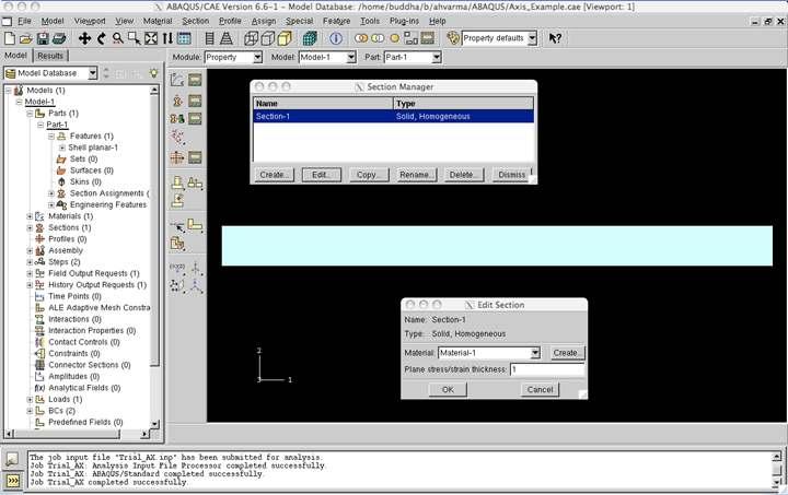
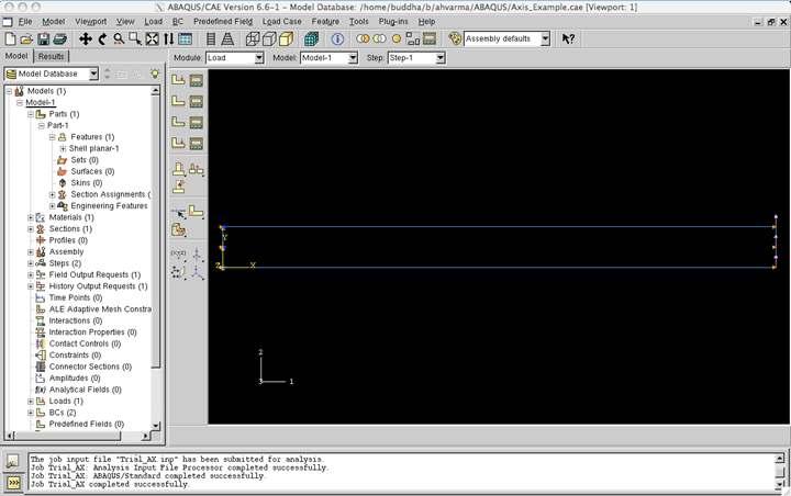
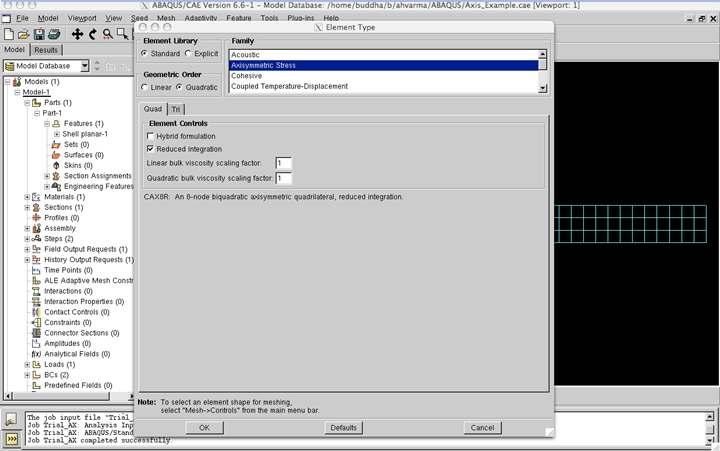
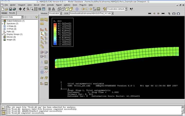
89 Example - Axisymmetric elements d 9 in. 123in. 1 ksi

90 Example

91 Example

92 Example

93 Example

94 Example

95 Example

96 Example

97 Example

98 Example

99 Example

100 Example

101