by Amy I. Hsieh B.Sc. (Earth Sciences), Simon Fraser University, 2013

Transcription

1 Geostatistical Modeling and Upscaling Permeability for Reservoir Scale Modeling in Bioturbated, Heterogeneous Tight Reservoir Rock: Viking Fm, Provost Field, Alberta by Amy I. Hsieh B.Sc. (Earth Sciences), Simon Fraser University, 2013 Thesis Submitted in Partial Fulfillment of the Requirements for the Degree of Master of Science in the Department of Earth Sciences Faculty of Science Amy I. Hsieh 2015 SIMON FRASER UNIVERSITY Summer 2015

2 APPROVAL Name: Degree: Title of Thesis: Examining Committee: Chair: Amy Hsieh Master of Science Geostatistical modeling and upscaling permeability for reservoir scale modeling in bioturbated, heterogeneous tight reservoir rock: Viking Fm, Provost Field, Alberta Dr. Andy Calvert Professor Dr. James MacEachern Senior Supervisor Professor Dr. Diana Allen Co-Supervisor Professor Dr. Shahin Dashtgard Supervisor Associate Professor By video conference from Edmonton Dr. Murray Gingras External Examiner Professor, University of Alberta Date Defended/Approved: August 13, 2015 _ ii

3 Abstract While burrow-affected permeability must be considered for characterizing reservoir flow, the marked variability generated at the bed/bedset scale makes bioturbated media difficult to model. Study of 28 cored wells of the Lower Cretaceous Viking Formation in the Provost Field, Alberta, Canada integrated sedimentologic and ichnologic features to define recurring hydrofacies possessing distinct permeability grades. Transition probability analysis was employed to model spatial variations in biogenically enhanced permeability at the bed/bedset scale. Results suggest that variations in permeability are strongly related to variations in hydrofacies rather than grain size. The variability in permeability at the bed/bedset scale was simplified by calculating an equivalent permeability that represents the thickness-weighted sum of permeability at the bed/bedset scale using expressions for layered media. Numerical block models were then generated for both the bed/bedset hydrofacies and the upscaled hydrofacies. Vertical and horizontal flows were simulated at both scales, and the volumetric flows in each direction were compared to verify the representativeness of the equivalent permeability. Vertical and horizontal flows simulated for bed/bedset scale and composite hydrofacies differ by less than 5%, suggesting that permeabilities at the bed/bedset scale can be simplified through upscaling. Reservoir-scale groundwater flow was simulated along a hydrogeological cross section comprised of the composite hydrofacies. The resulting flow regime was consistent with those simulated using permeability estimates from tight reservoir units of the Viking Formation. This approach may lead to improved reserve calculations, estimates of resource deliverability, and understanding of reservoir responses during recovery. Keywords: Bioturbation; Permeability; Statistical modelling; Upscaling; Numerical Modeling iii

4 Dedication To my Family iv

5 Acknowledgements I was lucky to have not one, but two amazing supervisors, Dr. James MacEachern and Dr. Diana Allen, who continuously guided me throughout the last two years. Thank you both for your patience, expertise, critiques, and most of all for strengthening my love of science. I would also like to thank Dr. Shahin Dashtgard and Dr. Murray Gingras for their insights and suggestions for my thesis, and Kevin Gillen for his motivation and assistance in the analyses of data. A very big thank-you goes to my amazing GRRG and ARISE lab mates for all the fun over the past two years, and especially for your incredible support during the stressful times that made my hair fall out. I am truly grateful for having you as lifetime friends. Also, Glenda Pauls, Tarja Vaisanen, Rodney Arnold, and Matt Plotnikoff are thanked for their endless dedication to the Earth Sciences Department. Finally, I would like to thank my family for their unconditional support and trust. Thank you for encouraging me to go off the beaten path v

6 Table of Contents Approval... ii Abstract... iii Dedication... iv Acknowledgements... v Table of Contents... vi List of Tables... viii List of Figures... ix List of Acronyms...xiv Chapter 1. Introduction Research Goals and Objectives Scope of Work Overview of Methodology Study Area Geologic Setting Background Biogenic Modification of Porosity and Permeability Vertical Transition Probability/Markov Chain Analysis Reservoir-Scale Modeling Chapter 2. Defining Hydrofacies at Different Scales Logging Permeability Data Bed to Bedset Scale HFs CHFs Descriptions and Process Interpretations CHF 1: Apparently structureless mudstone with siltstone to sandstone interbeds/interlaminae CHF 2: Bioturbated silty to sandy mudstone CHF 3: Bioturbated muddy to silty sandstone CHF 4: Interbedded mudstone and silty sandstone CHF 5: Sandstone with mudstone interlaminae/interbeds Stratigraphic Cross Sections Chapter 3. Statistical Modeling of Biogenically Enhanced Permeability in Tight Reservoir Rock Introduction Geologic Setting Geostatistics Methodology Logging Permeability Data Hydrofacies and Parameter Class Divisions Transition Probability Analysis vi

7 3.5. Results and Discussion Hydrofacies Transition Probability (Markov Chain) Analyses Conclusions Chapter 4. Upscaling Permeability for Regional Flow Modeling Average Hydraulic Conductivity for Bed to Bedset Scale HFs Hydraulic Conductivity Estimation for Composite HFs Validation of Equivalent K Regional Flow Simulations CHF Model Setup Additional Simulations Based on Literature K Values CHF Simulation Results Results of Flow Simulations using Literature K Values Discussion Chapter 5. Conclusions Hydrofacies Transition Probability Analysis Validation of Equivalent K Regional Flow Simulations Limitations Final Remarks References Appendix A. AccuMap Data Appendix B. Log Data and Geophysical Well Logs Appendix C. Horizontal Equivalent K Appendix D. Vertical Equivalent K vii

8 List of Tables Table 2.1. Table 3.1. Table 4.1. Bed/bedset scale hydrofacies descriptions. The calculated k ave (md) or representative k ave based on previous studies for each HF are also reported Bed/bedset scale hydrofacies descriptions. The calculated k ave (md) or representative k ave based on previous studies for each HF are also reported Bed/bedset scale hydrofacies identified in core and the calculated average hydraulic conductivity (K ave ) in m/s or representative K ave based on previous studies for HF 1. K ave values calculated in Chapter 3 are also shown below Table 4.2. Minimum, maximum, and average horizontal (K h ) and vertical (K v ) conductivities for each composite hydrofacies Table 4.3. Table 4.4. Table 4.5. Hydraulic conductivity (K) values of the Viking Formation measured in published literature, including the measurement techniques used as well as the lithology in which the measurements were taken Global water balance, average hydraulic flux (q) and average hydraulic conductivity (K) from the MODFLOW simulation over cross-section B-B Hydraulic flux (q) values calculated from MODFLOW results using hydraulic conductivity (K) values published in literature viii

9 List of Figures Figure 1.1. Flow chart of the methodologies used in this thesis Figure 1.2. Figure 1.3. Figure 1.4. Figure 1.5. Figure 2.1. Map of the study area showing the locations of the wells and cross sections Map showing the major hydrocarbon-producing fields of the Viking Formation in Alberta (MacEachern et al. 1999) Stratigraphic correlation diagram of the Viking Formation in central Alberta showing the overlying Westgate Formation, underlying Joli Fou Formation, as well as its stratigraphic equivalents, the Paddy Member and Bow Island Formation (MacEachern et al., 1999) Sand-filled trace fossils, such as Thalassinoides (Th) and Planolites (Pl) create potential flow paths in an otherwise lowpermeability unit. Mud-filled traces are dominated by Phycosiphon (Ph) Schematic diagram of the bioturbation index (BI), modified from Reineck (1963), Taylor and Goldring (1993) and Taylor et al. (2003) by MacEachern and Bann (2008). Bioturbation grades correspond to: BI 0 = 0% bioturbation; BI 1 = 1-5% bioturbation; BI 2 = 6-30% bioturbation; BI 3 = 31-60% bioturbation; BI 4 = 61-90% bioturbation; BI 5 = 91-99% bioturbation; and BI 6 = 100% Figure 2.2. log of PCP Verger W Figure 2.3. Figure 2.4. Examples of hydrofacies. A) Hydrofacies 3, 4, and 5 with Phycosiphon (Ph), Planolites (P), Scolicia (Sc), Asterosoma (As), and Schaubcylindrichnus (Sch). HF 5 exhibits planar parallel laminae. B) HF 2 with Chondrites (Ch), Asterosoma (As), and Phycosiphon (Ph) interbedded with laminated HF 4 containing Asterosoma (As) and fugichnia (fu). C) Wave ripple laminated HF 5 overlying HF 3 and HF 1. Trace fossils in HF 3 include Phycosiphon (Ph) and Schaubcylindrichnus (Sch). D) HF 5 and HF 4 interbedded with HF 1. Trace fossils in HF 4 include Asterosoma (As) and Phycosiphon (Ph). Trace fossils in HF 1 include Planolites (P) and Chondrites (Ch) Examples of CHF 1. A) Mudstone showing BI 0-2, with interbedded wavy laminated silty sandstone. Trace fossils include Schaubcylindrichnus freyi (Sf), Phycosiphon (Ph), Asterosoma (As), and Chondrites (Ch). B) Bentonitic mudstone displaying BI 0-1, with laminated silty sandstone lenses. Trace fossils include Chondrites (Ch), Planolites (P), and Asterosoma (As). C) Mudstone showing BI 0-2 with interbedded HCS to planar parallel laminated sandstone and silty sandstone layers. Trace fossils include fugichnia (fu), Chondrites (Ch), Asterosoma (As), and Phycosiphon (Ph) ix

10 Figure 2.5. Examples of CHF 2. A) Bioturbated silty to sandy mudstone (BI 4) with interbedded structureless mudstone and laminated to structureless sandstone. Trace fossils include Chondrites (Ch), Planolites (P), Asterosoma (As), Diplocraterion (D), Phycosiphon (Ph), Schaubcylindrichnus freyi (Sf), and Zoophycos (Z). B) Bioturbated silty to sandy mudstone (BI 4-5) with interbedded structureless mudstone. Trace fossils include possible Diplocraterion (D?), Chondrites (Ch), Schaubcylindrichnus freyi (Sf), Teichichnus (T), Zoophycos (Z), and Planolites (P). C) Bioturbated silty to sandy mudstone (BI 4-5) with interbedded structureless mudstone. Trace fossils include Planolites (P), Phycosiphon (Ph), possible Diplocraterion (D?), possible Thalassinoides (Th?), Helminthopsis (H), and Asterosoma (A). D) Bioturbated silty to sandy mudstone (BI 4-5) with interbedded structureless mudstone and laminated to structureless sandstone. Trace fossils include Schaubcylindrichnus freyi (Sf), Planolites (P), Chondrites (Ch), Rosselia (Ro), Phycosiphon (Ph), and Asterosoma (As). E) Bioturbated silty to sandy mudstone (BI 5). Trace fossils include Thalassinoides (Th), Zoophycos (Z), Asterosoma (As), Planolites (P), Phycosiphon (Ph), Schaubcylindrichnus freyi (Sf), and Chondrites (Ch) Figure 2.6. Examples of CHF 3. A) Lower very fine- to lower fine-grained bioturbated muddy to silty sandstone. Units show BI 4-5. Trace fossils include Asterosoma (As), Planolites (P), Zoophycos (Z), Phycosiphon (Ph), Schaubcylindrichnus freyi (Sf), and Diplocraterion (D). B) Lower fine-grained bioturbated silty sandstone (BI 4-5) with interbedded mudstone and laminated sandstone. Trace fossils include Palaeophycus (Pa), Asterosoma (As), Planolites (P), Siphonichnus (Si), Chondrites (Ch) and fugichnia (fu). C) Lower fine-grained bioturbated muddy to silty sandstone (BI 4-5) with interbedded mudstone and laminated sandstone. Trace fossils include Schaubcylindrichnus freyi (Sf), Chondrites (Ch), Teichichnus (T), Asterosoma (As), Planolites (P), Diplocraterion (D), Palaeophycus (Pa), and Thalassinoides (Th). D) Lower fine-grained bioturbated muddy to silty sandstone (BI 5). Trace fossils include Diplocraterion (D), Phycosiphon (Ph), Planolites (P), Rhizocorallium (Rh), Chondrites (Ch), and Asterosoma (As). E) Lower very fine-grained bioturbated muddy to silty sandstone (BI 4-5). Trace fossils include Schaubcylindrichnus freyi (Sf), Chondrites (Ch), Phycosiphon (Ph), Planolites (P), Teichichnus (T), and Asterosoma (As). F) Lower fine-grained bioturbated silty sandstone (BI 4-5) with interbedded mudstone and laminated sandstone. Trace fossils include Phycosiphon (Ph), Schaubcylindrichnus freyi (Sf), Chondrites (Ch), Planolites (P), and Rosselia (Ro) x

11 Figure 2.7. Figure 2.8. Figure 2.9. Figure Figure 3.1. Figure 3.2. Figure 3.3. Figure 3.4. Examples of CHF 4. A) Interbedded mudstone and silty sandstone. The mudstone beds are structureless, and the sandstone beds exhibit planar parallel laminae. Units show BI 0-2. The trace -fossil suite includes Thalassinoides (Th), Chondrites (Ch), Diplocraterion (D), Planolites (P), and Phycosiphon (Ph). B) Apparently structureless mudstone, interbedded with planar parallel to wavy laminated silty sandstone. Bioturbation intensities range from BI 0-3. Trace fossils include fugichnia (fu), Planolites (P), Phycosiphon (Ph), Chondrites (Ch), and possible Skolithos (Sk?). C) Interlaminated mudstone and silty sandstone with bentonite cementation. Units show BI 0-1. Trace fossils are diminutive and include Planolites (P), Chondrites (Ch), and Phycosiphon (Ph). D) Apparently structureless mudstone interbedded with laminated silty sandstone Examples of CHF 5. A) Lower medium-grained sandstone with low-angle planar parallel laminae and possible cryptic bioturbation. B) Wavy laminated, upper fine-grained sandstone. Unit shows BI 0-1. Trace fossils include Chondrites (Ch) and Zoophycos (Z). C) Lower medium-grained sandstone with HCS. The rip-up clast (rc) layer in the photo is likely composed of eroded and transported fragments of Rosselia, Palaeophycus, or Asterosoma. D) Lower medium-grained sandstone. The tracefossil suite includes Rosselia (Ro), possible Asterosoma (As?), Chondrites (Ch), Skolithos (Sk), Planolites (P), and Phycosiphon (Ph) Stratigraphic cross-section A-A constructed using composite hydrofacies (CHF) Stratigraphic cross-section B-B constructed using composite hydrofacies (CHF) Sand-filled trace fossils such as Thalassinoides (Th) and Planolites (Pl) create potential flow paths in an otherwise lowpermeability unit. Mud-filled traces are dominated by Phycosiphon (Ph) Map showing the major hydrocarbon-producing fields of the Viking Formation in Alberta (MacEachern et al., 1999) Stratigraphic correlation diagram of the Viking Formation in central Alberta showing the overlying Westgate Formation, underlying Joli Fou Formation, as well as its stratigraphic equivalents, the Paddy Member and Bow Island Formation (MacEachern et al., 1999) Schematic diagram of the bioturbation index (BI), modified from Reineck (1963), Taylor and Goldring (1993) and Taylor et al. (2003) by MacEachern and Bann (2008). Bioturbation grades correspond to: BI 0 = 0% bioturbation; BI 1 = 1-4% bioturbation; BI 2 = 5-30% bioturbation; BI 3 = 31-60% bioturbation; BI 4 = 61-90% bioturbation; BI 5 = 91-99% bioturbation; and BI 6 = 100% xi

12 Figure 3.5. Example of a Markov chain transiogram. The transition probability value at which the curve reaches its limit is the sill. The lag distance at which the Markov chain reaches the sill is the range. The slope of the tangent line is the transition rate of the material, and the point at which the tangent line intersects the x-axis is the mean les length of the material Figure 3.6. log of PCP Verger W Figure 3.7. Figure 3.8. Figure 3.9. Figure 4.1. Examples of hydrofacies. A) Hydrofacies (HF) 3, 4, and 5 with Phycosiphon (Ph), Planolites (P), Scolicia (Sc), Asterosoma (As), and Schaubcylindrichnus (Sch). HF 5 exhibits planar parallel laminae. B) HF 2 with Chondrites (Ch), Asterosoma (As), and Phycosiphon (Ph) interbedded with laminated HF 4 containing Asterosoma (As) and fugichnia (fu). C) Wave ripple laminated HF 5 overlying HF 3 and HF 1. Trace fossils in HF 3 include Phycosiphon (Ph) and Schaubcylindrichnus (Sch). D) HF 5 and HF 4 interbedded with HF 1. Trace fossils in HF 4 include Asterosoma (As) and Phycosiphon (Ph). Trace fossils in HF 1 include Planolites (P) and Chondrites (Ch) Vertical transition probability matrix for k max (solid black line) vs. grain size (dashed gray line). fl: lower fine-grained; fu: upper fine-grained; ml: lower medium-grained Vertical transition probability matrix for k max (solid black line) vs. hydrofacies (dotted gray line) Upscaling hydraulic conductivity (K) at the bed to bedset scale to a single equivalent hydraulic conductivity in both the vertical (K v ) and horizontal (K h ) directions for a composite hydrofacies using the expressions for layered media (see Equations 4.1 and 4.2) Figure 4.2. Boundary conditions for A) horizontal flow simulations and B) vertical flow simulations. h refers to the assigned hydraulic head Figure 4.3. Figure 4.4. Figure 4.5. Figure 4.6. A) Example of a MODFLOW block model of a cored section with hydrofacies logged at the bed/bedset scale. Each colour represents a different hydrofacies. B) Block model of the same cored section with hydrofacies logged at the composite scale Discharge in Q (m 3 /s) for bed/bedset scale and composite scale fluid flow simulations in the A) horizontal and B) vertical directions Hydrogeological cross-section B-B constructed using Composite Hydrofacies (CHF) Contours of hydraulic head in the Viking Formation, showing the locations of cross-sections A-A and B-B. Contour intervals are in metres. The solid black arrow shows the simplified direction of the groundwater flow, and the dotted gray arrows show actual groundwater flow directions (Modified after Bachu et al., 2002). Estimates of the hydraulic head are shown for the ends of each cross section xii

13 Figure 4.7. Figure 4.8. Figure 4.9. Figure MODFLOW domain for hydrogeological cross-section B-B showing the hydraulic heads (h) at the NW and SE boundaries Equipotential head contour map of cross-section B-B. Contour units are in metres. The zoomed section illustrates the deviation of flow lines in red arrows. The maximum arrow length corresponds to a maximum velocity of m/s, to which all other vectors are scaled Fluid flow velocity vector map for cross-section B-B. The maximum arrow length corresponds to a maximum velocity of m/s, to which all other vectors are scaled Distribution of hydraulic flux (q) values calculated using ranges of Viking Formation hydraulic conductivities found in literature. The q from the CHF simulation falls between and m/s xiii

14 List of Acronyms BI CHF fl fu GMS h HCS HF K k ave K ave K h k max K v ml Q q rc T-PROGS Bioturbation Index (grades of bioturbation intensity) Composite hydrofacies Lower fine-grained Upper fine-grained Groundwater Modelling Software Hydraulic head Hummocky cross-stratification Hydrofacies Hydraulic conductivity Average permeability Average hydraulic conductivity Horizontal hydraulic conductivity Maximum permeability Vertical hydraulic conductivity Lower medium-grained Discharge Darcy flux Rip-up clast Transition Probability Geostatistical Software Trace Fossils As Asterosoma Ch Chondrites D Diplocraterion fu fugichnia P Planolites Pa Palaeophycus Ph Phycosiphon Rh Rhizocorallium Ro Rosselia Sc Scolicia xiv

15 Sch Sf Sk T Th Z Schaubcylindrichnus coronus Schaubcylindrichnus freyi Skolithos Teichichnus Thalassinoides Zoophycos xv

16 Chapter 1. Introduction The storage capacity and productivity of a reservoir are determined by its porosity and permeability. Permeability is also an important factor that controls reservoir response during enhanced hydrocarbon recovery. Correspondingly, understanding and projecting variations in porosity and permeability within a reservoir are vital to maximizing the acquisition of the resource. Recently, there has been considerable interest in recovering hydrocarbons from marginal (generally lower-quality) reservoirs using horizontal drilling techniques and fracturing, particularly in areas prone to light oil. The so-called Tight Oil play of the Viking Formation in east-central Alberta and westcentral Saskatchewan constitutes one example. Tight reservoirs are characterized by permeabilities that range from md (Spencer, 1989; Holditch, 2006; Clarkson and Pedersen, 2010). In such reservoirs, subtle changes in the distribution of sedimentary media, such as that generated by bioturbation, can greatly affect the porosity and permeability distribution of the facies. Bioturbation remains an under-appreciated mechanism by which porosity and permeability of a sedimentary facies are modified (cf. Pemberton and Gingras, 2005). Even when considered, bioturbation is generally perceived to be detrimental to bulk permeability, through reduction of primary grain sorting, homogenization of the sediment, and introduction of mud through linings, biogenic deposits, and feces (Qi, 1998; Dornbos et al., 2000; Qi et al., 2000; McDowell et al., 2001; Pemberton and Gingras, 2005; Tonkin et al., 2010; Lemiski et al., 2011; La Croix et al., 2013). Recent studies have shown, however, that several ichnogenera and their associated biogenic fabrics are capable of increasing a reservoir rock s porosity and permeability (Gingras et al., 2004; Pemberton and Gingras, 2005; Hovikoski et al., 2007; Volkenborn et al., 2007; Cunningham et al., 2009; Tonkin et al., 2010; Lemiski et al., 2011; Gingras et al., 2012; 1

17 La Croix et al., 2013; Knaust, 2014). Ichnogenera that form branching burrow networks can create flow pathways in otherwise less permeable units where the burrow fills consist of coarser grains and better-connected intergranular pore space relative to the surrounding matrix (Gingras et al., 2004; Pemberton and Gingras, 2005; Lemiski et al., 2011; Gingras et al., 2012; La Croix et al., 2013). Additionally, burrows are capable of increasing vertical permeability in laminated sedimentary rocks where horizontal permeability tends to dominate (Gingras et al., 2012). Burrow fills also may undergo diagenetic changes that may lead to higher permeability than that of the surrounding matrix (Pemberton and Gingras, 2005; Tonkin et al., 2010; Gingras et al., 2012). Despite increasing evidence of biogenic enhancement of permeability and porosity, permeability across unfractured sedimentary reservoirs is commonly assessed solely on the basis of average grain size (e.g., lithostratigraphic units). Indeed, bioturbation is generally neglected in permeability assessments of rock units owing to the complexity of bioturbated media (Gingras et al., 2012). Unless bioturbation intensities are high, and the burrows are filled with (i) a contrasting lithology, (ii) coarser sediment, or (iii) media with different degrees of sorting relative to the surrounding matrix (e.g., abundant mud-filled traces in a sandstone matrix), burrowed and unburrowed units are assigned the same permeability values. This is particularly problematic in tight oil/gas reservoirs, where even small disturbances in the sedimentary fabric caused by bioturbation can significantly increase permeability in these otherwise impermeable units (e.g., Pemberton and Gingras, 2005; Hovikoski et al., 2007; Gingras et al., 2012; La Croix et al., 2013; Knaust, 2014). While burrow-affected permeability trends in reservoirs must be considered in order to properly characterize reservoir parameters, the marked variability generated at the bed to bedset scale makes such bioturbated media difficult to model. To simulate flow in such heterogeneous media, the spatial variations in hydraulic conductivity must be characterized accurately to simulate the true geologic and hydrogeologic heterogeneities that are observed and measured in core (Park et al., 2004). Instead of defining permeability on the basis of average grain size alone, herein the use of hydrofacies (HF) in reservoir characterization is proposed. Such a hydrofacies is 2

18 defined as a recurring unit possessing a distinct permeability that is associated with a combination of sedimentological and ichnological characteristics. To analyze vertical and lateral facies relationships, and to characterize subsurface heterogeneities and uncertainties, geostatistical methods based on Walther s Law can be applied. Walther s Law states: The various deposits of the same facies area and similarly the sum of the rocks of different facies areas are formed beside each other in space, though in cross section we see them lying on top of each other. As with biotopes, it is a basic statement of far-reaching significance that only those facies and facies areas can be superimposed primarily which can be observed beside each other at the present time. (Walther, 1894 as translated by Middleton, 1973). This law implies that sedimentary environments tend to experience gradual spatial shifts with time (cf. Dalrymple, 2010). Thus, the occurrence of biogenically induced permeable layers may be statistically predictable by understanding the cyclic repeatability of sedimentary processes. Traditionally, geostatistical models such as variograms, coupled with data interpolation, have been used to simulate spatial variability in the hydraulic properties of geologic media. These methods, however, have strict requirements (e.g., Gaussian distribution, stationarity) that are unrealistic in geologic environments. In addition, these methods may generate results that are too smooth and continuous, particularly in datasparse areas (Park et al., 2004). Alternatively, a more intuitive, mathematically compact, and theoretically effective method was proposed by Carle and Fogg (1996) a transition probability approach coupled with Markov chain analysis which permits the integration and subjective interpretation of geologic data (Park et al., 2004). In this thesis, transition probability analysis is explored as a possible statistical tool for modeling the spatial variations in biogenically enhanced permeability at the small scale (bed and bedset scales as expressed in core), and for defining hydrofacies. An approach is tested for logging hydrofacies at a composite scale and assigned upscaled permeability values that can be used for reservoir-scale modeling. Such an 3

19 approach may lead to improved reserve calculations, estimates of resource deliverability, and understanding of reservoir response throughout all stages of recovery Research Goals and Objectives To characterize heterogeneous, tight reservoirs, it is necessary to consider not only the lithologic, but the biogenic and hydraulic properties of the facies as well. Different hydrofacies could be defined based on properties. The combination of these properties at the bed to bedset scale, which can be observed in core, then need to be upscaled in order to model permeability trends at the three-dimensional reservoir scale. This requires not only a means to map hydrofacies at the reservoir scale, but also a method to assign appropriate upscaled hydraulic properties to those composite hydrofacies. The purpose of this study is to explore the use of Markov transition probability analysis in combination with conventional core logging techniques and permeability data as a means for defining hydrofacies and their associated hydraulic properties at two scales: the bed to bedset scale and the composite scale. The study is focused on a biogenetically enhanced reservoir from the Viking Formation of the Provost Field, Alberta. The study integrates sedimentology, ichnology, hydrogeology, and geostatistics to characterize flow in bioturbated, heterogeneous media. The objectives of the research are: 1. To establish criteria that define hydrofacies (HF). 2. To explore the transition relations between permeability and various properties measureable at the bed/bedset and composite scales, including sedimentology and ichnology, as a means to identify which parameter (or combination of parameters) best reflects the permeability transitions. 3. To estimate and verify the equivalent permeability for each composite hydrofacies. 4. To test the use of upscaled composite hydrofacies for representing geological heterogeneity in a flow model. 4

20 1.2. Scope of Work The following tasks were undertaken for this research: Objective 1: 1. logging at the bed/bedset scale and composite scale of selected cores within the Viking Formation of the Provost Field, Alberta. 2. Defining different hydrofacies based on lithology, sedimentary structures, sedimentary accessories, ichnological suites, bioturbation index (BI), grain size, porosity, and permeability. Objective 2: 1. Using the T-PROGS software (GMS version 6.0, Copyright 2013 Aquaveo) to produce vertical transition probability matrices for permeability, average grain size, and bed/bedset hydrofacies to identify which parameter (or combination of parameters) best reflects the permeability transitions. Objective 3: 2. Estimating equivalent permeability for composite hydrofacies using the multi-layer equivalent permeability approach. 3. Generating block models using the defined bed/bedset scale and composite scale hydrofacies and their corresponding equivalent permeability values to evaluate whether the upscaled hydrofacies yield consistent results with the bed/bedset hydrofacies representations. Objective 4: 4. Constructing a cross section in the direction of the regional hydraulic gradient and the regional structural dip of the study area using the composite hydrofacies and their corresponding equivalent permeability values, and then simulating flow along the cross section using MODFLOW Overview of Methodology The methodology used in this research project involved a combination of steps as shown in Figure 1.1: 5

21 1. logging the bed to bedset scale and identification of bed to bedset scale hydrofacies (HFs). 2. Permeability analyses from plug and full-diameter core measurements (k max ). 3. Transition probability analysis for evaluating the bed to bedset scale HFs as an indicator of permeability. 4. Calculation of average hydraulic conductivities (K ave ) for each HF identified at the bed to bedset scale. 5. logging according to composite HFs. 6. Estimation of the upscaled equivalent hydraulic conductivity in both the horizontal (K h ) and vertical (K v ) directions for the composite HFs using the K ave values for the bed to bedset scale HFs. 7. Validation of the equivalent hydraulic conductivities using numerical flow modeling. 8. Regional numerical flow modeling along a cross section in the study area using the upscaled equivalent hydraulic conductivities for the composite HFs. 6

22 Figure 1.1. Flow chart of the methodologies used in this thesis. 7

23 1.4. Study Area The study area (Figure 1.2) for this research project lies within the Provost Field of southeastern Alberta, Canada. Twenty-nine cored sections of the Viking Formation were selected for this project. Wells of the Viking Formation were chosen because the hydrocarbon-producing successions in the area consist of tight sandstones that exhibit interlayering of impermeable and permeable beds with variable but locally pervasive bioturbation. The type, distribution, and intensity of bioturbation are influenced by both allogenic and autogenic variations in the sedimentary environment (e.g., MacEachern et al., 2010). The trace-fossil suites observed in the facies successions reflect proximaldistal as well as along-strike shifts in the causative environment. The cores selected were drilled post-1970s, have core analysis data, and extend for two townships and three ranges in area (TP 34-35, R08-10W4M; representing and area of approximately 530 km 2 ). 8

24 Figure 1.2. Map of the study area showing the locations of the wells and cross sections. 9

25 1.5. Geologic Setting The Lower Cretaceous (Upper Albian) Viking Formation is a prolific oil- and gasproducing interval that was deposited in the Western Canada foreland basin during a period of active tectonism and eustatic sea level fluctuations. During Viking deposition, a shallow epicontinental seaway extended from the Arctic Ocean to the Gulf of Mexico (Figure 1.3; Williams and Stelck, 1975; Caldwell, 1984; Walker, 1990; Reinson et al., 1994), into which was deposited a complex succession of mudstones, heterolithic bedsets of sandstone and shale, sandstones, and minor conglomerates. Figure 1.3. Map showing the major hydrocarbon-producing fields of the Viking Formation in Alberta (MacEachern et al. 1999). The Viking Formation stratigraphically overlies the Joli Fou Formation and underlies the Westgate Formation (Figure 1.4; Stelck, 1958). It is generally regarded to be roughly equivalent to the Paddy Member of the Peace River Formation of 10

26 northwestern Alberta (Leckie et al., 1990), and the Bow Island Formation of southern Alberta and southwestern Saskatchewan (Figure 1.4; Stelck and Koke, 1987; Raychaudhuri and Pemberton, 1992). The stratigraphic relationships were addressed by the work of Stelck (1958), Glaister (1959), McGookey et al. (1972), Weimer (1984), Cobban and Kennedy (1989), Stelck and Leckie (1990), Bloch et al. (1993), Caldwell et al. (1993), and Obradovich (1993). Figure 1.4. Stratigraphic correlation diagram of the Viking Formation in central Alberta showing the overlying Westgate Formation, underlying Joli Fou Formation, as well as its stratigraphic equivalents, the Paddy Member and Bow Island Formation (MacEachern et al., 1999). The Upper Albian Viking Formation comprises a siliciclastic succession mainly reflecting shoreface, delta and estuarine incised valley deposits (cf. Boreen and Walker, 1991; Pattison, 1991; Pattison and Walker, 1994; Reinson et al., 1994; Walker, 1995; Burton and Walker, 1999; MacEachern et al., 1999; Dafoe et al., 2010). These clastic sediments were supplied from the rising Cordillera in the west and reflect northward and eastward progradation of environments into the Alberta foreland basin. 11

27 Despite the Viking deposits only ranging from 15 to 30 m in thickness, they are discontinuity bound and depositionally complex, resulting in sedimentary successions, facies, and geometries that are challenging to characterize and correlate. Beaumont (1984), Boreen and Walker (1991), Pattison (1991), Posamentier and Chamberlain (1993), Reinson et al. (1994), Pattison and Walker (1994), Walker (1995), Burton and Walker (1999), and MacEachern et al. (1999), among others, have attempted to provide allostratigraphic and sequence stratigraphic assessments of the Viking, with varying levels of success. Viking Formation discontinuities have been linked to the global changes of sea level outlined in Kauffman (1977), Vail et al. (1977), Weimer (1984), and Haq et al. (1987). A cored interval of the Viking Formation from the Verger Field was selected for this study because it exhibits stacked parasequences characterized by the interstratification of impermeable and permeable beds with variable but locally pervasive bioturbation Background Biogenic Modification of Porosity and Permeability Bioturbation is the modification of sedimentary media by epifaunal and/or endobenthic organisms. It includes tracks, trails, burrows, feeding structures, and escape structures. These features are not the organisms themselves, but instead a record of the organisms activities in the environment. The distribution of trace-fossil assemblages is largely controlled by complex environmental factors, including sediment type, substrate consistency, sediment grain size, food-resource types, energy conditions, salinity, oxygenation, water turbidity, and deposition rate (e.g., Ekdale et al., 1984; Pemberton et al., 1992; MacEachern et al., 2005; Gingras et al., 2007). Softground trace-fossil assemblages reflect the condition(s) of the sedimentary environment in which the trace-making animals lived. Organisms and their corresponding burrowing behaviours are extremely sensitive to changes in their habitats and, as a result, trace fossils provide excellent indicators of changing depositional conditions at various temporal scales. 12

28 In sedimentary geology, autogenically induced sedimentary cycles are depositional events that recur within a single sedimentary system and result from changes that are intrinsic to the system (cf. Beerbower, 1964; Cecil, 2003). The effects of these autogenic events tend to range from local to regional (e.g., from current ripple migration through channel migration, to avulsion-driven delta lobe switches or lateral shifts of submarine fan lobes). These events may be periodic and occur geologically instantaneously (Reading, 1996). Allogenically induced sedimentary cycles, on the other hand, comprise recurring events that are imposed externally on the sedimentary system (cf. Beerbower, 1964; Cecil, 2003). Examples of allogenic events include effects of climate change, Milankovitch processes and orbital forcing, and tectonically or eustatically driven sea-level changes, although the latter two are more aperiodic (Reading, 1996). Progressive recurring changes in depositional conditions owing to shifts of environments (either autogenically or allogenically induced) can be marked by cyclic changes in the resulting rock properties (e.g., Bernard and Major, 1963; Krumbein and Sloss, 1963; Beerbower, 1964; Reading, 1996). This includes changes in bioturbation intensity and trace-fossil assemblages (e.g., Pemberton et al., 1992; Taylor et al., 2003; McIlroy, 2004; MacEachern et al., 2010). It is generally assumed that bioturbation reduces porosity and permeability by altering grain sorting, disturbing primary sedimentary layering, "piping" sediment and fluids between sedimentary units, adding or removing organic matter and clay, creating pathways for mineralizing pore fluids, or changing pore fluid chemistries (e.g., McDowell et al., 2001; Pemberton and Gingras, 2005; Tonkin et al., 2010). By contrast, some studies have shown that bioturbation is capable of enhancing bulk permeability and vertical permeability in otherwise impermeable or marginally permeable rock units (e.g., Gingras et al., 1999; Pemberton and Gingras, 2005; Gingras et al., 2007; Tonkin et al., 2010; Baniak et al., 2012). For example, in their study of the Upper Cretaceous Medicine Hat Formation of Alberta, Canada, La Croix et al. (2013) demonstrated that several ichnogenera served to improve permeability by approximately two orders of magnitude compared to the unburrowed matrix. In the Upper Triassic Montney Formation of northeastern British Columbia and the Upper Cretaceous Alderson Member of southwestern Saskatchewan, spot 13

29 permeability tests show that small and interconnected Phycosiphon are associated with increased porosity and permeability values ( md) compared to those of the surrounding matrix ( md; Hovikoski et al., 2007 and Lemiski et al., 2011, respectively). These studies show that bioturbation is analogous to natural fractures, with large surface areas capable of enhancing flow within lower permeability units (Lemiski et al., 2011). Volkenborn et al. (2007) provide a modern analogue of biogenically enhanced permeability by the burrowing of lugworms (Arenicola marina). This large-scale experiment of lugworms in 400 m 2 of intertidal fine-grained sand showed that not only are these polychaetes capable of significantly increasing porosity and permeability by creating flow paths through their burrows, but that a lack of these infauna resulted in an influx of organic particles that obstructed the pores, causing an eight-fold decrease in permeability. These results show the effectiveness of bioturbation in creating and maintaining a permeable condition within some sedimentary facies (Volkenborn et al., 2007). Examples of biogenically enhanced reservoirs also include the Biscayne aquifer in Florida (Cunningham et al., 2009) and the Ghawar Field of Saudi Arabia (Pemberton and Gingras, 2005). The highly permeable layers of the Biscayne aquifer (known as Super K zones) are the result of Thalassinoides- and Ophiomorpha-induced macroporosity networks, coupled with minor moldic porosity from the dissolution of fossils (Figure 1.5; Cunningham et al., 2009). The Hawiyah portion of the Ghawar Field in Saudi Arabia also exhibits such Super K zones, generated by firmground (palimpsest) Thalassinoides boxworks filled with detrital sucrosic dolomite (Pemberton and Gingras, 2005). These palimpsest burrows have diameters ranging from 1 2 cm and lengths of up to 2.1 m (La Croix et al., 2013). Permeable flow paths created by bioturbation result from lithological contrast between the trace-fossil fill and the rock matrix (Figure 1.5), changes in sorting, and/or geochemical heterogeneities within the matrix (Tonkin et al., 2010). Biogenic flow paths occur in both clastic and carbonate reservoirs, wherein burrow fills consist of differing lithologies, sediment calibres, or degrees of sorting relative to those of the host 14

30 substrate; and correspondingly may be subject to different diagenetic processes (Pemberton and Gingras, 2005). Figure 1.5. Sand-filled trace fossils, such as Thalassinoides (Th) and Planolites (Pl) create potential flow paths in an otherwise low-permeability unit. Mudfilled traces are dominated by Phycosiphon (Ph). The morphology and density of traces constitute important factors in the resulting porosity and permeability distributions (La Croix et al., 2013). For example, whereas both Ophiomorpha and Thalassinoides tunnels are large in diameter and prone to branching geometries, laboratory analyses show that Ophiomorpha may be less effective at enhancing permeability and may even reduce permeability owing to their pelleted mud linings (Tonkin et al., 2010). In addition to the density of bioturbation and size of burrows, the geometry of the ichnogenera can affect the connectivity of flow pathways. Burrows that branch both vertically and horizontally such as Thalassinoides are more effective in creating an isotropic flow network (La Croix et al., 2013). Trace fossils that do not branch, such as Skolithos, rely on chance interpenetrations to connect 15

31 individual flow paths. Cryptobioturbation results in such thoroughly interconnected flow paths that the entire rock body can be considered to be essentially isotropic (La Croix et al., 2013). Elevated bioturbation intensities associated with permeability-enhancing burrows can result in higher effective porosities by increasing the number of permeable flow pathways and/or by enhancing burrow interpenetrations, leading to more continuous flow paths (La Croix et al., 2013). Bioturbated dual-porosity systems are regarded as those where most of the rock volume conducts flow and the permeability of the matrix lies within two-orders of magnitude of the burrow permeability (Gingras et al., 2004). Such dual-porosity scenarios are generally created by the movement of organisms through the sediment, by sand-dwelling organisms that ingest sediment and rework the deposits, through passive filling or active backfilling of burrows with coarser grains, and (in carbonates) burrow-associated diagenesis (Gingras et al., 2004, 2012; La Croix et al., 2013). Common burrow fabrics that are associated with the generation of dual-porosity systems include cryptobioturbation, pervasive burrowing with Macaronichnus, and suites with abundant ichnogenera such as Thalassinoides, Zoophycos, Planolites, Ophiomorpha, Skolithos, and Arenicolites (e.g., Pemberton and Gingras, 2005; Gingras et al., 2012; La Croix et al., 2013). In sedimentary media where the matrix permeability is three-orders of magnitude or higher or lower than that of the burrow permeability, the system has been termed a dual-permeability network (see Gingras et al., 2004; Pemberton and Gingras, 2005; Gingras et al., 2012) Vertical Transition Probability/Markov Chain Analysis To determine the strength of the relationship between permeability and each of the logged parameters (e.g., grain size, BI, porosity, and HF) at the bed/bedset scale, vertical transition probability analyses were undertaken. Using this method, the probability of each class passing upwards into another was calculated using the Transition Probability Geostatistical Software (T-PROGS) developed by Carle (1999) within the Groundwater Modelling Software (GMS version 6.0, 2013 Aquaveo). 16

32 The transition probability method is a modified form of indicator kriging that can simulate spatial heterogeneity in subsurface geology (Park et al., 2004). A two- or threedimensional Markov chain model is developed using measurable geologic and/or hydraulic properties, such as volumetric proportions, mean lens lengths, and juxtapositional relationships that are estimated using the transition probability approach (Park et al., 2004). In a geologic sense, the transition probability approach assumes the sedimentary rock type that occurs in a stratigraphic column depends solely upon the type of rock preserved directly below the interval of interest, and not on rock types preserved sequentially below that (Jones et al., 2003). For example, in a prograding shoreface environment, one would expect to find a gradual upward-coarsening succession of facies. If the rock type observed is fine-grained laminated sandstone of the middle shoreface, the unit that is mostly likely to occur above this is medium-grained crossstratified sandstone of the upper shoreface, regardless of what rock type was deposited before the fine-grained laminated sandstone. In terms of spatial distributions, the probability of occurrence of a class (e.g., rock type) is dependent upon the nearest occurrence of another class over a specified lag interval. The probability of class 1 passing into class 2 can be defined by: p 12 h Φ = Pr{(class 2 occurs at x + h Φ ) (class 1 occurs at x)} (1.1) where h Φ represents the lag distance in the direction Φ (Carle, 1999). The spatial correlation among different sedimentary facies can be calculated using a Markov chain analysis; a mathematical model that transitions from one state to another between a fixed number of possible discrete states (Carle, 1999). For example, a succession of sedimentary facies may be characterized by a preferred tendency for sediment A to be deposited after sediment B, but not sediment C. Therefore, the spatial occurrence of sediment A may be dependent on the pre-existence of sediment B but independent of sediment C (Li et al., 2005). Additionally, if sediments A, B, and C tend to be deposited upwards as a sequence ABC, this asymmetric relationship also can be characterized using Markov chain analysis (Li et al., 2005). 17

33 The Markov chain is described as follows: There are a set of classes, S = {s 1, s 2,, s r }, that pass sequentially from one to another in steps. The probability of class s 1 moving to class s 2 is represented by p 12, otherwise known as the transitional probability from s 1 to s 2. If the transition remains in the same class s 1, it is denoted by the probability p 11 (Grinstead and Snell, 1997). For example, Carle (1999) assessed the transition probabilities down a well log using an embedded analysis of the Markov chain with respect to a matrix of vertical transitions from one discrete sedimentary facies to another. In that study, an embedded Markov chain analysis of a vertical succession was defined by three facies (A, B, and C) according to the following steps (Carle, 1999): 1. Disregard the lag or spatial dependency and relative thicknesses of the beds. 2. Log the embedded occurrences of A, B, and C down the borehole (e.g., ABCABACABCABABC). 3. Count the number of transitions from one state to another in a transition count matrix. A B C A B 2-3 C Self-transitions (e.g., from A to A) are unobservable in single or stacked beds, and are therefore blank (null) in the transition matrix. 4. Divide each transition count by the sum of the row to find the embedded transition probabilities. A B C A B C This final matrix shows the transition probabilities for each combination of units. Diagonal elements are self-transition probabilities within a category (A to A, B to B, C to C), and the off-diagonal elements are the probabilities of transition between categories (i.e. cross-transition, Carle, 1999) 18

34 The Markov transition probability approach is generally useful for stratigraphically confined simulations. As is clearly stated in Walther s Law, genetic and predictable relationships exist for facies successions that occur between stratigraphic breaks, and are absent in facies separated by such breaks. Markov transition probability can be used to demonstrate the lack of correlatibility of facies across such stratigraphic breaks (Weissmann, 2005). Another advantage of using Markov chain models is that the simulation assumes stratigraphic stationarity (statistical homogeneity; i.e., the mean and standard deviation do not change over time or space) across the modeled reservoir (Weissmann, 2005). In other words, by dividing the vertical stratigraphic succession in a core into facies, the proportions and geometries of different facies within the environment are maintained. In a transgressive marine environment, for example, the proportion of fine-grained facies is higher than coarse-grained facies across the environment, and the probability of fine-grained facies being deposited is likewise greater. This ensures that the facies represented in the model is not a result of random variables, but instead is reflective of the character of the depositional conditions. Further, the distribution of facies within the stratigraphic unit theoretically can be simulated, resulting in a quantifiable conceptual model that facilitates the interpretation of the reservoir s heterogeneity (Weissmann, 2005) Reservoir-Scale Modeling Reservoir-scale modeling involves the simulation of both vertical and lateral facies to produce a 3-D model. As stated above, however, it is difficult to simulate lateral facies transitions using observations from spatially discrete vertical wells (Li et al., 2005; Ye and Khaleel, 2008; Purkis et al., 2012). Outcrop surfaces, seismic data, and horizontal wells are less readily available, and provide only localized or low-resolution images of horizontal facies relations (Purkis et al., 2012). A viable method of simulating lateral facies transitions from vertical facies transitions is the Markov chain approach. The approach is capable of producing probable simulations even with a small number of spatially distant cores (Purkis et al., 2012). The Markov chain method uses vertical juxtapositional trends to infer horizontal juxtapositional relationships between different facies, based on Walther s Law (Doveton, 1994; Parks et al., 2000; Elfeki and Dekking, 2001, 2005; Purkis et al., 2005). 19

35 Another difficulty with facies-based reservoir modeling is the subject of scale. Many bioturbated reservoirs are dominated by complex small-scale heterogeneities. While such small-scale heterogeneities can be observed in core, they are impractical to log. Such complex heterogeneities also cannot be effectively simulated laterally if only vertical well data are available. Therefore, the fine-scale, observable properties (e.g., permeability, porosity, grain size, bioturbation index (BI)) observable in core must be upscaled such that the resulting coarse-scaled system effectively simulates the smallscale heterogeneities (Qi and Hesketh, 2005). The conventional methods used for reservoir upscaling generally involve calculating averages of heterogeneous, fine-scale properties and replacing the heterogeneities with single, larger-scaled, homogeneous units (Qi and Hesketh, 2005). The problem with numerical averaging techniques is that they underestimate the effects of extreme values (Qi and Hesketh, 2005), such as fracture permeability or biogenic permeability produced by large, interconnected, sandfilled burrows. The hydrogeological community has adopted different ways to characterize permeability at the reservoir scale. These include identifying hydrostratigraphic units, which are laterally extensive rock units that are defined based on variations in permeability (Maxey, 1964; Seaber, 1988), or hydrostructural domains that classify bedrock based on the density and character of fracturing (Surrette et al., 2008; Surrette and Allen, 2008). One potential method of characterizing permeability at the reservoir scale involves identifying hydrofacies. A hydrofacies is traditionally defined as a lithological unit with distinct permeability characteristics (Anderson, 1989; Gaud et al., 2004), formed under discrete conditions that lead to distinct hydraulic properties (Klingbeil et al., 1999). For the purposes of this study, a hydrofacies is defined as a recurring sedimentological/ichnological facies possessing a distinct relative permeability. Such a hydrofacies takes into account the lithology, textural characteristics, physical and biogenic fabric, and the presence of sand-filled trace fossils, all of which serve to create porous and permeable flow pathways (vertically and laterally) in heterogeneous facies. 20

36 Chapter 2. Defining Hydrofacies at Different Scales The studied cores were logged at two different scales: the bed to bedset scale and the composite scale. First, discrete hydrofacies were defined at the bed to bedset scale using the information obtained from core logging on sedimentology, ichnology, and bioturbation intensity, as well as the permeability measurements from plug and full-diameter samples. The variability of the bed to bedset scale hydrofacies was then compared to that of permeability using transition probability analysis to verify that hydrofacies are representative of small-scale changes in permeability (see Chapter 3). Second, hydrofacies were assigned at the composite scale. Composite hydrofacies (CHF) consist of distinct assemblages of hydrofacies at the bed to bedset scale, and they are discrete and recurring. Each CHF also corresponds to a unique depositional environment that was interpreted on the basis of process-response mechanisms. The CHFs were used for the upscaling of permeability and the construction of stratigraphic cross sections as well as a regional hydrogeological flow model (see Chapter 4) Logging Twenty-nine subsurface cores of the Viking Formation in the study area were logged and assessed. The software AppleCORE (courtesy of Mike Ranger 2011), a core-logging program that allows the user to record descriptive geological data and convert the data into a graphic litholog, was used to collect and archive core descriptions. All of the features observed in the core, including lithology, sedimentary structures, sedimentary accessories, ichnology, bioturbation index (BI), and grain size were logged from the base to the top of the cored interval in the Viking Fm in order to define hydrofacies (HF). Examples of sedimentological features include lithology, grain size, physical sedimentary structures (e.g., current ripples, laminae, etc.), 21

37 textures, and lithological accessories. Ichnologic assessments include bioturbation intensities, trace-fossil diversity, and identification of ichnogenera. Bioturbation intensities are defined using the Bioturbation Index (BI), where an absence of bioturbation equates to BI 0, and complete bioturbation (i.e., no preservation of primary sedimentary structures) equates to BI 6 (cf. Taylor and Goldring, 1993; Taylor et al., 2003). Process-response models for observed features of the HFs were used to interpret depositional environments Permeability Data The permeability data for each well were obtained from AccuMap, an oil and gas mapping, data management and analysis software for companies operating in the Western Canadian Sedimentary Basin and Frontier areas (AccuMap IHS; accessed 06 February, 2013). For Objective 2, a single well ( W4) was used. The AccuMap data for this well include 44 horizontal permeability values (expressed as k max in AccuMap 1 ) that were measured at discrete locations over the length of the core. Each k max value was measured using either plug or full diameter samples from the core. The permeability measurements in AccuMap are biased towards coarser-grained units; measurements for muddier units are not available because typically these are not of interest as potential reservoir rocks. For the transition probability analysis, the k max values were classed by increasing magnitudes in logarithmic scale (0.01, 0.1, 1, 10, and 100 md) to enable comparison firstly between permeability and grain size, and secondly between permeability and HF. These divisions were chosen because, in general, units classed as HF 1 had permeabilities less than 0.01 md, HF 2 had permeabilities that fall within md, HF 3 from md, HF 4 from 1-10 md, and HF 5 from md (Appendix A). As k max values were not available for the muddier units (i.e., HF 1), the geometric mean (geomean) of mudstone permeabilities measured in other studies was used (e.g. Mesri and Olson, 1971; Long, 1979; Long and Hobbs, 1979; Nagaraj et al., 1994; Dewhurst et al., 1998, 1999; Yang and Aplin, 2007, 2010). The 1 In AccuMap, k max indicates the maximum permeability in the horizontal direction. For full-diameter samples, horizontal permeability is measured at two locations 90 from each other. The higher permeability is called k max and the lower is called k 90. For plug samples only one k max value is measured along the length of the plug. 22

38 permeability measurements were also categorized based on the bed/bedset scale HFs from which they were measured, and an average permeability (k ave ) value was calculated for each bed/bedset scale HF using all available k max values for that HF, as shown in Table 2.1. For Objective 3 of this thesis, only permeability measurements from plug samples taken at discrete locations along the length of the 28 cores were available. In total, 485 horizontal permeability values (k max in md) were extracted from the AccuMap database. Again, at the bed/bedset scale, a k ave was assigned to each HF. Ultimately, these k ave values were converted to hydraulic conductivity (K ave ) in m/s, using the assumption that one Darcy equals to m/day under hydrostatic pressure of 0.1 bar/m at a temperature of 20ºC (Duggal and Soni, 1996). The K ave for the individual bed to bedset scale HFs were then used to calculate the equivalent permeabilities of the CHFs in the vertical (K v ) and horizontal (K h ) directions (see Chapter 4) Bed to Bedset Scale HFs The integration of core logs and permeability data measured using plug samples yielded five discrete and recurring HFs. For Objectives 1 and 2, core W4 was logged at the bed to bedset scale to define five HFs at this scale, and to verify the relationship between permeability and HFs (Figure 2.2; see Chapter 3). HFs were qualitatively defined at the bed/bedset scale based on discrete sedimentary, ichnological, and potential permeability attributes observed and measured in the cores. HFs are distinct from facies and do not replace facies. At the bed to bedset scale, HFs are generally not laterally extensive. The average grain sizes observed in the core were divided according to the Wentworth (1922) grain-size classification scale: clay, silt, lower fine-grained sand, upper fine-grained sand, and lower medium-grained sand. Bioturbation index (BI) reflects grades of bioturbation intensity, and were assigned values from 0 to 6, with 0 being unburrowed, and 6 being the most intensely burrowed (Figure 2.1; Reineck, 1963; Taylor and Goldring, 1993; Taylor et al., 2003). BI values of 6 (complete bioturbation) were not observed in the cored interval. For Objectives 3 and 4, seven of the remaining 28 cores were logged at the bed to bedset scale initially, and then used to define HFs at the composite scale. 23

39 Figure 2.1. Schematic diagram of the bioturbation index (BI), modified from Reineck (1963), Taylor and Goldring (1993) and Taylor et al. (2003) by MacEachern and Bann (2008). Bioturbation grades correspond to: BI 0 = 0% bioturbation; BI 1 = 1-5% bioturbation; BI 2 = 6-30% bioturbation; BI 3 = 31-60% bioturbation; BI 4 = 61-90% bioturbation; BI 5 = 91-99% bioturbation; and BI 6 = 100%. Five HFs were identified at the bed/bedset scale in the core section of well W4 (Table 2.1): bioturbated/non-bioturbated mudstone; bioturbated silty mudstone; 24

40 bioturbated muddy sandstone; bioturbated sandstone; and sandstone. For the logged core, only plug permeability data were available for HF 4 and 5, and only full-diameter core permeability data were available for HF 2 and 3. The plug and full-diameter core analyses capture permeability at different scales. The plug permeability represents k at the bed scale, whereas full-diameter permeability analyses capture bulk permeability. In heterogeneous units, for example, the plug permeability may be biased towards coarser-grained and more permeable units, while full diameter analyses capture the permeability of both coarse- and fine-grained units and is more representative of the overall permeability. Due to the paucity of data, however, the plug and full diameter permeability measurements are assumed to be equivalent. Additionally, because the plug samples only measure k max in the horizontal direction, the horizontal k max measured in the full diameter samples were used instead of vertical k. The average permeability (k ave ) is calculated for HF 2, 3, and 5. For HF 4, only one permeability measurement was available, so that value (k max ) is assumed to be representative for all HF 4 at the bed/bedset scale. As stated in Section 2.2, the geometric mean of a range of mudstone permeabilities measured in previous work was used to represent the permeability of HF 1 (e.g., Mesri and Olson, 1971; Long, 1979; Long and Hobbs, 1979; Nagaraj et al., 1994; Dewhurst et al., 1998, 1999; Yang and Aplin, 2007, 2010). Table 2.1 reports the average or representative k values for each HF. 25

41 Table 2.1. Bed/bedset scale hydrofacies descriptions. The calculated k ave (md) or representative k ave based on previous studies for each HF are also reported. Hydrofacies Lithology Grain Size Sedimentary Structures BI Trace Fossils (in approximate order of decreasing abundance) 1 Apparently structureless mudstone 2 Bioturbated silty mudstone 3 Bioturbated muddy sandstone 4 Bioturbated sandstone Mudstone Clay Apparently structureless, sharp-based mudstone Mudstone with moderate proportions of interstitial silt and sand Sandstone with moderate proportions of interstitial silt and clay Sandstone Lower to upper silt Lower fineto upper fine-grained sand Lower fineto upper fine-grained sand 5 Sandstone Sandstone Lower fineto upper fine-grained sand a Calculated geometric mean of values from the literature b Only one value available for the core No sedimentary structures observed No sedimentary structures observed Apparently low (BI 0-1) or high (BI 4-5) if bioturbation is present and observable Rare Chondrites and Planolites 4-5 Phycosiphon, Chondrites, Helminthopsis, Planolites, Asterosoma, Schaubcylindrichnus, Thalassinoides, Teichichnus, Zoophycos, Diplocraterion, with rare Rosselia and fugichnia Phycosiphon, Chondrites, Helminthopsis, Planolites, Asterosoma, Teichichnus, Schaubcylindrichnus, Zoophycos, Thalassinoides, Palaeophycus, Diplocraterion, Skolithos, Ophiomorpha, Rosselia, Rhizocorallium and fugichnia 1.24 Apparently structureless 4-5 Phycosiphon, Asterosoma, and fugichnia HCS or horizontal to lowangle (5 ) planar parallel laminated or wave ripple laminated, sharp-based 0 Not observed k ave (md) 1.31E-04 a 5.03 b

42 Figure 2.2. log of PCP Verger W4. 27

43 HF 1 encompasses apparently structureless, sharp-based mudstones (Figure 2.3). Bioturbation may appear absent (BI 0-1) owing to a homogeneous muddy matrix, but bioturbation intensities may range from 4-5 where interstitial silt and sand contents are slightly higher or burrows reflect sand or silt segregation from the matrix. Trace fossils, which are listed in order of approximate decreasing abundance for all HFs, include rare Chondrites and Planolites. The k ave calculated from previous work is 1.31E- 04 md (cf. Mesri and Olson, 1971; Long, 1979; Long and Hobbs, 1979; Nagaraj et al., 1994; Dewhurst et al., 1998, 1999; Yang and Aplin, 2007, 2010). HF 2 corresponds to bioturbated silty mudstone with moderate proportions of interstitial silt and sand (Figure 2.3). Primary stratification is not preserved. Bioturbation intensities are high (BI 4-5) with a diverse trace-fossil suite consisting of Phycosiphon, Chondrites, Helminthopsis, Planolites, Asterosoma, Schaubcylindrichnus, Thalassinoides, Teichichnus, Zoophycos, Diplocraterion, with rare Rosselia and fugichnia, in order of approximate decreasing abundance. The k ave value for HF 2 is 0.35 md. HF 3 is characterized by bioturbated muddy sandstones with moderate proportions of interstitial silt and clay (Figure 2.3). No primary sedimentary structures are preserved in HF 3 due to the high bioturbation intensities (BI 3-5). The diverse trace-fossil suite comprises Phycosiphon, Chondrites, Helminthopsis, Planolites, Asterosoma, Teichichnus, Schaubcylindrichnus, Zoophycos, Thalassinoides, Palaeophycus, Diplocraterion, Skolithos, Ophiomorpha, Rosselia, Rhizocorallium and fugichnia. The k ave value for HF 3 is 1.24 md. HF 4 consists of sandstones with rare preserved primary sedimentary structures due to bioturbation (Figure 2.3). Bioturbation intensities range from BI 4-5, and the trace-fossil suite includes isolated Phycosiphon, Asterosoma, and fugichnia. The representative k value for HF 4 is 5.03 md. HF 5 is composed of unburrowed (BI 0), well-sorted sandstones that are hummocky cross-stratified, horizontal to low-angle (5 ) planar parallel laminated, or wave-ripple laminated (Figure 2.3). The k ave value for HF 5 is 4.20 md. 28

44 29

45 Figure 2.3. Examples of hydrofacies. A) Hydrofacies 3, 4, and 5 with Phycosiphon (Ph), Planolites (P), Scolicia (Sc), Asterosoma (As), and Schaubcylindrichnus (Sch). HF 5 exhibits planar parallel laminae. B) HF 2 with Chondrites (Ch), Asterosoma (As), and Phycosiphon (Ph) interbedded with laminated HF 4 containing Asterosoma (As) and fugichnia (fu). C) Wave ripple laminated HF 5 overlying HF 3 and HF 1. Trace fossils in HF 3 include Phycosiphon (Ph) and Schaubcylindrichnus (Sch). D) HF 5 and HF 4 interbedded with HF 1. Trace fossils in HF 4 include Asterosoma (As) and Phycosiphon (Ph). Trace fossils in HF 1 include Planolites (P) and Chondrites (Ch) CHFs Descriptions and Process Interpretations CHFs are discrete and recurring units consisting of a specific assemblage of bed/bedset scale HFs. All of the 28 studied cores, including the seven logged initially at the bed to bedset scale, were logged at the composite scale. Depositional environments were also inferred for the CHFs, based on the dominant HF characteristics and their associated process-response interpretations. Equivalent permeabilities in both the vertical (K v ) and horizontal (K h ) directions were estimated for each of the HF logged at the composite scale (see Chapter 4). The CHFs are laterally extensive, and were used to create stratigraphic and hydrogeologic cross sections of the study area, as well as a regional flow model CHF 1: Apparently structureless mudstone with siltstone to sandstone interbeds/interlaminae CHF 1 comprises apparently structureless mudstone (approximately 90%) with intercalated hummocky cross-stratified (HCS) and wavy parallel laminated sandstone and siltstone layers (Figure 2.4). The mudstones typically become siltier and sandier upwards. Bioturbation intensities range from absent to rare in the mudstone beds (BI 0-1). Common sand- and silt-filled traces, in order of decreasing abundance, include Chondrites, Planolites, Schaubcylindrichnus freyi, Thalassinoides, and Teichichnus. Mud-filled traces include Phycosiphon, Helminthopsis, Asterosoma, Zoophycos, Diplocraterion and rare Rosselia. Bioturbation intensities increase (BI 3-4) with increasing sand content. Siderite mineralization is also present locally. The laminated sandstone and siltstone layers increase in density and thickness (from <1 cm to 10 cm) 30

46 upwards. Some of these beds exhibit normal grading. Bioturbation intensities in these layers are generally lower (BI 1-2, in rare cases BI 3-4), as are trace-fossil diversities. Phycosiphon, Planolites, Thalassinoides, Schaubcylindrichnus freyi, Asterosoma, and fugichnia are present. The apparently structureless mudstones are interpreted to have been deposited below fairweather wave base by suspension sediment settling during ambient marine conditions, whereas the laminated siltstone and sandstone layers reflect deposition by storm events or fluvial influx. The apparent lack of bioturbation in the mudstone layers suggests either stressed conditions for trace makers (e.g., slightly reduced oxygen conditions, cf. Dashtgard et al., 2015; or fluid mud substrates, cf. MacEachern et al., 2005), or that the traces are not visible owing to a lack of colour/lithological contrast between the mudstone matrix and the traces themselves (cf. MacEachern et al., 1999). Correspondingly, only rare sand- or silt-filled traces are readily observed in the CHF. The interpretations suggest that this CHF reflects deposition in a distal prodeltaic environment below fairweather wave base with minor storm and fluvial influence. For the purpose of this study, bentonite beds of similar average grain size and hydraulic conductivity to CHF 1 were also categorized as CHF 1, despite different depositional processes (i.e., bentonite was deposited from suspension as volcanic ash). 31

47 Figure 2.4. Examples of CHF 1. A) Mudstone showing BI 0-2, with interbedded wavy laminated silty sandstone. Trace fossils include Schaubcylindrichnus freyi (Sf), Phycosiphon (Ph), Asterosoma (As), and Chondrites (Ch). B) Bentonitic mudstone displaying BI 0-1, with laminated silty sandstone lenses. Trace fossils include Chondrites (Ch), Planolites (P), and Asterosoma (As). C) Mudstone showing BI 0-2 with interbedded HCS to planar parallel laminated sandstone and silty sandstone layers. Trace fossils include fugichnia (fu), Chondrites (Ch), Asterosoma (As), and Phycosiphon (Ph) CHF 2: Bioturbated silty to sandy mudstone CHF 2 is composed of bioturbated mudstone with less than 50% interstitial silt and sand and intercalated structureless mudstone beds 1-2 cm in thickness (Figure 2.5). Units exhibit rare sedimentary structures, such as intercalated wavy parallel laminae and hummocky cross-stratification. Bioturbation intensities are high (BI 4-5), and trace-fossil suites are diverse. The trace fossils, in order of decreasing abundance, include Phycosiphon, Chondrites, Helminthopsis, Planolites, Asterosoma, Thalassinoides, Palaeophycus, Zoophycos, Diplocraterion, Schaubcylindrichnus freyi, Schaubcylindrichnus coronus, Teichichnus, Rhizocorallium, and Scolicia. Up to two 32

48 beds of bentonite (average 25 cm in thickness) are also present towards the top of the CHF in some wells. The diverse trace-fossil suite and high bioturbation intensities characteristic of CHF 2 suggest deposition in an ambient (unstressed), fully marine environment characterized by slow sedimentation rates, which allowed thorough bioturbation by a highly diverse paleocommunity of trace-making organisms. The general lack of preserved sedimentary structures is interpreted to be the result of intense bioturbation. The laminated sandstone layers in CHF 2 likely reflect storm events. CHF 2 is interpreted to reflect deposition in an unstressed, upper offshore to distal lower shoreface environment subjected to minor storm influence. 33

49 34

50 Figure 2.5. Examples of CHF 2. A) Bioturbated silty to sandy mudstone (BI 4) with interbedded structureless mudstone and laminated to structureless sandstone. Trace fossils include Chondrites (Ch), Planolites (P), Asterosoma (As), Diplocraterion (D), Phycosiphon (Ph), Schaubcylindrichnus freyi (Sf), and Zoophycos (Z). B) Bioturbated silty to sandy mudstone (BI 4-5) with interbedded structureless mudstone. Trace fossils include possible Diplocraterion (D?), Chondrites (Ch), Schaubcylindrichnus freyi (Sf), Teichichnus (T), Zoophycos (Z), and Planolites (P). C) Bioturbated silty to sandy mudstone (BI 4-5) with interbedded structureless mudstone. Trace fossils include Planolites (P), Phycosiphon (Ph), possible Diplocraterion (D?), possible Thalassinoides (Th?), Helminthopsis (H), and Asterosoma (A). D) Bioturbated silty to sandy mudstone (BI 4-5) with interbedded structureless mudstone and laminated to structureless sandstone. Trace fossils include Schaubcylindrichnus freyi (Sf), Planolites (P), Chondrites (Ch), Rosselia (Ro), Phycosiphon (Ph), and Asterosoma (As). E) Bioturbated silty to sandy mudstone (BI 5). Trace fossils include Thalassinoides (Th), Zoophycos (Z), Asterosoma (As), Planolites (P), Phycosiphon (Ph), Schaubcylindrichnus freyi (Sf), and Chondrites (Ch) CHF 3: Bioturbated muddy to silty sandstone CHF 3 is characterized by apparently structureless, lower very fine- to lower finegrained sandstone with less than 50% interstitial silt and clay (Figure 2.6). Units display rare intercalated beds of HCS or wavy/undulatory parallel laminated lower fine-grained sandstone. Sandstones with greater interstitial clay typically become siltier and better sorted upwards. The muddy sandstone units exhibit moderate to high bioturbation intensities (BI 3-5). Trace-fossil suites are highly diverse, and include, in order of decreasing abundance, Phycosiphon, Chondrites, Planolites, Palaeophycus, Asterosoma, Schaubcylindrichnus freyi, Teichichnus, Thalassinoides, Helminthopsis, Skolithos, Zoophycos, Diplocraterion, Schaubcylindrichnus coronus, Scolicia, Rosselia, Rhizocorallium, and fugichnia. Traces vary from sand- to mud-filled, and suites are more diverse in units with greater mud contents. Sand-filled trace fossils are less common than mud-filled traces. The intercalated laminated sandstone beds range from 1-5 cm in thickness, and show low intensities of bioturbation (BI 0-1). The trace-fossil suite of these stratified beds includes Phycosiphon, rare Asterosoma, and fugichnia. Rare, structureless and sharp-based mudstone beds ranging from 1-2 cm in thickness are also locally intercalated. Bentonite beds approximately 20 cm thick are present in some wells, and locally contain Phycosiphon. 35

51 CHF 3 is interpreted to have been deposited under ambient (fully marine) conditions, which would have permitted the colonization of the substrate by a wide diversity of tracemakers that employed a number of different specialized feeding strategies. Slow rates of sedimentation coupled with ambient (unstressed) conditions in this setting favoured intense bioturbation and the destruction of primary sedimentary structures. The variations in bioturbation intensity and mud content upward are interpreted to reflect changes in wave energy owing to shallowing during progradation. The HCS sandstone beds are attributed to storm events. The sharp-based mudstone beds, which are largely unburrowed and drape underlying units, suggest rapid accumulation and are interpreted to be fluvially sourced, possibly as hypopycnal plumes delivered along strike. CHF 3 is interpreted, therefore, to record deposition in a distal delta front of a wave-dominated delta. 36

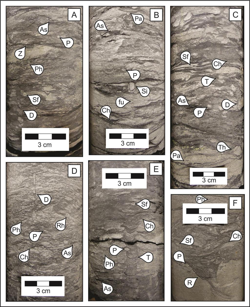
52 37

53 Figure 2.6. Examples of CHF 3. A) Lower very fine- to lower fine-grained bioturbated muddy to silty sandstone. Units show BI 4-5. Trace fossils include Asterosoma (As), Planolites (P), Zoophycos (Z), Phycosiphon (Ph), Schaubcylindrichnus freyi (Sf), and Diplocraterion (D). B) Lower finegrained bioturbated silty sandstone (BI 4-5) with interbedded mudstone and laminated sandstone. Trace fossils include Palaeophycus (Pa), Asterosoma (As), Planolites (P), Siphonichnus (Si), Chondrites (Ch) and fugichnia (fu). C) Lower fine-grained bioturbated muddy to silty sandstone (BI 4-5) with interbedded mudstone and laminated sandstone. Trace fossils include Schaubcylindrichnus freyi (Sf), Chondrites (Ch), Teichichnus (T), Asterosoma (As), Planolites (P), Diplocraterion (D), Palaeophycus (Pa), and Thalassinoides (Th). D) Lower fine-grained bioturbated muddy to silty sandstone (BI 5). Trace fossils include Diplocraterion (D), Phycosiphon (Ph), Planolites (P), Rhizocorallium (Rh), Chondrites (Ch), and Asterosoma (As). E) Lower very fine-grained bioturbated muddy to silty sandstone (BI 4-5). Trace fossils include Schaubcylindrichnus freyi (Sf), Chondrites (Ch), Phycosiphon (Ph), Planolites (P), Teichichnus (T), and Asterosoma (As). F) Lower finegrained bioturbated silty sandstone (BI 4-5) with interbedded mudstone and laminated sandstone. Trace fossils include Phycosiphon (Ph), Schaubcylindrichnus freyi (Sf), Chondrites (Ch), Planolites (P), and Rosselia (Ro) CHF 4: Interbedded mudstone and silty sandstone CHF 4 consists of mudstones interbedded with lower very fined-grained silty sandstone beds (Figure 2.7). The mudstone to silty sandstone ratios range between 3:1 and 1:2, respectively. The discrete mudstone beds range in thickness from centimetres to decimeters, and are generally unburrowed, apparently structureless, and locally carbonaceous. These beds are undulatory in morphology, laterally continuous, and may be sharp-based or draped over silty sandstone beds. The silty sandstone beds are cmscale in thickness and exhibit planar to wavy parallel laminae, current ripples, or rare HCS. Some laminated sandstones also show normal grading. Bioturbation intensities range from low to moderate (BI 2-4) and occur only locally in some mudstone beds. The trace fossils are reduced in size compared to those observed in other HFs (i.e., comparatively diminutive) and include, in order of decreasing abundance, Phycosiphon, Chondrites, Planolites, Schaubcylindrichnus freyi, Thalassinoides, Skolithos, Palaeophycus, and Diplocraterion. In CHF 4, the sharp-based mudstone beds suggest rapid deposition, possibly by hyperpycnal plumes, whereas the mud drapes are regarded to reflect suspension 38

54 settling of mud from hypopycnal plumes. The presence of either mud bed type suggests proximity to a fluvial source. The current ripples observed in some silty sandstone beds reflect unidirectional flow, whereas the wavy parallel laminae reflect oscillatory flow, suggesting a mixed wave- and fluvial-influenced environment. The silty, laminated (locally HCS-bearing) sandstone beds with normal grading are interpreted as tempestites. The general lack of bioturbation indicates stressed conditions, such as overall high-energy conditions, and/or rapid sedimentation rates. The diminution of trace-fossil sizes suggests chemical stresses, such as salinity fluctuations associated with fluvial influence. CHF 4 is interpreted to have been deposited in a storm-influenced, proximal prodelta to distal delta-front. In this study, deposits from both proximal prodelta and distal delta-front represent the same CHF because they have similar average hydraulic conductivities. 39

55 40

56 Figure 2.7. Examples of CHF 4. A) Interbedded mudstone and silty sandstone. The mudstone beds are structureless, and the sandstone beds exhibit planar parallel laminae. Units show BI 0-2. The trace -fossil suite includes Thalassinoides (Th), Chondrites (Ch), Diplocraterion (D), Planolites (P), and Phycosiphon (Ph). B) Apparently structureless mudstone, interbedded with planar parallel to wavy laminated silty sandstone. Bioturbation intensities range from BI 0-3. Trace fossils include fugichnia (fu), Planolites (P), Phycosiphon (Ph), Chondrites (Ch), and possible Skolithos (Sk?). C) Interlaminated mudstone and silty sandstone with bentonite cementation. Units show BI 0-1. Trace fossils are diminutive and include Planolites (P), Chondrites (Ch), and Phycosiphon (Ph). D) Apparently structureless mudstone interbedded with laminated silty sandstone CHF 5: Sandstone with mudstone interlaminae/interbeds CHF 5 comprises upper fine- to lower medium-grained sandstones with less than 10% discrete mudstone interlaminae, interbeds, and rare rip-up clasts (Figure 2.8). The sandstone beds vary from cm- to dm-scale in thickness. Beds vary from apparently structureless to stacked successions bearing HCS or horizontal to low-angle (10-15 ) planar parallel laminae. Bioturbation intensities are low or absent in the sandstone beds (BI 0-1), with a trace-fossil suite that includes (in order of decreasing abundance) Phycosiphon, Schaubcylindrichnus freyi, Schaubcylindrichnus coronus, Diplocraterion, Rosselia, Asterosoma, Zoophycos, Palaeophycus, Skolithos, fugichnia, and rare Ophiomorpha. Discrete mudstone laminae and beds are undulatory and laterally continuous across the width of the core. These units range from millimetres to centimetres in thickness and tend to be sharp based. Bioturbation intensities in the mudstone range from absent to moderate (BI 0-3), with Chondrites, Planolites, Teichichnus, Thalassinoides, Palaeophycus, and Bergaueria comprising the suite. The massive to laminated sandstone beds suggest high-energy deposition and elevated sedimentation rates. The amalgamated laminated sandstone beds were likely deposited by successive storm events that scoured into underlying storm beds. The low bioturbation intensities, the presence of escape structures, and rip-up clasts are likewise consistent with high depositional energy. The unbioturbated, sharp-based mudstone interlaminae are attributed to fluvially sourced mud deposition, probably from flocculation associated with hypopycnal plumes. CHF 5 is interpreted to reflect deposition in a storm-dominated distal delta-front. 41

57 Figure 2.8. Examples of CHF 5. A) Lower medium-grained sandstone with low-angle planar parallel laminae and possible cryptic bioturbation. B) Wavy laminated, upper fine-grained sandstone. Unit shows BI 0-1. Trace fossils include Chondrites (Ch) and Zoophycos (Z). C) Lower mediumgrained sandstone with HCS. The rip-up clast (rc) layer in the photo is likely composed of eroded and transported fragments of Rosselia, Palaeophycus, or Asterosoma. D) Lower medium-grained sandstone. The trace-fossil suite includes Rosselia (Ro), possible Asterosoma (As?), Chondrites (Ch), Skolithos (Sk), Planolites (P), and Phycosiphon (Ph) Stratigraphic Cross Sections In addition to permeability data, AccuMap also archives geophysical well logs. For stratigraphic correlation, gamma-ray logs are particularly useful (Slatt, 2006). Gamma radiation is naturally emitted by uranium, thorium and potassium. In general, an increase in gamma radiation indicates the presence of shale or mudstone, because 42

58 these rock types are composed of clay minerals, potassium feldspar, and organic material (Slatt, 2006). Coarser-grained sedimentary rocks, such as sandstones, contain less of the materials that emit gamma radiation, with the exception of arkose, which is rich in potassium feldspar. Correspondingly, most sandstones are characterized by a decrease in gamma radiation in the gamma-ray logs (Slatt, 2006). Using the interpreted core logs (logged for CHFs) and gamma-ray logs, stratigraphic cross sections along A-A and B-B were constructed (see inset maps in Figure 2.9 and Figure 2.10). Cross-section A-A is oriented along the regional depositional dip and trends NE to SW for a total length of km (Figure 2.9). Crosssection B-B is strike-oriented and trends NW to SE for a total length of km (Figure 2.10). First, discrete CHFs were correlated over cross sections A-A and B-B using 13 wells and their corresponding gamma-ray logs. The interval used in the construction of the cross sections corresponds to the top and bottom of the Viking Formation. The Viking Formation overlies marine shale of the Joli Fou Formation and is capped by marine shale of the Westgate Formation. These low-permeability shale intervals are also indicated on the gamma-ray logs (Appendix B). Consequently, HF 1 is extended above and below the logged interval for both the stratigraphic and hydrogeological cross sections. The cross sections were constructed based on depositional stratigraphy using a laterally continuous bentonite bed as the datum. The bentonite bed is apparent in both the logged cores and on the geophysical well logs. On the geophysical logs, the bentonite is indicated by an increase in the gamma-ray signature. The CHFs, however, do not reflect genetically related facies deposited in the changing environment, and therefore cannot be used for the interpretation of depositional environments. Instead, the depositional stratigraphic sections of A-A and B-B show the distribution and architecture of the different hydrofacies as they were deposited. 43

59 Figure 2.9. Stratigraphic cross-section A-A constructed using composite hydrofacies (CHF). 44

60 Figure Stratigraphic cross-section B-B constructed using composite hydrofacies (CHF). 45

61 Chapter 3. Statistical Modeling of Biogenically Enhanced Permeability in Tight Reservoir Rock This chapter has been published as Hsieh, A.I., Allen, D.M., and MacEachern, J.A., Statistical modelling of biogenically enhanced permeability in tight reservoir rock. Journal of Marine and Petroleum Geology 65, Introduction The storage capacity and productivity of a reservoir are determined by its porosity and permeability. Permeability is also an important factor that controls reservoir response during enhanced recovery. Correspondingly, understanding and projecting variations in porosity and permeability within a reservoir are vital to maximizing the acquisition of the resource. Recently, there has been considerable interest in recovering hydrocarbons from marginal (generally lower-quality) reservoirs using horizontal drilling techniques and fracturing, particularly in areas prone to light oil. The so-called Tight Oil play of the Viking Formation in east-central Alberta and west-central Saskatchewan is one example. Tight reservoirs are characterized by permeabilities that range from md (Spencer, 1989; Holditch, 2006; Clarkson and Pedersen, 2010). In such reservoirs, subtle changes in the distribution of sedimentary media, such as are generated by bioturbation, can greatly affect the porosity and permeability distribution of the facies (e.g., Gingras et al., 1999; Pemberton and Gingras, 2005; Gingras et al., 2007; Tonkin et al., 2010; Baniak et al., 2012). 46 Bioturbation remains an under-appreciated mechanism by which porosity and permeability of a sedimentary facies are modified (cf. Pemberton and Gingras, 2005). Even when considered, bioturbation is generally perceived to be detrimental to bulk permeability, through reduction of primary grain sorting, homogenization of the sediment, and introduction of 46

62 mud through linings, biogenic deposits, and feces (Qi, 1998; Dornbos et al., 2000; Qi et al., 2000; McDowell et al., 2001; Pemberton and Gingras, 2005; Tonkin et al., 2010; Lemiski et al., 2011; La Croix et al., 2013). Recent studies have shown, however, that several ichnogenera and their associated biogenic fabrics are capable of increasing a reservoir rock s porosity and permeability (Gingras et al., 2004; Pemberton and Gingras, 2005; Hovikoski et al., 2007; Volkenborn et al., 2007; Cunningham et al., 2009; Tonkin et al., 2010; Lemiski et al., 2011; Gingras et al., 2012; La Croix et al., 2013; Knaust, 2014). Ichnogenera that form branching burrow networks can create flow pathways in otherwise less permeable units where the burrow fills consist of coarser grains and better-connected intergranular pore space relative to the surrounding matrix (Figure 3.1; Gingras et al., 2004; Pemberton and Gingras, 2005; Lemiski et al., 2011; Gingras et al., 2012; La Croix et al., 2013). Additionally, burrows are capable of increasing vertical permeability in laminated sedimentary rocks, where horizontal permeability otherwise tends to dominate (Gingras et al., 2012). Burrow fills also may undergo diagenetic changes that may lead to higher permeability than that of the surrounding matrix (Pemberton and Gingras, 2005; Tonkin et al., 2010; Gingras et al., 2012). 47

63 Figure 3.1. Sand-filled trace fossils such as Thalassinoides (Th) and Planolites (Pl) create potential flow paths in an otherwise low-permeability unit. Mud-filled traces are dominated by Phycosiphon (Ph). Despite this, permeability across unfractured sedimentary reservoirs is commonly assessed solely on the basis of grain size (e.g. lithostratigraphic units). By contrast, this paper proposes the use of hydrofacies (HF) in reservoir characterization. A hydrofacies is defined herein as a recurring sedimentary facies possessing a distinct permeability grade generated by a combination of sedimentological and ichnological characteristics. Such a hydrofacies takes into account the lithology, textural characteristics, physical and biogenic fabric, the presence and distribution of trace fossils, and the expression of burrow fill(s), all of which serve to affect permeable flow pathways (vertically and laterally) in heterolithic facies. The Markov chain approach proposed in this paper is used to compare vertical transitions in permeability within a borehole with transitions in a) grain size, and b) hydrofacies at the bed to bedset scale, in order to determine which variable best reflects the observed permeability variations. 48

64 3.2. Geologic Setting The Lower Cretaceous (Upper Albian) Viking Formation is a prolific oil- and gasproducing interval that was deposited in the Western Canada foreland basin during a period of active tectonism and eustatic sea level fluctuations. During Viking deposition, a shallow epicontinental seaway extended from the Arctic Ocean to the Gulf of Mexico (Figure 3.2; Williams and Stelck, 1975; Caldwell, 1984; Walker, 1990; Reinson et al., 1994), into which was deposited a complex succession of siliciclastics, dominated by mudstones, heterolithic bedsets of sandstone and shale, and sandstones, with minor conglomerates. Figure 3.2. Map showing the major hydrocarbon-producing fields of the Viking Formation in Alberta (MacEachern et al., 1999). The Viking Formation stratigraphically overlies the Joli Fou Formation and underlies the Westgate Formation (Figure 3.3; Stelck, 1958). It is generally regarded to be roughly equivalent to the Paddy Member of the Peace River Formation of northwestern Alberta (Leckie et al., 1990), and the Bow Island Formation of southern Alberta and southwestern Saskatchewan 49

65 (Figure 3.3; Stelck and Koke, 1987; Raychaudhuri and Pemberton, 1992). Whereas the Viking sediments only range from 15 to 30 m in thickness, they are discontinuity bound and depositionally complex, resulting in sedimentary successions, facies, and geometries that are challenging to characterize and correlate (e.g. Pattison, 1991; Reinson et al., 1994; Walker, 1995; Burton and Walker, 1999). Figure 3.3. Stratigraphic correlation diagram of the Viking Formation in central Alberta showing the overlying Westgate Formation, underlying Joli Fou Formation, as well as its stratigraphic equivalents, the Paddy Member and Bow Island Formation (MacEachern et al., 1999). The Late Albian (Lower Cretaceous) Viking Formation comprises a siliciclastic succession consisting of interstratified mudstones, sandstones and rare conglomerates, mainly reflecting shoreface, delta and estuarine valley deposits. These clastic sediments were supplied from the rising Cordillera in the west and reflect northward and eastward progradation of environments into the Alberta foreland basin. The Viking Formation overlies marine shale of the Joli Fou Formation and is capped by marine shale of the Westgate Formation (Figure 3.3). The stratigraphic relationships were addressed by the work of Stelck (1958), Glaister (1959), 50

66 McGookey et al. (1972), Weimer (1984), Cobban and Kennedy (1989), Stelck and Leckie (1990), Bloch et al. (1993), Caldwell et al. (1993), and Obradovich (1993). The Viking Formation is internally complex stratigraphically, and characterized by numerous internal discontinuities. Beaumont (1984), Boreen and Walker (1991), Pattison (1991), Posamentier and Chamberlain (1993), Reinson et al. (1994), Walker (1995), Burton and Walker (1999), and MacEachern et al. (1999), among others, have attempted to provide allostratigraphic and sequence stratigraphic assessments of the Viking, with varying levels of success. Viking Formation discontinuities have been linked to the global changes of sea level outlined in Kauffman (1977), Vail et al. (1977), Weimer (1984), and Haq et al. (1987). A cored interval of the Viking Formation from the Verger Field was selected for this study because it exhibits stacked parasequences characterized by the interstratification of impermeable and permeable beds with variable but locally pervasive bioturbation Geostatistics In this study, the transition probability method is used to model bioturbated, heterogeneous sedimentary media. The transition probability method is a modified form of indicator kriging that assumes the type of sediment that will be deposited in a stratigraphic succession depends solely upon what is currently being deposited in the present environment and not on the rock types deposited in past environments (Jones et al., 2002). For example, in a prograding shoreface environment, one would expect to find a gradual upward-coarsening succession of facies. If the rock type observed is fine-grained parallel laminated sandstone of the middle shoreface, the next unit to be deposited is more likely to be coarser-grained crossstratified sandstone of the upper shoreface, regardless of what rock type was deposited before the fine-grained parallel laminated sandstone. In terms of spatial distributions, the probability of the occurrence of a class is dependent on the nearest occurrence of another class over a specified lag interval. The probability of class 1 passing into class 2 can be defined by: p 12 h Φ = Pr{(class 2 occurs at x + h Φ ) (class 1 occurs at x)} (3.1) where h Φ represents the lag distance in the direction Φ (Carle, 1999). 51

67 The spatial correlation among different sedimentary facies can be calculated using a Markov chain analysis; a mathematical model that transitions from one state to another between a fixed number of possible discrete states (Carle, 1999). For example, a succession of sedimentary facies may be characterized by a preferred tendency for sediment A to be deposited after sediment B, but not sediment C; therefore, the spatial occurrence of sediment A may be dependent on the pre-existence of sediment B but independent of sediment C (Li et al., 2005). Additionally, if sediments A, B, and C tend to be deposited upwards as a sequence ABC, this asymmetric relationship also can be characterized using Markov chain analysis (Li et al., 2005). The Markov chain is described as follows: There is a set of classes, S = {s 1, s 2,, s r }, which pass sequentially from one to another in steps. The probability of class s 1 moving to class s 2 is represented by p 12, otherwise known as the transitional probability from s 1 to s 2. If the transition remains in the same class s 1, it is denoted by the probability p 11 (Grinstead and Snell, 1997). For example, Carle (1999) assessed the transition probabilities down a well log using an embedded analysis of the Markov chain with respect to a matrix of vertical transitions from one discrete sedimentary facies to another. In that study, an embedded Markov chain analysis of a vertical succession was defined by three facies (A, B, and C) according to the following steps (Carle, 1999): 1. Disregard the lag or spatial dependency and relative thicknesses of the beds. 2. Log the embedded occurrences of A, B, and C down the borehole (e.g. ABCABACABCABABC). 3. Count the number of transitions from one state to another in a transition count matrix. A B C A B 2-3 C Self-transitions (e.g. from A to A) are unobservable in single or stacked beds, and are therefore null in the transition matrix. 52

68 4. Divide each transition count by the sum of the row, in order to find the embedded transition probabilities. A B C A B C This final matrix shows the transition probabilities for each combination of units. The Markov transition probability approach is generally useful for stratigraphically confined systems. As is clear from Walther s Law, genetic and predictable relationships exist for facies successions that occur between stratigraphic breaks, which are absent in facies separated by such breaks. Markov transition probability can be used to demonstrate the lack of correlatibility of facies across such stratigraphic breaks (Weissmann, 2005). Another advantage of using Markov chain models is that the approach assumes stratigraphic stationarity (statistical homogeneity; i.e. the mean and standard deviation do not change over time or space) across the modeled reservoir (Weissmann, 2005). In other words, by dividing the core into facies, the proportions and geometries of different facies within the environment are maintained. In a transgressive marine environment, for example, the proportion of fine-grained facies is higher than coarse-grained facies across the environment, and the probability of fine-grained facies being deposited is likewise greater. This ensures that a facies represented in the model is not a result of random variables, but rather is reflective of the character of the depositional conditions. Furthermore, the distribution of facies within the stratigraphic unit theoretically can be simulated, resulting in a quantifiable conceptual model that facilitates the interpretation of the reservoir s heterogeneity (Weissmann, 2005) Methodology Logging Well W4 in the Verger Field contains core through the Viking Formation, and was selected for this study because it exhibits the interlayering of impermeable and permeable beds (e.g. mudstones and sandstones) that are thoroughly bioturbated in certain sections. All of 53

69 the physical and biogenic features observed in the core, including lithology, grain size, bioturbation index (BI) and ichnological suites, were logged from the base to the top of the well using AppleCORE, a core-logging program that allows the user to record descriptive geological data and convert the data into a strip log (Figure 3.6) Permeability Data The permeability data for the well were obtained from AccuMap, an oil and gas mapping, data management and analysis software for companies operating in the Western Canadian Sedimentary Basin and Frontier areas (AccuMap IHS; accessed 06 February, 2013). The AccuMap data for well W4 include 44 horizontal permeability (k max ) values that were measured at discrete locations over the length of the core. Each k max value was measured using both plug and full diameter samples from the core. At the bed/bedset scale, an average k max value was calculated from the raw permeability data to represent each HF as described below. For the transition probability analysis, the k max values were classed by increasing magnitudes in logarithmic scale (0.01, 0.1, 1, 10, and 100 md) to enable comparison firstly between permeability and grain size, and secondly between permeability and HF Hydrofacies and Parameter Class Divisions Hydrofacies (HF) were qualitatively defined at the bed/bedset scale based on distinct sedimentary, ichnological, and potential permeability attributes. The average grain sizes observed in the core were divided according to the Wentworth (1922) grain-size classification scale: clay, silt, lower fine-grained sand, upper fine-grained sand, and lower medium-grained sand. Bioturbation index (BI) reflects grades of bioturbation intensity, and were assigned values from 0 to 6, with 0 being unburrowed, and 6 being the most intensely burrowed (Figure 3.4; Reineck, 1963; Taylor and Goldring, 1993; Taylor et al., 2003). BI values of 6 (complete bioturbation) were not observed in the cored interval. 54

70 Figure 3.4. Schematic diagram of the bioturbation index (BI), modified from Reineck (1963), Taylor and Goldring (1993) and Taylor et al. (2003) by MacEachern and Bann (2008). Bioturbation grades correspond to: BI 0 = 0% bioturbation; BI 1 = 1-4% bioturbation; BI 2 = 5-30% bioturbation; BI 3 = 31-60% bioturbation; BI 4 = 61-90% bioturbation; BI 5 = 91-99% bioturbation; and BI 6 = 100%. 55

71 Transition Probability Analysis The probabilities of each class transitioning to another were calculated using the Transition Probability Geostatistical Software (T-PROGS), developed by Carle (1999) within the Groundwater Modelling Software (GMS version 6.0, Copyright 2013 Aquaveo). The transition probability matrices for grain size and HF were compared to that of k max. In a transition probability matrix, the self-transition curves start at a probability of one or 100% and decrease with increasing lag distances, whereas the off-diagonal curves start at a probability of zero (0%) and increase with lag distance (Carle, 1999). In both cases, the curves eventually reach a limit, and the probability corresponding to the limit of the curve is called the sill, and represents the mean volumetric proportion of the material. The lag distance at which the curve reaches its limit is known as the range. The lag distance at which a tangent line from the early part of a self-transition curve intersects the horizontal (lag distance) axis represents the mean lens length, or thickness, for the material. The slope of this tangent line represents the transition rate (Figure 3.5). Figure 3.5. Example of a Markov chain transiogram. The transition probability value at which the curve reaches its limit is the sill. The lag distance at which the Markov chain reaches the sill is the range. The slope of the tangent line is the transition rate of the material, and the point at which the tangent line intersects the x-axis is the mean les length of the material. 56

72 3.5. Results and Discussion Hydrofacies Five hydrofacies were identified at the bed/bedset scale in the studied core (Table 3.1): bioturbated/non-bioturbated mudstone; bioturbated silty mudstone; bioturbated muddy sandstone; bioturbated sandstone; and sandstone. For the logged core, only plug permeability data were available for HF 4 and 5, and only full-diameter core permeability data were available for HF 2 and 3. The plug and full-diameter core analyses capture permeability at different scales. The plug permeability represents k at the bed scale, whereas full-diameter permeability analyses capture bulk permeability. In heterogeneous units, for example, the plug permeability may be biased towards coarser-grained more permeable units, while full diameter analyses capture the permeability of both coarse- and fine-grained units and is more representative of the overall permeability. Due to the paucity of data, however, the plug and full diameter permeability measurements are assumed to be equivalent. Additionally, because the plug samples only measure k max in the horizontal direction, the horizontal k max measured in the full diameter samples were used instead of vertical k. The average permeability (k ave ) is calculated for HF 2, 3, and 5. For HF 4, only one permeability measurement was available, so that value (k max ) is assumed to be representative for all HF 4 at the bed/bedset scale. Permeability was not measured for any of the mudstone hydrofacies (HF 1); therefore, the geometric mean (geomean) of the range of mudstone permeabilities measured in other studies was used (e.g. Mesri and Olson, 1971; Long, 1979; Long and Hobbs, 1979; Nagaraj et al., 1994; Dewhurst et al., 1998, 1999; Yang and Aplin, 2007, 2010). Table 3.1 reports the average or representative k values for each HF. 57

73 Table 3.1. Bed/bedset scale hydrofacies descriptions. The calculated k ave (md) or representative k ave based on previous studies for each HF are also reported. Hydrofacies Lithology Grain Size Sedimentary Structures BI Trace Fossils (in approximate order of decreasing abundance) 1 Apparently structureless mudstone 2 Bioturbated silty mudstone 3 Bioturbated muddy sandstone 4 Bioturbated sandstone Mudstone Clay Apparently structureless, sharp-based mudstone Mudstone with moderate proportions of interstitial silt and sand Sandstone with moderate proportions of interstitial silt and clay Sandstone Lower to upper silt Lower fineto upper fine-grained sand Lower fineto upper fine-grained sand 5 Sandstone Sandstone Lower fineto upper fine-grained sand a Calculated geometric mean of values from the literature b Only one value available for the core No sedimentary structures observed No sedimentary structures observed Apparently low (BI 0-1) or high (BI 4-5) if bioturbation is present and observable Rare Chondrites and Planolites 4-5 Phycosiphon, Chondrites, Helminthopsis, Planolites, Asterosoma, Schaubcylindrichnus, Thalassinoides, Teichichnus, Zoophycos, Diplocraterion, with rare Rosselia and fugichnia k ave (md) 1.31E-04a Phycosiphon, Chondrites, Helminthopsis, Planolites, Asterosoma, Teichichnus, Schaubcylindrichnus, Zoophycos, Thalassinoides, Palaeophycus, Diplocraterion, Skolithos, Ophiomorpha, Rosselia, Rhizocorallium and fugichnia 1.24 Apparently structureless 4-5 Phycosiphon, Asterosoma, and fugichnia HCS or horizontal to lowangle (5 ) planar parallel laminated or wave ripple laminated, sharp-based 0 Not observed 5.03b

74 Figure 3.6. log of PCP Verger W4. 59

75 HF 1 encompasses apparently structureless, sharp-based mudstones (Figure 3.7). Bioturbation may appear absent (BI 0-1) owing to a homogeneously muddy matrix, but where interstitial silt and sand contents are slightly higher or burrows reflect sand or silt segregation from the matrix, bioturbation intensities may range from 4-5. Trace fossils in HF 1 include rare Chondrites and Planolites. The k ave calculated from previous work is 1.31E-04 md (cf. Mesri and Olson, 1971; Long, 1979; Long and Hobbs, 1979; Nagaraj et al., 1994; Dewhurst et al., 1998, 1999; Yang and Aplin, 2007, 2010). HF 2 corresponds to bioturbated silty mudstone with moderate proportions of interstitial silt and sand (Figure 3.7). Primary stratification is not preserved. Bioturbation intensities are high (BI 4-5) with a diverse trace-fossil suite consisting of Phycosiphon, Chondrites, Helminthopsis, Planolites, Asterosoma, Schaubcylindrichnus, Thalassinoides, Teichichnus, Zoophycos, Diplocraterion, with rare Rosselia and fugichnia, in order of approximate decreasing abundance. The k ave value for HF 2 is 0.35 md. HF 3 is characterized by bioturbated muddy sandstones with moderate proportions of interstitial silt and clay (Figure 3.7). No primary sedimentary structures are preserved in HF 3 due to the high bioturbation intensities (BI 3-5). The diverse trace-fossil suite, in order of approximate decreasing abundance, comprises Phycosiphon, Chondrites, Helminthopsis, Planolites, Asterosoma, Teichichnus, Schaubcylindrichnus, Zoophycos, Thalassinoides, Palaeophycus, Diplocraterion, Skolithos, Ophiomorpha, Rosselia, Rhizocorallium and fugichnia. The k ave value for HF 3 is 1.24 md. HF 4 consists of sandstones with rare preserved primary sedimentary structures due to bioturbation (Figure 3.7). Bioturbation intensities range from BI 4-5, and the trace-fossil suite includes isolated Phycosiphon, Asterosoma, and fugichnia. The representative k value for HF 4 is 5.03 md. HF 5 is composed of unburrowed (BI 0), well-sorted sandstones that are hummocky cross-stratified, horizontal to low-angle (5 ) planar parallel laminated, or wave-ripple laminated (Figure 3.7). The k ave value for HF 5 is 4.20 md. 60

76 61

77 Figure 3.7. Examples of hydrofacies. A) Hydrofacies (HF) 3, 4, and 5 with Phycosiphon (Ph), Planolites (P), Scolicia (Sc), Asterosoma (As), and Schaubcylindrichnus (Sch). HF 5 exhibits planar parallel laminae. B) HF 2 with Chondrites (Ch), Asterosoma (As), and Phycosiphon (Ph) interbedded with laminated HF 4 containing Asterosoma (As) and fugichnia (fu). C) Wave ripple laminated HF 5 overlying HF 3 and HF 1. Trace fossils in HF 3 include Phycosiphon (Ph) and Schaubcylindrichnus (Sch). D) HF 5 and HF 4 interbedded with HF 1. Trace fossils in HF 4 include Asterosoma (As) and Phycosiphon (Ph). Trace fossils in HF 1 include Planolites (P) and Chondrites (Ch) Transition Probability (Markov Chain) Analyses The transition probability matrices are shown in Figure 3.8 for grain size vs. k max and in Figure 3.9 for HF vs. k max. The transitions from class 1 to 2 are read from rows to columns. The dominant control on permeability should have similar transition probability curves as k max. The Markov chains for grain size (Figure 3.8) show similar transition probability trends only in column 1 and column 5. Units with clay-sized grains typically appear structureless, and mud-filled trace fossils dominate the trace-fossil suite observed within these units. Units dominated by lower medium (ml)-grained sandstone typically lack bioturbation, and are structureless or laminated. This suggests that grain size only influences permeability where the rock units are relatively homogeneous, whereas intermediate permeabilities (i.e., md) are controlled by a number of variables captured by the hydrofacies. The k max values were classed for the transition probability analyses to enable comparison of the two approaches. 62

78 Figure 3.8. Vertical transition probability matrix for k max (solid black line) vs. grain size (dashed gray line). fl: lower fine-grained; fu: upper fine-grained; ml: lower medium-grained. The transition probability matrix for HF shows superior correspondence to k max (Figure 3.9). The Markov chains show that transitions from one k max class to another vertically down the well are closely related to transitions from one HF class to another. For example, the matrix shows that for column 2, the probability of k max transitioning to 0.1 md is similar to the probability of a particular HF transitioning to HF 2, which is a silty mudstone containing moderate proportions of interstitial silt and sand and generally high bioturbation intensities (BI 4-5). plug analyses show that HF 2 has a geometric average permeability of 0.35 md, which is consistent with k max class (0.1 md) used in the transition probability analysis. The difference in transition rates between HF and k max implies that their average bed thicknesses are different. The discrepancy between HF 3 and k max, as seen in column 3 of Figure 3.9 suggests that the classification used here for k max (1.0 to < 10 md) may not fully capture the permeability characteristics of HF 3. 63

79 Figure 3.9. Vertical transition probability matrix for k max (solid black line) vs. hydrofacies (dotted gray line). The results of the Markov transition probability were also analyzed for correlation. A correlation of +100% indicates a perfect direct relationship between two variables, and a correlation of -100% indicates a perfect inverse relationship. A correlation of zero indicates a lack of correlation (Davis, 1986). The Markov chains show that the volumetric proportions, as indicated by the sill values of different k max classes, correlate with grain size by 15%, even though it is commonly assumed that grain size and permeability have a high, positive correlation (coarse grain sizes being associated with high permeability). However, permeability correlates with the established hydrofacies by 97%, indicating that variations in permeability down the well are strongly related to variations in the HF. 64

80 3.6. Conclusions The results from the transition probability analyses show that horizontal permeability does not correlate well with conventional grain size classifications alone, suggesting that permeability is controlled by additional factors, such as sedimentary structures, bioturbation, and sedimentary accessories. In the studied core intervals, bioturbation plays an important role in the creation and alteration of permeable flow paths within these fine-grained units by generating sand-filled burrows and destroying primary sedimentary structures. Therefore, in order to show a consistent correlation between rock type and permeability, it is important to characterize the rock on the basis of all of its physical, chemical, biogenic, and hydraulic properties by defining the hydrofacies. These hydrofacies show a clear and quantifiable relationship to permeability in the vertical direction. The results show that in the studied well, grain size only correlates closely to permeability in homogeneous, very coarse- or very fine-grained rock units such as sandstone (HF 5) or mudstone (HF 1). In contrast, the transiograms for HF show similar sill values with kmax, indicating that the two attributes have comparable volumetric proportions within the cored interval. Nevertheless, the difference in transition rates between HF and kmax indicates that their average bed thicknesses are different. The T-PROGS software used for the transition probability calculations limits the geologic data to a maximum of five different classes, which may be insufficient to adequately represent some geologically complex reservoirs. Other limitations to this study include the small number of permeability values for the studied cored interval. Only horizontal kmax values were available for the transition probability analysis. Additionally, permeability measurements are historically only conducted on the coarsestgrained units, despite the fact that these facies types may not be representative of the dominant flow unit in tight reservoirs. The paucity of permeability analyses in muddy or strongly heterolithic bedsets limits the applicability of statistical analyses. Micropermeametry may be used to refine the kave of each HF, as it measures detailed and precise permeability at the centimetre scale. Nonetheless, the approach for defining hydrofacies is directly applicable to all low-permeability reservoirs, wherein grain size may not be the dominant factor but rather only one of many controls on permeability 65

81 distributions. This approach can potentially be used as a conceptual framework for the spatial modeling of permeability in low-permeability reservoirs. 66

82 Chapter 4. Upscaling Permeability for Regional Flow Modeling 4.1. Average Hydraulic Conductivity for Bed to Bedset Scale HFs As discussed in Chapter 2, five discrete and recurring composite hydrofacies (CHFs) were identified in 28 wells of the Viking Formation from the Provost Field. These are composed of varying proportions of five bed/bedset scale hydrofacies (HFs) defined in Chapter 3, but with different geometric average permeabilities as shown in Table 4.1. The average permeability (md) calculated for these bed/bedset scale hydrofacies were converted a to average hydraulic conductivity (K ave in m/s) for flow modeling. Table 4.1. Bed/bedset scale hydrofacies identified in core and the calculated average hydraulic conductivity (K ave ) in m/s or representative K ave based on previous studies for HF 1. K ave values calculated in Chapter 3 are also shown below. HF: bed/bedset Ch. 3 K ave (m/s) K ave (m/s) 1 * Apparently structureless mudstone/siltstone Bioturbated silty mudstone Bioturbated muddy sandstone Bioturbated sandstone Sandstone * The average hydraulic conductivity for HF a was calculated from Mesri and Olson (1971), Long (1979), Long and Hobbs (1979), Nagaraj et al. (1994), Dewhurst et al. (1998, 1999), and Yang and Aplin (2007, 2010). a 1 Darcy equals m/day under hydrostatic pressure of 0.1 bar/m at a temperature of 20ºC (Duggal and Soni, 1996). 67

83 4.2. Hydraulic Conductivity Estimation for Composite HFs The bed/bedset scale HFs are on the order of centimetres thick a scale that is impractical to capture at the reservoir scale. Therefore, upscaling of the permeability is required. To do this, the cores were re-logged according to composite HFs (CHFs, see Chapter 2), and an upscaled equivalent K estimated for each CHF. The equivalent K represents the thickness-weighted sum of K ave of the bed/bedset scale HFs comprising the CHF. The equivalent K values were calculated for each CHF in both the horizontal (K h ) and vertical (K v ) directions using the following expressions for layered media (Freeze and Cherry, 1979; Figure 4.1): Figure 4.1. Upscaling hydraulic conductivity (K) at the bed to bedset scale to a single equivalent hydraulic conductivity in both the vertical (K v ) and horizontal (K h ) directions for a composite hydrofacies using the expressions for layered media (see Equations 4.1 and 4.2). K h = n K ave m b m m=1 (4.1) b K v = b n bm m=1kavem (4.2) 68

84 where m is the particular bed/bedset scale HF, b is the total thickness of the CHF, K avem is the average hydraulic conductivity measured from plug samples for a particular bed/bedset scale HF, and b m is the thickness of individual beds (cf. Freeze and Cherry, 1979). As only horizontal permeability measurements were available from plug samples, it was assumed that the bed from which the plugs were taken are isotropic at the plug scale. Equations 4.1 and 4.2 likewise assume that each layer is isotropic and homogeneous (Freeze and Cherry, 1979) Validation of Equivalent K To test the equivalency of the K h and K v values assigned to the CHF against those of the layered bed/bedset HFs system, a series of steady state, two-dimensional numerical flow models were run. Each block model corresponds to an interval of core that represents a single CHF. The CHF is, in turn, made up of bed/bedset scale HFs. First, for each block model, a horizontal and a vertical flow simulation were run over the width and length of the core, respectively. The models were first run using the K ave for the individual bed/bedset scale HFs that constitute the section of core. Following that, the models were run again over the same section of core, but using a single K h or K v for the CHF. The models were constructed in the modeling software Visual MODFLOW, a three-dimensional, finite-difference, block-centred groundwater flow model (Version , Schlumberger Water Services). For the block models, the x direction represents the diameter of the core (10 cm), and the y direction represents length (vertical height) of the CHF (Figure 4.2). As MODFLOW only accepts integers for defining the model domain, the length and diameter of the cored sections were scaled up by 100. Thus, the resulting dimensions of the models extend 10 m in the x direction, and vary in the y direction depending on the length of the CHF. A 1 x 1 m grid spacing was used. A single model layer of unit thickness in the z direction was used because only the vertical (y direction) and horizontal (x direction) flow were simulated. Thus, the models are essentially twodimensional. 69

85 For horizontal flow simulations, the left and right boundaries were assigned specified head values of 10 m and 9 m (Figure 4.2 A), whereas the top and bottom of the model were no flow boundaries. To generate a flow field for the vertical flow simulations, the top and base of the model were assigned specified head values of 10 m and 9 m, respectively (Figure 4.2 B). Thus, depending on the length of each model, the hydraulic gradient was different b. The left and right margins were assigned as no flow boundaries. No other boundary conditions were applied. Figure Boundary conditions for A) horizontal flow simulations and B) vertical flow simulations. h refers to the assigned hydraulic head. b The hydraulic gradient is defined as the difference in head (here, 10 9 m) divided by the vertical separation (here, the length of the composite HF for vertical flow simulations). 70

86 The only assigned property was hydraulic conductivity, which varies as described below. Other parameter values in Visual MODFLOW are not needed for steady state flow simulations. As mentioned above, for each interval of core, two separate steady state models were run: one at the bed/bedset scale and one at the composite scale (Figure 4.3). 1. First, flow was simulated using the hydraulic conductivities of the individual beds/bedsets that comprise the interval of core. a) A vertical flow field was generated. This vertical flow depends only on the K values of the stacked sequence and the vertical hydraulic gradient. The hydraulic gradient varies according to the height of the core. Each layer (bed) has an isotropic and homogeneous K of magnitude K ave corresponding to the respective HF. b) Next, a horizontal flow field was generated. This horizontal flow depends on the hydraulic conductivities of layers. The hydraulic gradient is uniform for all models, owing to the same core widths. 2. Simulations were then run over the same interval of core at the composite scale using each equivalent hydraulic conductivity that represents the section (K h or K v ). 3. The discharge (Q in m 3 /s) from 1) and 2) were compared to verify that flow through a heterogeneous, bioturbated unit is the same as that through the CHF in each direction. 4. The resulting horizontal and vertical discharges for the composite scale simulations were grouped according to CHF, and average horizontal and vertical discharges (Q) were calculated for each. 5. Average hydraulic conductivity values in the horizontal and vertical direction were then calculated for each of the five CHFs using the average horizontal and vertical discharge (from step 4), according to the following equation: K = Q A dh dl (4.3) where K is the hydraulic conductivity, Q is the discharge, A is the crosssectional area perpendicular to the flow direction, and dh/dl is the hydraulic gradient (Darcy, 1856). This final step was to confirm that any numerical errors did not affect the results. If the calculated K was the same as the equivalent K in the respective direction, then the simulations were considered robust. In addition, the water balance was calculated for each simulation to confirm that mass was conserved in the numerical simulation. Given the very small bed thicknesses 71

87 for some models and/or the low hydraulic conductivities of the muddier units, the solver settings had to be carefully adjusted to assure water balance closure. Figure 4.3. A) Example of a MODFLOW block model of a cored section with hydrofacies logged at the bed/bedset scale. Each colour represents a different hydrofacies. B) Block model of the same cored section with hydrofacies logged at the composite scale. The results of the numerical block modeling showed that for the horizontal flow models, the discharges Q (m 3 /s) for the bed/bedset HF and the CHFs had an average discrepancy of 0.47%, disregarding one outlier value resulting from poor model convergence (Figure 4.4A; Appendix C). For the vertical flow models, the average 72

88 discrepancy is 1.27% (Figure 4.4B; Appendix D), disregarding five outliers. In general, a discrepancy less than 5% is considered acceptable, and simulations that yielded a discrepancy greater than 5% were considered outliers (Anderson and Woessner, 1992). This suggests that both vertical and horizontal flow through heterogeneous, bioturbated media can be simplified using an upscaled equivalent K that represents the variability in permeability at the bed/bedset scale. 73

89 Figure 4.4. Discharge in Q (m 3 /s) for bed/bedset scale and composite scale fluid flow simulations in the A) horizontal and B) vertical directions. The average horizontal hydraulic conductivity (K h ) generally increases from CHF 1 to 5 (Table 4.2). The resulting average K v, however, did not increase consistently. CHF 3, though finer in average grain size than CHF 5, has a higher average K v. CHF 3 is moderately to intensely bioturbated, and some of the bioturbation may serve to generate vertical flow paths, thereby increasing overall vertical conductivity. Also, the 74

90 discrete and laterally continuous mudstone laminae/beds observed across some cored sections of CHF 5 are potentially capable of decreasing vertical conductivity. Table 4.2. Minimum, maximum, and average horizontal (K h ) and vertical (K v ) conductivities for each composite hydrofacies. Composite HF Min K h (m/s) Max K h (m/s) Avg K h (m/s) Min K v (m/s) Max K v (m/s) Avg K v (m/s) Regional Flow Simulations CHF Model Setup A hydrogeological cross section along B-B was constructed to show the presentday geological structures that control fluid migration (Figure 4.5). Section B-B is aligned with the regional hydraulic gradient (as described below). For this cross section, the datum is sea level, and each hydrofacies is correlated above or below the datum according to its present-day position. 75

91 Figure 4.5. Hydrogeological cross-section B-B constructed using Composite Hydrofacies (CHF). 76

92 The regional hydraulic gradient of formation waters was estimated from the regional-scale hydraulic head distribution map for the Viking Formation constructed using approximately 3600 drill stem tests (Figure 4.6; Bachu et al., 2002). The hydraulic heads vary from >800 m in the south and <600 m in the east to <300 m in the southwest (Figure 4.6). Cross-section B-B intersects a trough, and has an estimated hydraulic gradient that trends roughly SE to NW along the regional strike, parallel to the line of section. The estimated SE-NW trending hydraulic gradient is an oversimplification of the actual system. The hydraulic head contours shown in Figure 4.6 indicate that groundwater flow actually converges from SE to NW. This suggests that the direction of formation water flow is not solely controlled by the regional structural dip towards the SW. In addition to topography, the flow of formation waters is driven by other mechanisms, including compaction, tectonic compression, erosional rebound, and buoyancy, several of which may be active in a basin at any given time (Bachu, 1999). In the Viking Formation, the regional extent of underpressuring and the inward flow of formation waters is driven by erosional rebound and gas zones in the deep basin (Bachu et al., 2002). 77

93 Figure 4.6. Contours of hydraulic head in the Viking Formation, showing the locations of cross-sections A-A and B-B. Contour intervals are in metres. The solid black arrow shows the simplified direction of the groundwater flow, and the dotted gray arrows show actual groundwater flow directions (Modified after Bachu et al., 2002). Estimates of the hydraulic head are shown for the ends of each cross section. 78

94 The hydraulic gradient along cross-section B-B was estimated as follows: dh dl m m = 1000 m km km = m/m (4.4) where dh is the difference in hydraulic head from B to B (Figure 4.6) and dl is the length of B-B. Flow is roughly from SE to NW. The hydrogeological cross section was reproduced in Visual MODFLOW by visually transferring the contacts between CHFs (Figure 4.7). The model domain was discretized to 250 x 100 m in the x and z directions, respectively. A single, 1 m model layer in the y direction was used; thus was model was effectively two-dimensional. The hydraulic conductivities assigned to the CHFs in the cross section are the average K v and K h values for each CHF (refer to step 4 in Section 4.3). The actual hydraulic head values at the NW and SE ends of the profile are m and m; however, because the base of the MODFLOW model is at 0 m rather than m below sea level, the specified head boundaries were adjusted to 1 m and 13.5 m, respectively. Thus, the hydraulic gradient remains the same ( / m = 6.3 x 10-4 as in Equation 4.4). It was assumed that only a horizontal gradient exists, because no data for the vertical gradient are available. The specified head values were assigned across the full vertical thickness of each end of the profile. The top and bottom boundaries of the profile were assigned no flow boundaries. These no flow boundary conditions assume that the flow is constrained to the units in the cross section and that there is no transfer of formation water from this sequence to either an overlying or underlying sequence of rocks, which is likely an oversimplification of the actual system locally. The model was run under steady-state conditions, and the water balance calculated. The average fluid flux along the cross section was calculated using the following equation: q = Q A (4.5) 79

95 where q is the flux (m/s), Q 1 is the discharge (m 3 /s), and A is the cross-sectional area (m 2 ) of the profile (Freeze and Cherry, 1979). Q was estimated from the water balance in Visual MODFLOW (flow exiting the model domain from the specified head boundary in the NW), and A is the total thickness of the domain at that same end. 1 Q is a volumetric flow rate for groundwater moving along a hydraulic gradient; Q is not a production rate. 80

96 Figure 4.7. MODFLOW domain for hydrogeological cross-section B-B showing the hydraulic heads (h) at the NW and SE boundaries. 81

97 Additional Simulations Based on Literature K Values Flow was also simulated along the line of section B-B using hydraulic conductivity ranges for the Viking Formation as published in literature (Table 4.3). In general, the hydraulic conductivity and Darcy flux measured by various sources represent an average of fine- to medium-grained sandstones in the Viking Formation. The measurements were taken from both drill stem tests and core analyses. Bekele et al. (2002) measured maximum permeability parallel with bedding using 69,532 core plugs from both sandstone and mudstone samples. BlackPearl Resources Inc. (2012) performed a pumping test in a Viking Fm sandstone unit and obtained regional estimates for such sandstones. Cao et al. (2014) estimated the permeability range based on lowenergy depositional environments such as delta-front, prodelta, tidal flat, or transitional facies between shoreface and offshore facies (e.g., upper offshore regimes). 82

98 Table 4.3. Hydraulic conductivity (K) values of the Viking Formation measured in published literature, including the measurement techniques used as well as the lithology in which the measurements were taken. K (m/s) Technique Lithology Lerand and Thompson (1976) Sandstone Alho et al. (1977) to Fine- to medium-grained sandstone Bachu (1985) a Drill stem test (DST), core analyses Average of Viking sandstone Bachu (1988) DST, core analyses Average of Viking sandstone Bachu (1999) a DST, core analyses Average of Viking sandstone Bekele et al. (2002) to (sandstone) to (shale) plug analyses Sandstone and shale Cenovus FCCL Ltd. (2009) K h= , K v= DST Average of Viking aquifer BlackPearl Resources Inc. (2012) to Regional estimates, pumping test Average of Viking aquifer Matrix Solutions Inc. (2012) to DST, core analyses Average of Viking sandstone Cao et al. (2014) to Estimates of deposits from lowenergy environments such as deltafront, prodelta, tidal flat, or transitional zone between shoreface and offshore deposits a No hydraulic conductivity values were given. However, an estimated Darcy flux (q) in m/s is available. 83

99 Flow simulations were run using the K values reported for each study in Table 4.3. Where there is a range of K, two simulations were run using the lower limit and the upper limit of the given range. For Bekele et al. (2002), CHFs 1-2 were assigned the K for shale, and CHFs 3-5 were assigned the K for sandstone. Again, one simulation was run using the lower limits of Ks for shale and sandstone, and another was run using the upper limits of Ks. For Cenovus FCCL Ltd. (2009), the K h and K v were assigned to the entire section. Darcy flux values were calculated for each model using the same approach described in the previous section (Equation 4.5) and compared with the flux calculated from the simulation using the average equivalent K calculated for the CHFs CHF Simulation Results Groundwater flows from the SE boundary to the NW boundary, based on the distribution of the equipotential contours generated from the model. The simulated flow regime is consistent with the general regional groundwater flow of the Viking Formation (Figure 4.8). The equipotential contours are relatively parallel throughout CHF 1, but deviate through the CHFs with higher hydraulic conductivities (hydrofacies 3, 4, and 5). This deviation in the equipotential contours is expected for flow through a heterogeneous system and reflects the varying hydraulic conductivities across the section. 84

100 Figure 4.8. Equipotential head contour map of cross-section B-B. Contour units are in metres. The zoomed section illustrates the deviation of flow lines in red arrows. The maximum arrow length corresponds to a maximum velocity of m/s, to which all other vectors are scaled. 85