Using Temperature and Dew Point to Aid Forecasting Springtime Radiational Frost and/or Freezing Temperatures in the NWS La Crosse Service Area

Transcription

1 Using Temperature and Dew Point to Aid Forecasting Springtime Radiational Frost and/or Freezing Temperatures in the NWS La Crosse Service Area WFO La Crosse Climatology Series #21 The formation of radiational frost is governed by many factors, all of which interact in varying degrees, making forecasting a frost or freeze a complex problem. One of the questions is, do any of the factors by themselves, or in combination, have predictive value for radiational frost or freeze formation? This study attempts to answer the question, do a couple of the more basic ones, temperature and dew point of the airmass during the afternoon, have predictive value for the following morning s low temperature and the threat of frost or freeze. The data set used for this study consisted of hourly observations from first order National Weather Service (NWS) sites, from the years 1983 to 1994: Rochester MN (RST), La Crosse WI (LSE) and Madison WI (MSN), representing three different positions in the local landscape. Frost is typically a micro-climate phenomenon, with its formation strongly dependant on the local landscape. These sites were chosen as they represent three different landscape positions. The Rochester site is on a broad, flat ridge-top with favorable exposure to wind flow and nocturnal cold air drainage in all directions. The La Crosse site is on an island in the Mississippi River with wind flow restricted by foot bluffs to the east and west. The valley floor location is a sink for nocturnal cold air drainage, but is modified to some degree by the surrounding water. The Madison site is in a broad terrain bowl with favorable wind exposure but is also a sink for nocturnal cold air drainage. The Madison site could be considered a frost pocket due to its topographic position and surrounding landscape. The study concentrated on April 1 to June 15, annually, with the period divided into onehalf month periods: days 1 15 and 16 30/31. April 1 to June 15 is a period of considerable change, mainly due to the increasing hours of daylight and intensity of incoming solar radiation. Average temperatures increase rather rapidly during this period due to the increasing length of daylight and higher sun angle, and the local vegetation changes from generally dormant at the beginning of April to green and actively transpiring by the end of May. From 1983 through 1994, 233 days were selected that showed a favorable synoptic weather pattern for strong nocturnal radiational cooling. April 1 through June 15 is a period of 76 days. For the study period this consisted of 912 individual days. Most of these days would not have had the potential to produce a radiational frost and would not have been considered a potential radiational frost day (night) by a forecaster analyzing the pattern and data. Since this research attempts to provide some insight into elements helpful for forecasting radiational frost formation (nocturnal radiational cooling to the point where frost could form), it was approached from a forecast perspective. 1

2 Radiational frost formation near and after the average last frost dates, when the probability and frequency of occurrence on any one day is actually rather low and decreasing, requires a favorable synoptic pattern. In the La Crosse forecast area, this is the same synoptic pattern required for radiational valley fog formation. A forecaster concerned with late night valley fog formation looks for a larger scale pattern producing generally clear skies and light winds; usually a high pressure system settling over the area from the west, northwest or north. The NOAA US Daily Weather Maps archive was searched for days with this developing or forecast synoptic pattern supportive of strong radiational cooling and the threat of fog or frost. A total of 233 days, with high pressure centered near or over the area, were gleaned from the 912 possible days in the 12 year data set. 47 of these days were in the first half of April, 58 in the second half, 51 in the first half of May, 42 in the second half and 35 in the first half of June. The hourly observations for the 0900 to 0900 LST period surrounding the 0600 LST valid time of the Daily Weather Map and morning low temperature, were extracted for the 233 days. Within these periods, the 233 days were further separated based on the resulting low temperature. Four categories were used: low temperatures of 32 F or less, 33 F to 37 F, 38 F to 42 F and 43 F or higher. These ranges were chosen based on the areal coverage of frost expected to occur at these temperatures. One has to remember that official observations are taken at a shelter height of 4.5 feet above the ground surface. With strong radiational cooling and a generally calm airmass, micro-inversions develop and low temperatures within a few inches of the ground surface can be 10 F, or more, colder than those observed at 4.5 feet. Shelter height low temperatures of 32 F typically result in widespread frost and damage to tender vegetation across the nearby landscape. Shelter height lows of 33 F to 37 F typically result in areas of frost and some damage to tender vegetation. Lows of 38 F to 42 F at 4.5 feet could result in patchy frost. Frost is not expected with low temperatures of 43 F or higher at the shelter height. Within the various categories, afternoon temperatures (T) and dew points (Td) prior to the morning of a potential frost or freeze were analyzed. The degree of warmth and moisture present in the airmass during the afternoon should have a strong influence on how close to 32 F that airmass can radiatively cool during the subsequent overnight hours. A warmer airmass will require more radiational cooling to reach a frost temperature than a cooler one. The dew point is often considered the first guess for the next morning s low temperature: too high of a dew point and fog or excessive dew would form before reaching a frost temperature. Using the temperature and dew point from the afternoon prior to the morning of concern, the assumption was made that minimal or no advection of a different airmass into the area would occur overnight due to light or calm boundary layer winds. 2

3 Temperature and dew point surface observations from 1100 to 1400 LST, the latest a forecaster would have at his or her disposal, were used in the statistical analysis. These were averaged to eliminate noise in the data, especially the dew point which is a difficult parameter to measure. The initial analysis included temperature and dew point individually, but these had limited use in discriminating between low temperatures in the four temperature categories. A stronger signal was seen for predicting the next morning s low temperature in the four categories when temperature and dew point were summed into a single index value. The four hourly values (e.g LST) of temperature and dew point, in Celsius, were averaged into one index value per case day at each site. Figure 1 illustrates some of the change during the spring season and why the study period was broken up into roughly two week periods. The hours of daylight change from around 13 hours during the first half of April to almost 15.5 hours during the first half of June. This means, and is important to the radiational frost problem, that the hours of darkness changes from around 11 hours during the first half of April to a little more than 9.5 hours during the first half of June. The rapidly changing energy balance of the environment causes a rather rapid rise in the average highs and lows through April, May and June. As this occurs, the chances of a radiational frost or freeze decrease rather rapidly during this period. Hours of Day Light Equinox (Mar 21) Apr 8 Apr 23 May 8 Date May 23 Jun 8 Solstice (Jun 21) Day Length LSE Avg min T LSE Avg max T RST Avg min T RST Avg max T MSN Avg min T MSN Avg max T Temperature (F) Figure 1. Change of day length, average highs and lows during the spring season (based on year averages) at Rochester MN (RST), La Crosse WI (LSE) and Madison WI (MSN). Also shown is the hours of daylight, (line with squares) centered on the middle day of each of the study periods. 3

4 11 10 Standard Dev. ( F) Apr 8 Apr 23 May 8 May 23 Jun 8 LSE Std Dev, LSE std Dev, Full Rec RST Std Dev, RST Std Dev, Full Rec MSN Std Dev, MSN Std Dev, Full Rec Figure 2. Same as Fig. 1, except the standard deviation of low temperatures during the spring season, based on (30 year averages) at Rochester MN (RST), La Crosse WI (LSE) and Madison WI (MSN). The average standard deviation for minimum temperatures for the three sites is very near 8 F (Fig. 2). The average last spring frost date, defined as the occurrence of a low temperature of 32 F or colder, at Rochester, La Crosse and Madison are 5/6, 4/18 and 5/9, respectively. The average low temperature at each site on these dates is near 44 F. 32 F is 12 F or 1.5 standard deviations below the climatological average low on these dates. Following the normal distribution curve, the probability of a 32 F or colder low on the average last frost date is 6.67 percent. Since the standard deviation of the low temperature is nearly constant, the probability of reaching a low of 32 F on any particular day decreases as the average low warms through the season. For the set of 233 study dates, the probability of cooling to a low temperature at or below 37 F or 32 F decreases rapidly from early April to late May (Fig. 3). 4

5 Percentage 100% 90% 80% 70% 60% 50% 40% 30% 20% 10% 0% 4/ / / / / 1 15 Half month Periods LSE <= 32 RST <= 32 MSN <= 32 LSE <= 37 RST <= 37 MSN <= 37 Figure 3. The frequency of occurrence for specific low temperatures during the half month periods, given synoptic conditions favorable for strong radiational cooling. Figure 4. The T+Td index vs. next morning low temperature category for April 16 th to 30 th. LSE is grouped on the left, RST center and MSN on the right. The mean and sample size (SS) is plotted for a particular category for a site and time period when the sample size was less than 5. 5

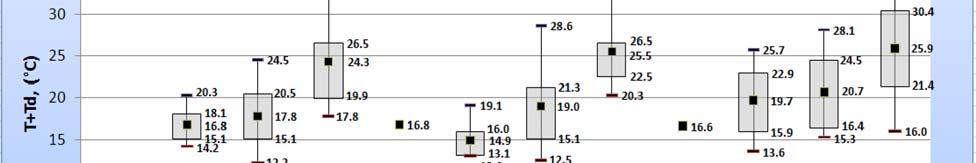
6 Figure 5. Same as Fig. 4, the T+Td index vs. next morning low temperature category for May 1 st to 15 th. Figure 6. Same as Fig. 4, the T+Td index vs. next morning low temperature category for May 16 th to 31 st. 6

7 Figure 7. Same as Fig. 4, The T+Td index vs. next morning low temperature category for June 1 st to 15 th. The April 1-15 period was initially included for analysis of seasonal trends, but it was too early to be concerned with spring frosts given their ease and frequency of occurrence. If a favorable synoptic pattern occurs in early April, there is nearly a 100 percent chance that areas of frost and an 80 percent chance that widespread frost or freezing temperatures would occur (recall Fig. 3). From the trends of the individual sites, it can be seen that the T+Td index does have some value in discriminating between the widespread, areas, patchy or no frost categories (Fig. 4-7, the different heights of the plots for a particular site and time period). This is most apparent in early May, at all three sites (Fig. 5). Seasonal trends can also be seen, with the categorical occurrences weighted toward widespread and areas of frost (<= 32 and categories) in late April (Fig. 4), and toward patchy or no frost (38-42 and >= 43 categories) by early June (Fig. 7). For example, the >= 43 sample sizes in late April (Fig. 4) are too small to calculate meaningful statistics, but by early June (Fig. 7) it is the <=32 and sample sizes that are too small, or non-existent, to calculate meaningful statistics. Differences among the three sites can be seen, but are not quite as visible as the other trends. MSN shows a higher T+Td index for most time periods and categories when compared to LSE. With the MSN observation located at a position in the local landscape where cold air drainage from the surroundings collects, it takes a warmer and more moist airmass to prevent radiational frost from forming when compared to higher or buffered landscape positions like RST and LSE. This susceptibility to lower temperatures and greater frost threat can also be seen in the greater frequency of occurrence of the <= 32 and categories during late May and early June at the MSN site compared to LSE and RST. 7

8 A statistical T-test analysis was done on the data for the different frost categories for each site and each one-half month time period. The test was done to determine the statistical significance of the T+Td index differences. Differences of categorical means of 1.5 o F to 2.0 o F are significantly different with a 90 to 95 percent confidence limit. This means that there is a 90 to 95 percent chance that the groups with averages that are different by 1.5 o F to 2.0 o F are truly different from each other. This is a favorable result and would promise usefulness of this study. However, quite apparent is the overlap of the distributions from category to category for a site within a time period. This diminishes the usefulness of the results of this study. As an example, it is early May and a forecaster is concerned about frost at LSE (which can probably be applied to many of the larger river valley locations). The LST T+Td index is 12 C. A T+Td index of 12 C at La Crosse in early May resides in all four frost categories. It is on the high end of predicting a low of <=32 F (e.g. 80% of this category s cases had lower index values at LST) and on the low end of predicting a low of >=43 F. With an index of 12 C, the F category appears to have the best likelihood of occurrence, falling in the 20 to 80% range. A 12 C index value lies in the tail (whiskers) of the other three frost categories. Given the overlap of the upper or lower tails of the distributions there is no absolute certainty, using only this T+Td index, of knowing which category the next morning s low temperature will verify in. Use these study results only as a guideline when forecasting low temperatures under favorably radiational cooling nights during the mid April through mid June period. The overlap of the box and whisker plots for a site and time period indicate that T and Td trends during the afternoon before a favorable radiational cooling night only partially explain the variability seen in low temperatures the following morning. Scatter plots and correlation coefficients were generated for the afternoon T+Td index and the following morning s low temperature. The scatter plots are the first step in determining the strength of a relationship, or correlation, between two data sets, if there is a relationship at all. Upon visualizing the data, if it appears a linear relationship exists, a correlation coefficient (R) can be calculated. A perfect linear relationship, with all the scatter plot points on a line with some slope (e.g., a given value A results in a specific value B), would have an R value of A plot with points well scattered, or approximating a horizontal line with no slope (e.g., a given value A does not result in any specific value of B) would have an R of R values of less than 0.50 are generally weak relationships, 0.50 to 0.75 are moderate and 0.75 to 1.00 are strong relationships. 8

9 1100 to 1400 LST, Avg T+Td [C] Next Morning Lows (C) 15 Figure 8. Scatter plot of the LST T+Td index vs. the next morning low at RST for May 16 th -31 st. R for this data set is to 1400 LST, Avg Td [ C] Next Morning Lows ( o C) 15 Figure 9. Scatter plot of the LST T+Td index vs. the next morning low at MSN for May 16 th -31 st. R for this data set is Scatter plots were generated for the afternoon 1100 to 1400 LST T, Td and T+Td index vs. the next morning low temperature for each of the five half-month periods at each of the three sites. Of all the analyses, the T+Td index at RST for the second half of May (Fig. 8) shows the strongest linear correlation, and has some predictive value for the next morning s low 9

10 temperature. The R for this relationship is 0.611, or the T+Td index explained about 37% of the variability seen in the next morning s low at RST during the second half of May. The weakest correlation is the LST Td at MSN for the second half of May (Fig. 9). A particular afternoon Td at this site resulted in a wide range morning low temperatures, with the plot approximating a horizontal line. The R for this relationship is 0.016, or Td only explained 0.03% of the variability in the next morning s low at MSN during the second half of May, which is basically no relationship at all. April April May May June By site, All periods Rochester T+Td T Td Madison T+Td T Td La Crosse T+Td T Td All All sites, Sites All periods T+Td T Td Table 1. Correlation coefficient (R) values of afternoon LST average T, Td and T+Td index vs. the next morning low for each site and time period. The T+Td index generally explains more of the variability than T or Td alone, although most are weak or weakly moderate relationships (Table 1). The T+Td index and T have more predictive value at RST and LSE than at MSN. Dew point alone performs better at MSN than at RST and LSE. For all sites combined, the correlations are stronger in May (around 0.50) than in April (around 0.40) and June (around 0.30). However, when all periods and locations are combined, the T+Td index only explained 17.6% of the variability observed in the next morning s low temperature. T explained 13% and Td 5.3%. All of these are weak correlation relationships. Even the better of the three (e.g., the T+Td index) left over 82% of the variability of the next morning s low unexplained. 10

11 Since predicting a radiational frost or freeze is a boundary layer and micro-climate phenomena, even more so than radiational valley fog formation, many factors other than the temperature and moisture content of the airmass can and do impact the eventual next morning s low temperature. 1) The data set was not analyzed for cloud cover. Even a fraction of cloud cover overnight can impact radiational cooling and the next morning s low temperature. 2) The data set was not analyzed for boundary layer wind overnight. Even a very light but steady wind at or just above the surface can keep the boundary layer stirred enough to prevent lows from cooling enough to produce frost. 3) The data set made no distinction or assessment of soil moisture. For a few days after a rainfall, dew points will normally rise some during the evening, with these days being more prone to radiational fog or significant dew formation instead of frost. 4) The stage of vegetation greenness was not analyzed. Once the vegetation greenness increases ( green-up ) and if the landscape is well watered, dew points will rise during the evening, offering some buffer to how much the boundary layer can radiatively cool overnight. One would expect this factor to be most variable during early May, as greenup normally occurs during late April to early May at the study sites. However, early May has some of the stronger T+Td index correlations. 5) The synoptic pattern was not differentiated for the source direction of the surface high pressure system building in. Based on pattern recognition for high fire danger days across the western Great Lakes region, high pressure systems from the north tend to produce more boundary layer drying (lower dew points and afternoon relative humidities) across the study sites than those from the west or northwest. This is a short list of five additional factors one should consider when trying to predict a radiational frost or freeze. With less than 18% of the variability explained by the average temperature and dew point during the afternoon before a favorable radiational cooling night, the results of this study should serve as a guide when attempting to predict the next morning s low temperature and the threat of a frost or freeze. Assessment of at least the five additional factors above should be included in an analysis of a spring time frost or freeze threat. 11