Use Authorization. Signature. Date

Transcription

1 Use Authorization In presenting this thesis in partial fulfillment of the requirements for an advanced degree at Idaho State University, I agree that the Library shall make it freely available for inspection. I further state that permission to download and/or print my thesis for scholarly purposes may be granted by the Dean of the Graduate School, Dean of my academic division, or by the University Librarian. It is understood that any copying or publication of this thesis for financial gain shall not be allowed without my written permission. Signature Date i

2 FLOW MEASURMENT USING CRITICAL FLOW ORIFICES: A Study of Their Limitations and Strengths by Joseph Berrett Maestas A thesis submitted in partial fulfillment of the requirements for the degree of Master of Science in the Department of Mechanical Engineering Idaho State University May 2016 ii

3 Copyright Copyright 2015 Joseph Berrett Maestas iii

4 Committee Approval Page To the Graduate Faculty: The members of the committee appointed to examine the thesis of JOSEPH BERRETT MAESTAS find it satisfactory and recommend that it be accepted. Dr. Richard Schultz, Major Advisor Dr. Ken Bosworth, Committee Member Dr. Bruce Savage, Graduate Faculty Representative iv

5 Acknowledgement Page I would like to show gratitude for all those who made this thesis possible. Thank you Idaho State University for the necessary resources required to produce this thesis. Thank you Dr. Brian Williams for brandishing those resources and helping me in the early stages. Thank you Dr. Ken Bosworth and Dr. Bruce Savage for providing comments and showing professionalism during my thesis defense. A very special thank you to Dr. Richard Schultz for mentoring me and providing expertise and support in the many hours dedicated to this thesis. And lastly, thank you Meranda Maestas for always believing in me, supporting me, and being my rock. v

6 Table of Contents List of Figures... viii List of Tables... ix List of Equations... x Abstract... xi Chapter I: Introduction... 1 Operational Definitions... 3 Significance of the Study... 3 Chapter II: Literature Review... 4 Summary Chapter III: Description of Hardware Chapter IV: Description of Instrumentation Chapter V: Setup and Test Procedure Test Setup Test Procedure Chapter VI: Methodology Zucker Equation Spink Equation Discussion of Differences Between Zucker and Spink Equations Experimentally-Measured Mass Flow Measurement and Calculational Uncertainties Chapter VII: Results Chapter VIII: Conclusions Uncertainties in the Critical Mass Flow Rate Calculated Using Standard Practices Virtues of Using Critical Flow Orifices Future Research Possibilities/Questions for Future Inquiry References Appendices Appendix A: Orifice Area & Downstream Volume Calculation Procedure vi

7 Appendix B: Calibration Process & Leak Test Appendix C: Calculation Examples Appendix D: Test Data Report Appendix E: Diagrams, Graphs, Tables, etc vii

8 List of Figures Figure 1, Orifice Meter... 1 Figure 2, Graph showing the relationship between Cd and t/d (Fig 7 in Ward-Smith, Ref 5) Figure 3, Hardware Identification Figure 4, 1/64-inch Diameter Orifice Plate Figure 5, Orifice Plate Specifications Figure 6, Instrumentation Identification Figure 7, DAQ Output Data Figure 8, Experimental Apparatus Figure 9, DPT wiring to DAQ Figure 10, DAQ wiring Figure 11, DPTs wiring and connections Figure 12, Entrance Line Figure 13, Orifice plate setup Figure 14, Power supply wiring Figure 15, YtSp Trendline Graph Figure 16, 1/16-inch Orifice Plate Test Graphs Figure 17, 1/32-inch Orifice Plate Test Graphs Figure 18, 1/64-inch Regular Orifice Plate Test Graphs Figure 19, 1/64-inch Chamfered Orifice Plate Test Graphs Figure 20, Tank Temperature Graph Figure 21, Pixel Counting Figure 22, Pressure Calibrator Figure 23, Bubble Leak Test viii

9 List of Tables Table 1, Critical Discharge Coefficients... 9 Table 2, Piping, Hardware, and Instrumentation Diagram Table 3, Spink s specification number one Table 4, Uncertainty of Orifice Area and Diameter Table 5, Pressure and Temperature Uncertainties Table 6, Extrapolated YtSp value for the 1/32-inch & 1/64-inch Table 7, Precision Index/Uncertainty Summary Table 8, Average Mass Flow Rates with Uncertainties ix

10 List of Equations Equation 1, Mach Number Equation 2, Speed of Sound Equation 3, Mass Flow Rate Equation 4, Ideal Gas Equation 5, Ideal Mass Flow Rate Equation 6, Zucker's Critical Mass Flow Rate Equation 7, Zucker's Critical Mass Flow Rate with Discharge Coefficient Equation 8, Zucker's Critical Mass Flow Rate Simplified Equation 9, Spink's Critical Mass Flow Rate Equation 10, Spink's YtSp Equation 11, Area of a Circle Equation 12, Area of a Circle Rearranged Equation 13, Mass Equation 14, Mass using Ideal Gas Equation 15, Mass Rate Equation 16, Mass Flow Rate for Constant Volume Equation 17, Benedict-Webb-Rubin Equation 18, Taylor Series Expansion Tailored for Eq Equation 19, Taylor Series Expansion Tailored for Eq Equation 20, Taylor Series Expansion Tailored for Eq x

11 Abstract An experiment and analytical study were perfomed to determine the feasibility of building critical flow orifices for measuring mass flow rate using readily available machine tools (drill press and off-the-shelf drill bits), to determine whether an acceptable mass flow rate measurement could be achieved using standard analytical techniques, and to provide the uncertainties on the orifices, measurements, and instruments. Four sharp edge circular orifice plates with the following diameter hole sizes: 1/16-inch, 1/32-inch, 1/64-inch, and 1/64-inch with an exit chamfer were constructed and used as the basis for both the experiment and the calculations. The work accomplished to both construct the critical flow orifices, assemble the experimental hardware and instrumentation, and conduct the experiments demonstrated that the effort required to use critical flow orifices is straightforward and relatively inexpensive. Certainly construction of critical flow orifices is considerably more straightforward than the design and construction of a critical flow venturi or nozzle and the turnaround time and operational flexibility is overwhelmingly favorable to using critical flow orifices Therefore, on this basis, the overall evidence for using critical flow orifices is very favorable. Measured mass flow rates were obtained using a collection tank downstream of the orifices. Instrumentation such as differential pressure transducers and thermocouples along with a data acquisition system recorded both upstream and downstream conditions of the installed orifice plate. This data were used for both calculating and measuring the mass flow rate. Unfortunately the measured flow rates had unacceptably large uncertainties and therefore only provided qualitative data. xi

12 Based on the calculational uncertainties alone, which in general ranged from 1.5% to 2.9% for the Zucker equation, dependent on the size of the orifice, the results of this study show that critical flow orifices, which have the significant advantage of being simple to construct and install, offer a practical method for obtaining mass flow rates with a reasonably low uncertainty. xii

13 Chapter I: Introduction There are many methods or devices used for the purpose of metering flow. These devices are designed and installed to measure the flow rate with measurement uncertainties explicitly defined in national standards. A common device known as an orifice meter, Figure 1, consists of a housing, orifice plate, and pressure taps. The orifice plate is inserted into the flow stream and creates a pressure drop across the orifice plate. The orifice meter measures this pressure drop in order to determine the mass flow rate of the stream. Orifice meters are relatively simple in construction and are less expensive than other flow meter devices, but they create large irrecoverable pressure losses. An orifice meter requires a pressure reading upstream and downstream of the orifice in order to obtain the flow rate, whereas a critical orifice meter only requires an upstream pressure reading. Figure 1, Orifice Meter Critical flow is a phenomenon that occurs when a pressure drop across the orifice is greater than the critical pressure ratio, which causes the mass flow rate to remain constant with a fixed upstream pressure, regardless of a varying downstream pressure. 1

14 Critical flow occurs when the speed of the fluid at the orifice is traveling at Mach 1. Mach 1 is a condition where the speed of the fluid is the same as the traveling speed of sound. This means that the sound waves travel at the same speed as the fluid. Sound waves are often referred to as pressure waves. A difference of pressure in a pipe or line causes a fluid to move through the pipe. If the fluid is moving at the same speed as the sound waves or pressure waves, then these pressure waves are unable to move upstream and cause the speed of the flow stream to increase. It can be said that the downstream is unable to communicate with the upstream. This phenomenon is known as choked flow or critical flow. This is why a critical flow orifice meter only requires an upstream pressure reading to determine the flow rate. To assist in the understanding of building and operating critical flow orifices, an experimental apparatus was constructed and measurements of critical flow through four different orifice plates were obtained. The orifice plates were produced in a shop using readily available machinery and drill-bits. In summary, the objective of this project was to determine the feasibility of building critical flow orifices for measuring mass flow rate using readily available machine tools (drill press and off-the-shelf drill bits). This feasibility was determined by: (a) producing critical flow orifice plates, installing these orifice plates in an experimental apparatus designed to measure the mass flow rate and measuring the mass flow rate as well as (b) estimating both the measurement uncertainty for the critical flow experiments and the calculation uncertainty using standard uncertainty protocol approved by the American Society of Mechanical Engineers and available in their published standards 2

15 Operational Definitions Critical Flow/Choked Flow, is a limiting condition where the mass flow rate will not increase with a further decrease in the downstream pressure environment while upstream pressure is fixed. Critical Pressure Ratio, is the ratio of the downstream pressure to the upstream pressure of an orifice when critical flow occurs. Data Acquisition System (DAQ), is a system that receives electrical signals from the thermocouples and differential pressure transducers and converts those signals into temperature and pressure readings. Differential Pressure Transducer (DPT), is a device used for measuring the pressure difference between two locations in a system. Discharge Coefficient, the ratio of the actual discharge to the ideal discharge. It is a coefficient used in an equation to account for discharge inefficiencies. Orifice Plate, is a plate with an opening or hole that is placed in a flow stream to meter flow. Two types of orifice plates were used in the experiment and are described further in the Description of Hardware section. Thermocouple, is a device used for measuring temperature. Significance of the Study The data and results obtained from this experiment will provide the necessary information to use a critical orifice plate as a flow metering device, and know the uncertainties associated with the flow meter. A critical orifice flow meter would be less expensive and a more simplistic option over other flow metering devices. 3

16 Chapter II: Literature Review It is very important to review all available literature, studies, and experiments that are related to this topic. This will help determine if a similar project to this one has been investigated before, and what results and lessons were learned from that project. It may also provide valuable information and theory pertaining to this study. The scope of this literature review includes: (1) how critical flow orifices have been used historically, and (2) what are the key variables that relate to this study. Critical orifices are more commonly used for the purpose of metering flow, but other purposes do exist. Busch provides a guide (Reference 1), on using orifices and nozzles for sizing vacuum pumps. The opening paragraph states, Knowledge of the flow through an orifice and orifice size can be used in determining the sizing and selection of a vacuum pump or system. Many of the situations encountered when sizing vacuum equipment, particularly in material handling type applications are resolved with a basic understanding of how flow through an orifice works. One application for this use of orifices with vacuum pumps, is the loading and unloading of boxes using suction cups, where each cup uses an orifice. It is interesting to note that Busch reports a discharge coefficient of 61% for a sharp edge orifice, whereas the discharge coefficient of nozzle is reported to be 97%. This indicates that a sharp edge orifice is very inefficient. The guide provides a table for sizing a vacuum pump or system, but does not provide an equation to calculate flow for a specific scenario. There is also no information on the uncertainties associated with orifice plates or the measurements. 4

17 Another reference, C.H. Kurita, used critical flow restricting orifices in a building to limit the flow of nitrogen and air to the various users of the building. Kurita says, These orifices are strategically positioned along the lines such that no one user can monopolize the gas supply and deprive others of air flow required to operate (Reference 2). This reference reports a coefficient of discharge of 0.61, which correlates to the previous reference. However, the mass flow rate equation uses inlet conditions verses upstream conditions, and the equation seems to be simplified compared to other critical mass flow rate equations. The results of Kurita s experiment reported a difference of the calculated values compared to the observed values: While a part of this difference in the values can be attributed to experimental error, e.g. rotameter and pressure gage precision, the difference between the calculated and observed flow rates for plate A could be due to a geometry variance between the proposed design and final machined piece. The discharge coefficient for a shape edge orifice is 0.61 and that of a rounded edge orifice is Upon close examination of the orifice plate, the edge appears to have more of a rounded than a sharp edge quality. Inserting the higher discharge coefficient value of 0.98 into the previously used sizing equation yields a flow rate value of scfm, which is in better accordance with the empirically obtained value. This reference makes the reader aware of measurement and instrumentation errors, but does not provide a guide for determining and calculating these uncertainties. The next reference uses hypodermic needles as critical orifice meters for sampling ambient air. For this study, the hypodermic needle openings are approximately 20% 5

18 smaller than the tube diameter. It reports that the calculated critical flow rates have a maximum 5% error from the measured flow rates (Reference 3). Urone and Ross make this statement concerning critical flow: The ratio of the downstream pressure (P 2 ) to the upstream pressure (P 1 ) at which the critical flow rate as achieved is called the critical pressure ratio. Most studies report a critical pressure ratio of 0.5 is satisfactory for critical flow. Huygen, in studying the use of glass capillaries, showed critical orifice pressure ratios varying from 0.8 to 0.35 depending on the shape of the capillary. In this study it was found that a more conservative pressure ratio for hypodermic needles was 0.4. This suggests that the critical pressure ratio can vary with geometry, and in order to be conservative, a lower pressure ratio should be assumed. It was noted in a widely-cited paper by J. A. Perry: Critical Flow Through Sharp- Edged Orifices (see Reference 4) that: A very abrupt approach section, such as the square-edged orifice used in subsonic flow measurements, causes a choked flow condition that is affected by the pressure downstream of the device. Thus, at fixed inlet conditions, the mass flow can increase up to 11% as the downstream pressure is reduced from the value required to first establish sonic velocity, down to zero pressure. This is because of the changing shape of the contracting jet downstream of the orifice (vena contracta). Whereas this is a sonic flow device, it does not meet the essential requirement of a critical flow meter (i.e., that the mass flow is determined solely by the inlet conditions). 6

19 For this reason, this reference suggests that a square edge orifice does not meet the criterion of being a critical flow meter. However, all critical metering devices have errors and this specific error will be considered and be included in the total percent error calculation. Also, Perry s statement seems in opposition to more recently cited evidence given by A. J. Ward-Smith. A. J. Ward-Smith (Reference 5), explores the critical discharge coefficient (Cd*). The The critical discharge coefficient is the ratio of the actual discharge over the theoretical discharge of an orifice. Equations have been derived from governing laws and then used to calculate the theoretical discharge of an orifice based on perfect conditions and no losses. The discharge coefficient is used to correct the calculated flow rate to match the actual flow rate. Ward-Smith presents a table of six combined references that list the critical discharge coefficient based on t/d, where t is the thickness of an orifice plate, and d is the diameter of the orifice. Ward-Smith also presents a graph of their own experimental results of a t/d range of 0.5 to 25, which shows that when t/d is between 1 and 7, the C d value is constant. The 1/64-inch orifice plate (without an exit chamfer) that was used in this experiment, gives a t/d value of 8. This results in a slightly smaller C d value as shown in Figure 2. For simplicity, it will be assumed that the C d value for this orifice plate is the same as the others. Information from the Ward-Smith table relevant to this thesis research is summarized in 7

20 Table 1, and the graph from Ward-Smith is found in Figure 2. It should also be noted that the data given in Ward-Smith may be considered in agreement with that of Perry if orifices having a t/d 0.14 since the data shown in Table 1 shows orifices with t/d ratios in this range did not choke. Further examination of these data may be fruitful. Ward-Smith concludes the article by stating: The variations that exist (measurements fall in the band 0.81 < Cd* < 0.86) pinpoint two factors of crucial importance if this type of device is to be employed as a practical form of critical flowmeter. Firstly slight variation in the sharpness of the leading edge undoubtedly lead to variations in Cd*. Secondly, because the orifice diameters of interest are so small, even slight inaccuracies in the measurement of the internal diameter of the nozzle can lead to significant discrepancies in the estimation of mass flow rated. This second factor is of course shared by all designs of critical flowmeter, and not just those with sharp upstream edges. There is little doubt that, with care, the effects of both of these factors can be reduced to small proportions. 8

21 Table 1, Critical Discharge Coefficients References t/d Cd Brain and Reid (Ref 6) Deckker and Chang (Ref 7) Jackson (Ref 8) Grace and Lapple (Ref 9) Kastner, Williams, and Sowden (Ref 10) Rohde, Richards, and Metger (Ref 11)

22 Figure 2, Graph showing the relationship between Cd and t/d (Fig 7 in Ward-Smith, Ref 5) Ward-Smith states that variations in the discharge coefficient will exist due to the sharpness of the leading edge of the orifice and from inaccuracies in measuring the internal diameter of the orifice. It was mentioned that critical orifice meters produce irrevocable losses. One source of loss or inefficiency in this flow meter is in the form of a shock wave. A shock wave forms when the speed of the fluid changes by more than the speed of sound. The sound waves travel upstream against the flow and reach a point where they cannot travel any further. This causes the pressure in this region to increase until a pressure shock wave forms. A shock wave takes the form of a very sharp change in the gas properties: density, temperature, pressure, velocity, and Mach number. For this reason, the presence of a shock wave also makes it very difficult to obtain accurate pressure and temperature 10

23 readings. For this reason, no pressure or temperature readings will be taken close to exiting flow of the orifice plate. Perry (Reference 4) also comments on shock waves, Losses are caused by fluid friction losses from turbulence (vortices) and losses across shock waves in addition to boundary layer losses... A related disadvantage of the critical flow meter is the acoustical disturbance created in the downstream fluid. At the high end of the flow range, with low downstream pressure, the exit velocities can be in the high supersonic range. The resulting shock waves cause acoustical noise and turbulence, which may affect apparatus performance and downstream measurements in some applications. Special attention must be paid to this potential problem in calibration activities. Perry states that losses accompany choked flow in the form of shock waves, and that these shock waves will affect instrumentation readings. The downstream pressure and temperature was measured away from the orifice exit, so as to decrease or eliminate instrumentation noise. If an efficient metering device is desired where losses need to be minimal, a critical orifice meter should not be used. The next reference, Zimmerman and Reist (Reference 12), state that there are three major limitations to the critical orifice meter. These limitations must be understood in order to provide a successful and accurate way of metering flow: First, particulate matter in the airstream may partially block the throat opening and totally alter the flow characteristics. Second, the critical orifice must be calibrated for each specific sampling situation since the flow rate is directly proportional to the upstream absolute pressure and sampling device upstream may change the calibration. Finally, and most importantly, the vacuum supply (pump) 11

24 must have sufficient capacity to ensure that the throat velocity remains sonic and hence the flow remains constant. The first limitation will not be an issue for this experiment, because nitrogen gas from a bottle will be used and no particulate matter will be present in the system. The second limitation is basically the scope of this paper. The experiment will give insights regarding the accuracy of the flow measured using each orifice plate. The third limitation will be monitored by differential pressure transducers, to ensure that the flow remains critical or choked. The article also has information regarding the critical pressure ratio, In 1886 Reynolds theoretical and experimental studies indicated that for the characteristics of ambient air, the flow through a sharp-edge orifice would remain constant if R cr This critical pressure ratio value only applies to ambient air through a sharp-edge orifice. The value will be different for other fluids and orifice types. nitrogen s critical pressure ratio, as reported from other sources, is for a sharp edge orifice. This source suggests that the critical pressure occurs at a given value and not within a range. However, this reference does not mention if that value would change if the orifice were slightly rounded versus sharp edged. To guarantee that the experiment maintains choked flow, the pressure ratio will not be close to or approach the value. Zimmerman and Reist also state that the critical pressure ratio is affected by the orifice type. The article cites T.E. Stanton, see Reference 13: Stanton continued the comparison of orifice shapes and found that R cr appeared to vary depending on orifice configuration, pressure measurement location and extent of vena contracta formation. He concluded that the sonic air jet did not fill 12

25 the entire throat area, with the exception that the minimum jet section could be regarded as identical to the throat of a venture-shaped converging-diverging orifice. The article includes a table of R cr values for different orifice configurations. These values range from 0.44 to As previously mentioned, this experiment will assume that the critical pressure ratio is 0.528, but will avoid approaching close to this value so as to maintain choked flow. Summary The literature review mentions five important topics that can be summarized below: 1. Orifice meters produce inefficiencies and losses, and shock waves effect instrumentation. 2. In order to have an accurate orifice meter, the orifice must be calibrated for its setting and application. 3. The critical pressure ratio must be obtained with a Mach number of 1 at the minimum area of the vena contracta downstream of the orifice, in order to produce critical flow and a constant mass flow rate, but the mass flow can increase up to 11% as the downstream pressure is reduced from the value required to first establish sonic velocity (Reference 4). 4. A discharge coefficient takes into effect a non-ideal flow and is used in a theoretical equation to predict the actual flow. 13

26 5. The accuracy of the results is very dependent on the sharpness of the leading edge of the orifice, and using the actual size of the orifice in the calculation process. 14

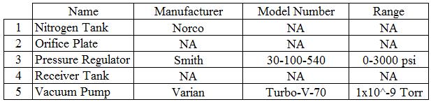
27 Chapter III: Description of Hardware This section includes information about the hardware, its manufacturer, model number, range, and the measurement uncertainties if applicable. This information can be used to replicate this experiment or obtain further information on the hardware. A hardware identification photograph and table, as shown in Figure 3, shows where the hardware is located and lists the hardware s manufacturer, model number, and range. A piping and instrumentation diagram, as shown in Table 2, shows how the hardware and instruments connect together. A table summarizing all of the lines lengths and inside diameters can be found in Appendix E. 15

28 Figure 3, Hardware Identification 16

29 Table 2, Piping, Hardware, and Instrumentation Diagram A gas bottle is to provide pressured nitrogen as the working fluid for the experiment. Air is 78 percent nitrogen, which is a close approximation for pure nitrogen, but to render more accurate results, 99.99% pure commercial grade nitrogen gas will be used as the test gas. A nitrogen bottle, provided by the company Norco, was used as the 17

30 source of nitrogen for this experiment. The pressure just upstream of the orifice was maintained at around 20 psig using a regulator. An orifice plate, as shown in Figure 4, was constructed with a hole drilled in the center of a circular plate with the desired drill bit size. Figure 4, 1/64-inch Diameter Orifice Plate L.K. Spink, Reference 14, lists specifications for the sharp, square-edged, thinplate concentric orifice which is shown in Figure 5. Specification number one was ignored for the 1/16-inch, 1/32-inch, and the 1/64-inch diameter orifice plates. This was done to simplify the fabrication process and to make it easier to duplicate the results. Table 3 shows the how the orifice plates deviate from Spink s requirement. Furthermore, the data of Ward-Smith indicates that specification number one is not essential. All of the other specifications were followed. Table 3, Spink s specification number one Plate Specification (inches) Thickness d/8 D/50 (D-d)/8 1/16-inch /32-inch /64-inch

31 Figure 5, Orifice Plate Specifications Four orifice plates were constructed: 1/16-inch hole, 1/32-inch hole, 1/64-inch hole, and a 1/64-inch hole with an exit chamfer. The 1/64-inch hole with the exit chamfer has a 45 degree chamfer to the axis of the pipe. The plates are approximately 2 inches in diameter and are made out of 1/8-inch thick cold rolled, low carbon steel. The d/d values are as follows: 1/16-inch -> , 1/32-inch -> , and 1/64-inch -> , where D is the inside diameter of the entrance line, and d is the diameter of the drill bits. The t/d values are as follows: 1/16-inch -> 2, 1/32-inch -> 4, 1/64-inch ->8, and 1/64-inch Chamfered -> 2 where t is the thickness of the of the plate at the orifice, and d is the diameter of the drill bits. The drill bits were purchased at Tacoma Screw Products, and the orifice plates were cut out on a CNC plasma table, and the holes were drilled with a drill press. 19

32 The method used to verify the orifice area and level of uncertainty on the area is known as pixel counting. This procedure is discussed in the Appendix A. The level of uncertainty of the orifice area and diameter is shown in Table 4. Table 4, Uncertainty of Orifice Area and Diameter A pressure regulator was required for the experiment to provide a constant upstream pressure. The orifice mass flow rate will only remain constant if the upstream pressure remains constant. A pressure regulator was fitted on the nitrogen bottle and was set to 20 psig. The pressure regulator used is a Smith model number with a 3000 psig max pressure inlet, a psig delivery pressure, and a +/- 2% of actual gauge reading for both the pressure regulator and flow gauges. A receiver tank was also required to collect and contain the nitrogen passed from the orifice plate. This receiver tank was constructed to withstand a negative pressure, close to a perfect vacuum, with only a negligible change in volume. The tank was fabricated for another experiment, but modified for this experiment to house all of the required fittings. It was constructed of ¼-inch thick stainless steel with a groove for an O-ring to seal the lid to the body. The volume of the receiver tank, and the remaining 20

33 volume downstream of the orifice plate was found to be ft 3, and the uncertainty was found to be +/ ft 3. The procedure for measuring the volume and determining its uncertainty can be found in Appendix A. A vacuum pump was used for this experiment. It was connected to the receiver tank with a valve in between the receiver tank and the vacuum pump. The valve was closed during testing, which limited the control volume to that downstream of the valve. A Varian Turbo-V-70 vacuum pump was used with k-type vacuum fittings. These fittings use a tightening collar and a rubber O-ring gasket. The rubber O-ring gasket should have vacuum grease applied to it, to seal and help prevent leaks. The vacuum pump must be able to remove the majority of air from the receiver tank to produce accurate results. The vacuum manufacturer reports being able to reach vacuum pressures as low as 1x10-9 Torr, however these pressures were never reached. While purging the experimental apparatus of air, the pressure would reach 3x10-3 Torr which is equivalent to 5.8x10-5 psi. It was calculated, using the ideal gas equation, that the amount of air that remained after evacuating the experimental apparatus after one purge was x10-7 lbm. A second purge was performed to reduce that amount to practically zero. 21

34 Chapter IV: Description of Instrumentation This section includes information about the instrumentation used with the instrument s manufacturer, model number, range, and its measurement uncertainty. This information can be used to replicate this experiment or obtain further information on the instrumentation. Below is an instrumentation identification photograph and table, as shown Figure 6, that shows where the instruments are located and the instrument s manufacturer, model number, range, and uncertainty. A piping and instrumentation diagram, as shown in Table 2, shows how the hardware and instruments connect together. 22

35 Figure 6, Instrumentation Identification A barometer was required for this experiment, because both differential pressure transducers reference atmospheric pressure. This allowed the pressure readings from the transducers to be standardized for calculations. The barometer that was used is a Conex Electro-Systems model JDB-1with a range of 9.8 to 15.2 psia and an uncertainty of +/ psi. The barometer displayed inches of mercury during the experiment, which is the local atmospheric pressure adjusted to seal level. The true atmospheric pressure at the elevation of Pocatello (4464 ft) is psia. This pressure reading was checked with conditions at the Pocatello airport where the sea level adjusted atmospheric pressure was recorded as inches of Mercury. At an elevation of 4,478 ft (Appendix E) the local atmospheric pressure is psia. The difference between the two measurements could be due to elevation differences or a local high or low pressure region. The reading from the barometer along with its reported uncertainties will be used in the calculations. A data acquisition system was used to collect the upstream temperature and pressure readings, along with the downstream temperature and pressure readings during 23

36 the duration of the test. In this experiment, a Graphtec midi Logger GL820 was used. The data acquisition system (DAQ) recorded measurements every 250 ms without any filters. The settings are shown in Figure 7, in the header of the recorded data. The owner s manual reported a 0.1% uncertainty of the full scale voltage. For both transducers, a 50 Volt range was used. This means that the voltage uncertainty equals ± 0.05 volts. This correlates to ± psi for the 25 psi differential pressure transducer (DPT), and ± psi for the 300 inches of water DPT. This does not take into account the uncertainty of the DPT itself. Figure 7, DAQ Output Data The owner s manual of the DAQ also reported for a k-type thermocouple for the range of -100 C < T < 1370 C, the uncertainty is ± (0.05% of reading + 1.0) C. The largest temperature reading was just above room temperature, which means that the 24

37 uncertainty for the thermocouples were ± 1.0 C or ± 1.8 F. This does not take into account the uncertainty in the thermocouple itself. Two differential pressure transducers were used to determine the upstream and downstream pressures. Both transducers referenced atmospheric pressure. The upstream pressure transducer had a range of 25 psid and the downstream pressure transducer had a range of 300 inches of water or psi. These transducers were connected to the data acquisition system electrically. The two DPTs that were used for this experiment were Omega Model-PX771A DPTs. The operation manual reported ± 0.15% of the upper range limit. The level of uncertainty for the 25 psid DPT is ± psi, and level of uncertainty for the 300 inches of water DPT is ± psi. This does not take into account the uncertainty in the DAQ for the DPTs. A pressure calibrator was used to calibrate the DPTs. A Beta Gauge PI PRO calibrator with a +/- 0.05% FS, was connected with a pressure tube fitting to each DPT. The pressure calibrator had a hand pressure pump with a digital display. The calibrator would display the pressure regardless if the hand pump was used or not. The DAQ displayed the DPTs pressure reading, which was then compared to the pressure calibrator reading. This process verified that the DPTs and the DAQ for the pressure measurements were calibrated and producing accurate readings. The calibration procedure is discussed in Appendix B. With the DPTs calibrated, the uncertainty for DPTs was assumed to be the uncertainty of the pressure calibrator. The uncertainty for the 25 psid DPT is considered 25

38 to be ± psi, and the uncertainty for the 300 inches of water DPT is considered to be ± psi. To find the total uncertainty on the pressure readings, the uncertainty of the DAQ, barometer, and the DPT must be combined into a total uncertainty. The total uncertainty for the pressure readings is calculated by taking the square root of the sum of squares, which is shown in Table 5. A power source of at least 8 volts must be supplied to the differential pressure transducers in order to power them up. The power supply used is a BK Precision model number 1710A 30B/1A with a 0-30 volt range. Two k-type thermocouples were used to determine the upstream and downstream temperatures of the nitrogen during the test duration. These thermocouples were connected to the data acquisition system. The thermocouples were produced at Idaho Laboratories, located in Idaho Falls, and were designed for a Swagelok fitting that allows the thermocouple to slide in as far as needed. The thermocouple manufacturer reported, for the range of 32 F to 100 F, an uncertainty of +/- 1 F. The experiment stays well within this temperature range. This uncertainty does not take into account the uncertainty in the DAQ for the thermocouples. The total uncertainty for the temperature readings is calculated by taking the square root of the sum of squares, which is also shown in Table 5. 26

39 Table 5, Pressure and Temperature Uncertainties 27

40 Chapter V: Setup and Test Procedure Test Setup This section includes information on how the experimental apparatus was setup. It details how each piece of equipment connects to surrounding equipment either by electrical connections or by piping or fittings. The experimental apparatus, as shown in Figure 8, was assembled in the Idaho State University s fluid and thermodynamics laboratory. Figure 8, Experimental Apparatus The function of the DAQ was to take voltage measurements from the thermocouples and DPTs and then translate that into temperature and pressure readings. The DAQ contains channel terminals. Each channel terminal consists of a positive and negative terminal. The instrumentation was connected to the DAQ terminals per the DAQ 28

41 requirements (see Figure 9 or to the Omega differential pressure transducer wiring diagram as located in the Appendix E). Figure 9, DPT wiring to DAQ The wiring diagram indicates that a 250 ohm resistor is to be placed between the positive and negative terminals on the DAQ for the DPTs, thus forming a 250 ohm resistance bridge between the two terminals. Photographs of the wiring connections are given in Figure

42 Figure 10, DAQ wiring The manual for the DAQ instructs the user on how to properly setup a thermocouple and DPT to the DAQ. The DAQ has factory settings for varying thermocouple types, and only requires a simple setting change to accommodate the k- type thermocouple. The setup of the DPT to the DAQ, is more complicated. Each DPT has a working range. For instance, the upstream DPT has a pressure range of 0 to 25 psid, and a voltage range of 1 to 5 volts. This means that if the DAQ is reading 1 volt, then the pressure is 0 psid, or if the DAQ is reading 5 volts, then the pressure is 25 psid. The DPT response is linear between these end points. This allows the DAQ to use these upper and lower limits to convert a voltage measurement into a pressure reading. 30

43 The DPTs each have two pressure ports and four electrical terminals. They have a high and low pressure port which allows only one direction of movement. The upstream DPT high pressure port was connected to the upstream line. It was decided to have the low pressure port reference atmospheric pressure, so no connection on this port was necessary. The downstream DPT low pressure port was connected to the receiving tank, because the tank experienced negative gage pressures. The high pressure port referenced atmospheric pressure, so no connection on this port was necessary. Teflon tape or pipe dope should was used on the threads of these fittings to prevent leaks. The DPT to DAQ calibration process is discussed in Appendix B. The DPT electrical terminal consists of a ground, negative, positive, and a V terminal. It both connects to the DAQ and power supply, as shown in Figure 9. To see full diagram and wiring instructions, refer to the Omega DPT wiring diagram in Appendix E. A photograph of the wiring and connections for the DPTs can be seen in Figure

44 Figure 11, DPTs wiring and connections The entrance line to the orifice plate must house a thermocouple and a pressure tap fitting. The thermocouple was placed far enough away from the orifice plate, so as to not cause flow disturbance near the orifice. A Swagelok tee fitting was used for both the thermocouple and pressure tap. The thermocouple was placed 4 feet upstream of the orifice plate, and the pressure tap fitting was placed 3.5 inches upstream of the orifice plate. The entrance line to the receiver tank can be seen in Figure

45 Figure 12, Entrance Line The orifice plates were located between the entrance line and receiver tank in a bolt flange fitting. The bolt flange fitting consisted of two heavy duty flanges with a bolt pattern and sealing gaskets. The orifice plate was placed between sealing gaskets, which was centered in between the two flanges. The bolts tightened the two flanges together, thus sealing the flange to the seals and the seals to the orifice plate. By using a bolt flange, it allows an orifice plate to be removed and installed again with little effort. This setup is shown in Figure

46 Figure 13, Orifice plate setup The DPTs call for an excitation voltage somewhere between 8 and 24 volts. It was decided to use 10 volts to excite or power up the DPTs. The power supply was connected to the DPTs and DAQ as required by the equipment specifications, as shown in Figure 9, or in the Omega differential pressure transducer wiring diagram given in Appendix E. A photograph of the power supply is shown in Figure 14. Figure 14, Power supply wiring Two thermocouples were used for this experiment, one for the upstream line, and the other for the receiver tank. Both thermocouples were designed for a Swagelok fitting that allowed the thermocouple to slide in as far as needed and then lock and seal into place. The thermocouple wire connections to the DAQ, are shown in Figure

47 Two different types of leak tests were performed on the experimental apparatus, and descriptions of both are given in Appendix B. The leak tests confirmed the experimental apparatus to be leak free. Test Procedure The test procedure used for these experiments follows: (1) Before attaching nitrogen bottle to the upstream line, the nitrogen valve was opened and the regulator pressure was set to 20 psig. Next, the nitrogen valve was closed and the pressure regulator was attached to the upstream line. (2) The desired orifice plate was placed in the flange with the orifice hole centered in the flange line, and then the flange retaining bolts were tightened. (3) A leak test was performed to ensure that no leaks were present. Refer to Appendix B for leak testing procedures. (4) The valve located between the receiver tank and vacuum pump was opened. (5) The vacuum pump was turned-on and the pump depressurized the receiver tank to the minimum level achievable with this hardware configuration. Refer to the Description of Hardware section for this vacuum pressure. (6) The valve located between the receiver tank and vacuum pump was closed. (7) To further reduce the quantity of air in the receiver tank, the nitrogen valve was opened and nitrogen was allowed to enter the receiver tank. The nitrogen valve was turned off when the receiver tank pressure reached around 0 psig. (8) The vacuum line valve was slowly opened. The valve must be opened slowly, so as to not damage the turbo blades in the vacuum pump. 35

48 (9) The vacuum pump was turned-on and the receiver tank was depressurized to the minimum pressure level a second time to minimize the quantities of gas components that are not nitrogen. The vacuum line valve was closed. (10) The data acquisition system was initiated and began to record data. (11) The nitrogen bottle valve was opened and nitrogen began to flow through the orifice plate and into the receiver tank. (12) Once the receiver tank pressure was 0 psig (the DPTs range limit), the data acquisition system recorder was switched off. (13) The test run was completed when the nitrogen bottle valve was closed. (14) If another test run was to be performed, the vacuum line valve was slowly opened. The valve must be opened slowly, so as to not damage the turbo blades in the vacuum pump. (15) Repeat steps 2-14 to test the next orifice plate. 36

49 Chapter VI: Methodology The main reasons for using a critical flow orifice to measure mass flow are simplicity, low cost, and quick turnaround: (A) Simplicity: mass flow can be measured by knowing only the fluid properties, the thermodynamic state upstream of the orifice, and the geometry of the orifice and upstream piping. The downstream pressure does not affect the measurement if the orifice is choked. (B) Low Cost: an orifice plate and the upstream piping can be constructed and assembled at almost the lowest cost of any flow measuring instrumentation. (C) Quick Turnaround: A critical orifice plate can quickly be constructed. Zucker Equation By using compressible fluid flow techniques and equations, the mass flow rate can be determined. Taking Zucker and Biblarz s equations, Reference 15 Equation 1, Mach Number M = V a Equation 2, Speed of Sound a = γrt Equation 3, Mass Flow Rate m = ρva Equation 4, Ideal Gas 37

50 ρ = P RT and combining, simplifying, and solving for the mass flow rate results in Equation 5, Ideal Mass Flow Rate m = PAM γ RT where m is the mass flow rate, P is the pressure, A is the area of the orifice, M is the mach number at the orifice (M=1 for choked flow), γ is the specific heat ratio, R is the gas constant, and T is the temperature. Equation 5 assumes that nitrogen is a perfect gas and that the conditions (temperature and pressure) are at the location where the Mach number is 1. In order to use this equation, the temperature and pressure at the throat of the orifice are required. And therefore Equation 5 is impractical to use in most application and will not be used in this application. A similar equation that assumes the Mach number is 1, but that the temperature and pressure is known as a stagnation upstream condition is Equation 6, Zucker's Critical Mass Flow Rate 1 1 m = AP t [ γ T t R ( 2 γ+1 2 γ + 1 ) γ 1 ] where P t is the upstream stagnation pressure, and T t is the upstream stagnation temperature. This equation can be found in Zucker and Biblarz, 2002, equation 5.44b. It has been found that in order to render accurate results with this equation, a discharge coefficient must be used. Rearranging, manipulating, and adding a discharge coefficient to Equation 6 results in 1 This equation is taken from Zucker and Biblarz, 2002 and will be identified in this thesis as the Zucker equation. 38

51 Equation 7, Zucker's Critical Mass Flow Rate with Discharge Coefficient 1 m = C d A [γρp t ( 2 γ+1 2 γ + 1 ) γ 1 ] where C d is the discharge coefficient, and ρ is the upstream stagnation density. Reference 6 states that for a sharp edge orifice C d = if 1 < t d < 10 where t is the thickness of the orifice plate, and d is the diameter of the orifice. If this discharge coefficient, the area equation of the orifice, and the specific heat ratio of nitrogen is substituted into Equation 7 and then simplified, results in Equation 8, Zucker's Critical Mass Flow Rate Simplified m = ( )d 2 ρp t where d is the diameter of the orifice. This equation is only valid for nitrogen and an orifice plate that meets the above mentioned criteria. Zucker s equations use stagnation conditions verses static conditions. A correctional factor, given by R.W. Miller, 1983 (Reference 16), may be applied to transform the measured static pressure to total pressure P t = [1 + γ 2 ( 2 γ+1 4 γ + 1 ) γ 1 d ( D ) ] P s where P s is the static pressure, and P t is the total pressure. The correctional factor was applied to Spink s equation and found to have negligible effect on the calculated results. 39

52 Spink Equation Another method to determine the mass flow rate through the orifice is to use L.K. Spink s equation (Reference 14, equation 56) Equation 9, Spink's Critical Mass Flow Rate W h = 359 Y T S P D 2 F a γ f1 p f1 where W h is the hourly rate of flow in pounds, Y T is the expansion factor at the critical pressure ratio for throttling orifices, S P is the K 0 β 2 for full-flow taps, K 0 is the coefficient of discharge including the velocity of approach, i.e., the flow coefficient, β is the ratio of the orifice throat diameter to the diameter of the upstream pipe, D is the actual inside diameter of the pipe, F a is the factor for temperature expansion of the orifice, γ f1 is the specific weight for the flowing fluid at upstream conditions in pounds per cubic foot, and p f1 is the upstream static pressure in psia. Y T S P can be found using Figure B-2525 (Reference 14 or Appendix E) as an approximation of air, or using this equation (Reference 14, equation 53) Equation 10, Spink's YtSp Y T S P = 4.81D 2 F a F tf F pv p f1 m w where Y T S P is the combined factor, F tf is the flowing temperature factor, F pv is the supercompressiblity factor, and m w is the molecular weight. When using Figure B-2525, Y T S P is found by using a d/d ratio where d is the orifice diameter and D is the entrance line diameter. Figure B-2525 shows a minimum d/d value of This means that the graph must be extrapolated to find Y T S P for the 1/32-inch and 1/64-inch orifice plates. Values of Y T S P and d/d were placed in excel from 40 W h

53 Figure B-2525 to produce a power function trend line equation (extrapolation equation) and graph, as shown in Figure 15. Figure 15, YtSp Trendline Graph Using the displayed equation in Figure 15, Y T S P was calculated and is shown in Table 6. This same equation was substituted into Equation 9. This would allow the results to be calculated without having to look up a new Y T S P value for a differing orifice size. Table 6, Extrapolated YtSp value for the 1/32-inch & 1/64-inch Discussion of Differences Between Zucker and Spink Equations The Zucker and Spink equations are surprisingly different and thus should be examined to identify the correspondence between terms. To accomplish this task, because both equations calculate the critical flow through an orifice plate, the two 41

54 equations are set equal to one another while adding a δ to the right-hand-side to represent the quantitative difference between the two equations. If the two equations are identically equal then the residue, when evaluated, will be identically equal. If the two equations are not identically equal then the two sides can be compared to establish the ratio be one to the other. The unlike terms are then examined one-by-one. To simplify the comparison the form of the Zucker equation given in Miller is used to compare to the Spink equation where the two equations are cast in a form where the same units are used for the primary variables, i.e., the units of static pressure (P s ) are lbf/in 2, the units of density (ρ) are lbm/ft 3, the units of mass flow rate (m ) are lbm/s, and the units of diameter (d or D) are in 2. In the following expression the Zucker equation is placed on the left and the Spink equation on the right: Cd 2 Z f Y CR ρ F TP P s = Y T S P D 2 F a ρ P s + δ where for the example given here, the gas is nitrogen, the orifice diameter is 1/16- inch, the upstream pipe inner diameter is inch, and the ratio of specific heats for nitrogen is 1.4: d = diameter of orifice (inches) = 1/16 inch = inch D = diameter of the piping upstream of the orifice (inches) = inch β = d/d = ratio of the orifice diameter to the upstream piping diameter = C = discharge coefficient for orifice = Z f = compressibility factor k = ratio of specific heats = 1.4 for nitrogen 42

55 k+1 1/2 Y CR = [ k ( 2 ) k 1 ] = [ /2 ] Z f k+1 Z f ρ = density of nitrogen (lbm/ft 3 ) F TP = [1 + k 2 ( 2 k+1 ) k+1 k 1 β 4 ] P s = static pressure upstream of orifice (lbf/in 2 ) Y T = expansion factor for throttling orifices at 50% pressure drop S P = K o β 2 for full-flow taps Y T S P = 1.942β 2 based on Figure B-2525 of Spink F a = factor for temperature expansion of the orifice plate = 80 F δ = difference between the two equations (lbm/s) The constant given on the left hand side of the Zucker equation = is a composite of the conversion factors necessary to assure unit consistency as well as to include necessary constants such as π/4 and equals π 4 [ ]1/2 = The constant given on the left hand side of the Spink equation = serves a similar purpose. Canceling like terms on the right and left sides of the above equation and inserting constants and defining expressions given above, the above equation becomes: or ( )(0.0625) 2 (0.4689) 1/2 [ (0.1453) 4 ] 1/2 = [1.942(0.1453) 2 ](0.4301) 2 + δ = δ or δ =

56 The above shows that the Zucker equation will always predict a larger mass flow rate than the Spink equation. The differences between the two equations stem from the simplifications included in the Spink equation as well as the use of an empirical approach for estimating what is in effect the discharge coefficient based on the geometry of the orifice meter coupled with ratio of the approach pipe inner diameter to the orifice diameter. In addition, two observations are important: (i) The estimate of the product of the expansion factor for throttling orifices at 50% pressure drop and factor for using fullflow taps, shown in Figure 15, required a trend-line approximation for the 1/32-inch and 1/64-inch diameter orifices and (ii) the approach outlined in Spink predates the work done by Ward-Smith described earlier and recorded in Miller. These differences combine to render the Spink approach to be less accurate than the Zucker equation. Experimentally-Measured Mass Flow Equations 5, 7, and 9 indicate that the testing apparatus must measure upstream pressure and temperature. Therefore a thermocouple and differential pressure transducer port were placed in the upstream line to continually monitor the temperatures and pressures with time, as noted in Chapter IV. The equations used to calculate the predicted mass flow rate require the diameter of the orifice. The diameter of the orifice can be approximated by using the diameter size of the drill bit that drilled the orifice. However, the actual orifice size will most likely be larger than the drill bit size due to drill bit over sizing and drill bit wobble. The area of the orifice is calculated by Equation 11, Area of a Circle A = π 4 D2 44

57 where A is the area of the orifice, and D is the diameter of the orifice. The equation can be rearranged to Equation 12, Area of a Circle Rearranged D = 4A π which if the actual area can be determine by some method, then a correctional diameter can be solved for and then inserted into the mass flow rate equations to render a more accurate calculation. One method used to more accurately determine the area of an object is by counting digital pixels. This method is described in Appendix A. The next mathematical step in this process is to find an equation that will solve for the actual mass flow rate. This flow rate is determined by the nitrogen that leaves the orifice plate and gathers in the receiver tank. There must be a way to determine how much mass is actually in the receiver tank, or how the mass in the receiver tank is changing with time. Combining these two equations Equation 13, Mass m = ρ Equation 4, Ideal Gas ρ = P RT and solving for m results in Equation 14, Mass using Ideal Gas m = P RT 45

58 where m is the mass, P is the pressure, is the volume of the receiver tank, R is the gas constant, and T is the temperature of the gas. To find the mass flow rate use or Equation 15, Mass Rate m = m t Equation 16, Mass Flow Rate for Constant Volume m = R (P 2 T 2 P 1 T 1 ) t 2 t 1 where t is the time, and subscript 1 is the condition at state 1, and subscript 2 is the condition at state 2. The volume and gas constant variables remain constant between state 1 and state 2. This is why the volume and gas constant variables are factored outside of the equation. This equation was formed by using the ideal gas equation, thus it assumes that nitrogen is an ideal gas. To render a more accurate result, an equation of state tailored for nitrogen could be used. The Benedict-Webb-Rubin equation 3-26 (Reference 17), is an equation better tailored for nitrogen, P = R ut v Equation 17, Benedict-Webb-Rubin + (B 0 R u T A 0 C 0 1 T 2) v 2 + br ut a + aα v 3 v 6 + c v 3 T 2 (1 + γ v 2 ) e γ/v 2 where P is the pressure, R u is the universal gas constant, T is the temperature, v is the specific volume per unit mole, and the rest of the variables are constants for nitrogen that can be found in Table 3-4(b) of Reference 17. Example problem 3-13 compares the Benedict-Webb-Rubin equation to experimental data of nitrogen at 10,000 kpa and at

59 K. It places this equation with a 0.09 percent error, which it states, is rather impressive The Benedict-Webb-Rubin equation does an excellent job of predicting gas behavior when the gas is at extreme or critical conditions. The ideal gas equation is unable to produce accurate results when this is the case. The ideal gas equation solutions were compared with the Benedict-Webb-Rubin equation solutions for this experiment. It was found that both equations produced the same results with minimal deviation. This is because the nitrogen remains near room temperature conditions. For simplicity, the ideal gas equation will be used to calculate the upstream and downstream conditions in place of the Benedict-Webb-Rubin equation. An investigation of uncertainty produced by using the ideal gas equation also was taken into account. A compressibility factor is often assigned to the ideal gas equation for a specific gas and operating condition. The compressibility factor converges to one as the pressure approaches zero gage pressure. Thus the ideal gas equation has a minimal, and for the purposes of this research, negligible uncertainty. Therefore the ideal gas equation will be used to calculate the upstream and downstream conditions in place of the Benedict-Webb-Rubin equation or by using a compressibility factor. Equations 14 and 16 indicate that in order to calculate the mass in the tank, the testing apparatus must measure the receiver tank temperature and pressure. A thermocouple and differential pressure transducer port was placed in the receiver tank to continually monitor the tanks temperature and pressure with time. The equations also indicate that the volume downstream of the orifice plate must be known in order to calculate the mass flow rate. The volume downstream of the orifice 47

60 plate consists of the receiver tank, the vacuum line, the pressure line to the DPT, and the volume in the DPT. To calculate the downstream volume using geometry and measurements would be time consuming and not very accurate. A more accurate method to determine the volume downstream of the orifice plate is to use a liquid such as water. Water can be added to the receiver tank, vacuum line, pressure line, and the DPT, and then the volume of the water can be measured using graduated cylinders. This process can be found in Appendix A. Measurement and Calculational Uncertainties Equations 5, 7, and 9 all assume that no errors or uncertainties reside in the variables. All measurements and instruments produce errors, so an uncertainty interval must be developed to model these errors. The ASME national standard for computing the measurement uncertainty of fluid flow in a closed conduit (Reference 18) describes the procedure to correctly capture uncertainties in flow calculations and is used to compute the measurement uncertainty for both the experiment and the calculations in this thesis. The ASME national standard states: Uncertainty is a function of the measurement process. It provides an estimate of the error band within which the true value for that measurement process must fall with high probability. Errors larger than the uncertainty should rarely occur. On repeated runs within a given measurement process, the parameter values should be within the uncertainty interval. Run-to-run differences between corresponding values of the parameter should be less than the uncertainty for the parameter. The standard then describes how the errors in the measurements are propagated through the function, and how this effect can be approximated by using a Taylor series expansion 48

61 method. The standard gives an example problem demonstrating this technique for a choked venturi. Using Reference 18, the Taylor series expansion equation was tailored for Equation 7, Equation 18, Taylor Series Expansion Tailored for Eq. 7 S m = ( 2 m S d ) + ( 2 m S d P ) + ( 2 m S P T ) T where S m is the mass flow rate precision index, d is the orifice diameter and S d is its precision index, P is the upstream pressure and S P is its precision index, and T is the upstream temperature and S T is its precision index. Notice that the density is not included in equation 18 since it is a direct function of the fluid pressure and temperature via the ideal gas law. Also, as noted in the ASME national standard, the uncertainties of both the ratio of specific heats and the compressibility are both negligible when evaluated at the proper thermodynamic conditions (see Reference 18, Section , page 41). The precision index equation was similarly tailored for Equation 9 Equation 19, Taylor Series Expansion Tailored for Eq. 9 S m = ( 2 m S d ) + ( 2 m S d P ) + ( 2 m S P T ) T where S m is the mass flow rate precision index, d is the orifice diameter and S d is its precision index, P is the upstream pressure and S P is its precision index, and T is the upstream temperature and S T is its precision index. The precision index equation tailored for Equation 16 is 49

62 Equation 20, Taylor Series Expansion Tailored for Eq. 16 S m = ( 2 m S V ) + ( 2 m S V P ) + ( 2 m S P T ) T where S m is the mass precision index, V is the receiver tank volume and S V is its precision index, P is the upstream pressure and S P is its precision index, and T is the upstream temperature and S T is its precision index. 7 becomes After computing the partial derivatives and applying the constant values, Equation S m = ( d2 P 2 2 S d ) + ( d4 2 S P R T R T ) + ( d4 P 2 2 S T R T 3 ) Equation 9 becomes ( d P S d 2 ( P T )) S m = [ S P 2 ( and Equation 16 becomes ( d ( P 0.5 T ) P 0.5 ) + ( d P 0.5 ( P3 d S T 2 T 4 ( P T ) ) ( P 0.5 T ) T ) ) 2 + ] 50

63 S 2 V ( P 2 T P 2 1 S m = [( 2 T ) 1 R 2 (t 2 t 1 ) 2 ) + ( V 2 2 S P R 2 T 2 1 (t 2 t 1 ) 2) + ( V 2 2 S P R 2 T 2 2 (t 2 t 1 ) 2) P 2 1 S 2 T V 2 + ( R 2 T 4 1 (t 2 t 1 ) 2) + ( P 2 2 S 2 T V 2 R 2 T 4 2 (t 2 t 1 ) 2)] 1 2 The uncertainties associated with the temperature, pressure, orifice diameter, and receiver tank measurements are listed in the Hardware and Instrumentation sections and are also summarized below on Table 7. Table 7, Precision Index/Uncertainty Summary 51

64 Chapter VII: Results The experiment, as explained in the Test Procedure section, consisted of four separate tests with four different orifice plates. The orifice sizes that were used were a 1/16-inch orifice, a 1/32-inch orifice, a 1/64-inch (#78) orifice, and a 1/64-inch (#78) orifice with an exit chamfer. Each test was run with an upstream pressure between 18 psig and 20 psig. During the duration of the test, the downstream pressure was initially around 1 psia and then increased to 13 psia at the end of the test. The mass flow rate was calculated using Zucker (Equation 7), Spink (Equation 9), and the ideal tank equation (Equation 16). The results are shown on the graphs below, see Figures 15, 16, 17, and 18. Each orifice plate graph compares the mass flow verses time for each of the three equations. A second graph plots the upstream pressure during the duration of the test. 52

65 Figure 16, 1/16-inch Orifice Plate Test Graphs 53

66 Figure 17, 1/32-inch Orifice Plate Test Graphs 54

67 Figure 18, 1/64-inch Regular Orifice Plate Test Graphs 55

68 Figure 19, 1/64-inch Chamfered Orifice Plate Test Graphs It is important to verify that critical flow is occurring during the test. The graphs show that the mass flow rate for each orifice remains constant with a slight decline. When looking at the upstream pressure verses time graph, the upstream pressure decreases with time. This explains why the mass flow rate was decreasing for each test. If the upstream pressure decreases then the mass flow rate will also decrease. If a high quality pressure regulator would have been used, then the upstream pressure would have remained constant, and in turn, caused the mass flow rate to also remain constant. It is interesting to note that the tank equation curve is very noisy. The literature review mentioned this, A related disadvantage of the critical flow meter is the acoustical disturbance created in the downstream fluid The resulting shock waves cause acoustical noise and turbulence, which may affect apparatus performance and downstream measurements in some applications (Reference 4). For example, the tank temperature 56

69 data verses time was plotted for the 1/16-inch orifice plate and is shown in Figure 20. This graph shows the level of noise present in the temperature measurements. Figure 20, Tank Temperature Graph It was observed that the 1/16-inch diameter orifice discharged the nitrogen 4 times faster than then the 1/32-inch diameter orifice, and 16 times faster than the 1/64-inch diameter orifices. The flow rates differ by a ratio of the square of the respective diameters. This is why a diameter twice as big produces a mass flow rate four times greater than the diameter twice as small. Equations 7 and 9 were used to calculate the theoretical mass flow rate, while Equation 16 was used to calculate the actual mass flow rate. Equation 5 was not used, because it was not possible to measure the flow conditions at the throat of the vena contracta with available instrumentation. This is due to the assumption than no losses are present in the form of a discharge coefficient. When calculating the actual conditions from Equation 16, the time step must receive special attention. If the time step is too small, then Equation 16 will produce poor results. This is due to instrumentation noise. 57

70 The DAQ recorded conditions every ¼ of a second, so if that were to be used as the calculating time step, then the difference would negligible. For this reason, the 1/16 orifice plate was calculated using a 5 second time step, the 1/32 orifice plate was calculated using a 10 second time step, and the #78 orifice plate was calculated using a 15 second time step. The calculated average mass flow rates with uncertainties are reported in Table 8. Table 8, Average Mass Flow Rates with Uncertainties 58

71 Chapter VIII: Conclusions Conclusions fall into two distinct areas regarding: (i) the uncertainties in the critical mass flow rate that should be expected by a researcher using critical flow orifices when using standard calculation practices while observing recommended experimental standard practices and (ii) observations regarding the advantages of using critical flow orifices vis-à-vis other critical flow measurement devices such as a critical flow nozzle or venture. Uncertainties in the Critical Mass Flow Rate Calculated Using Standard Practices The calculational uncertainty using Zucker s equation was found to be ±1.5% for the 1/16-inch diameter orifice,, ±2.1% for the 1/32-inch diameter orifice, and ±2.9% for both of the 1/64-inch diameter orifices. The calculational uncertainty using Spink s equation was found to be ±5.1% for the 1/16-inch diameter orifice,, ±10.6% for the 1/32- inch diameter orifice, and ±17.0% for both of the 1/64-inch diameter orifices. As previously discussed, the Spink equation is an outdated methodology which is of limited use for the purpose of this research in part because a trend-line approximation was required to perform the mass flow rate calculations for the 1/32-inch and 1/64-inch diameter orifices. Therefore the Zucker equation is recommended and the above calculational accuracies, ranging from ±1.5% for the 1/16-inch diameter orifice to ±2.9% for the 1/64-inch diameter orifice are reasonable and acceptable for many applications. Virtues of Using Critical Flow Orifices Compared to other types of flow meters, a critical flow orifice meter is relatively simple to construct and can be constructed very quickly. In addition it is very 59

72 inexpensive to construct a critical flow orifice. For these reasons, the critical flow orifice meter may be preferred over other meters, even if it may not be as accurate. To minimize the measurement uncertainty the critical flow orifice may be calibrated in situ. Future Research Possibilities/Questions for Future Inquiry A possible future study would be to test how the mass flow rate changes as you approach the critical pressure ratio. Also, another similar future study would be to vary the upstream pressure and see if the total percent error would change. This information would be important if a critical flow orifice meter were to be used at differing upstream pressures. 60

73 References 1. Busch, Vacuum Pumps and Systems. Flow Through An Orifice: How Orifice Size is Useful in Vacuum Pump Selection. Retrieved from ough_an_orifice.pdf 2. Kurita, C.H. (1988). Critical Flow Restricting Orifices. Retrieved from 3. Urone, P & Ross, R. (1979). Pressure Change Effects on Hypodermic Needle. Critical Orifice Air Flow Rates. American Chemical Society, Volume 13, Number 3. Retrieved from 4. Perry, Jr., J. A. Critical Flow Through Sharp-Edged Orifices, Trans. ASME, 71: 737: Ward, A. & Smith, J. (1979). Critical Flowmetering: The Characteristics of Cylindrical Nozzles with Sharp Upstream Edges. International Journal of Heat and Fluid Flow, Vol:1, pp Brain, T. J. S., and Reid, J. Performance of small diameter cylindrical critical flow nozzles, National Engineering Laboratory Report 546, Deckker, B. E. L., and Chang, Y.F. An investigation of steady compressible flow of air through square edged orifices, Proc. Instn. Mech. Engrs., , 180, (Pt. 3J), Jackson, R. A. The compressible discharge of air through small thick plate orifices, Appl. Scient. Res., Section A, 1963, 13,

74 9. Grace, H.P., and Lapple, C. E. Discharge coefficients of small diameter orifices and flow nozzles, Trans. Am. Soc. Mech. Engrs., 1951, 73, Kastner, L. J., Williams, T.J., and Sowden, R. A. Critical-flow nozzle meter and its application to the measurement of mass flow rate in steady and pulsating streams of gas, J. Mech, Engng. Sci., 1964, 6, (1), Rohde, J. E., Richards, H. T., and Metger, G. W. Discharge coefficients for thick plate orifices with approach flow perpendicular and inclined to the orifice axis, National Aeronautics and Space Administration NANA TN D-5467, Zimmerman, N & Reist, P. (1984). The Critical Orifice Revisited: A Novel Low Pressure Drop Critical Orifice. American Industrial Hygiene Association Journal, Vol: 45, pp Stanton, T. E. On the Flow of Gases at High Speed. Proc. R. Soc. London 111, , Spink, L.K. (1967). Principles and Practice of Flow Meter Engineering: Ninth Edition. Foxboro, Massachusetts, USA: The Foxboro Company. 15. Zucker, R & Biblarz, O. (2002). Fundamentals of Gas Dynamics: Second Edition. Hoboken, New Jersey: John Wiley & Sons, Inc. 16. Miller, R.W., Flow Measurement Engineering Handbook, McGraw-Hill Co, page 13-4, equation 13.9, Cengel, Y & Boles, M. (2008). Thermodynamics, An Engineering Approach: Sixth Edition. New York, NY: The McGraw-Hill Companies Inc. 62

75 18. Measurement Uncertainty for Fluid Flow in Closed Conduits. ANSI/ASME MFC-2M An American National Standard. New York, NY: The American Society of Mechanical Engineers 63

76 Appendices Appendix A: Orifice Area & Downstream Volume Calculation Procedure 64

77 Pixel Counting This is accomplished by scanning an orifice plate at a high resolution. The image can then be magnified until each individual pixel can be detected and counted. A pixel that lies on the orifice region will be a different color from a pixel that lies on the orifice plate material. If a pixel lies on the edge of the orifice and the plate, the color will be in between the color of the orifice and the color of the plate. The shade of the pixel will determine how much of the total pixel area lies over the edge. Using two separate scanners, two images of a single orifice plate were used to determine how many pixels each orifice contained. The pixels that were located on the edge of the orifice were also counted. Each scanned image has a resolution in terms of dots per inch (dpi). If the resolution is 600 dpi, this means that there are 600 dots per linear inch. Two dots in the horizontal direction and two dots in the vertical direction make up a pixel. A pixel is basically a square made up of equal sides that are the length of a dot. To calculate the area of the orifice based on the number of pixels, use this equation A = # of Pixels (dpi) 2 where that area is reported in squared inches. Figure 21 is a zoomed printed image produced from both scanners. It shows the contrast between the hole and orifice plate. 65

78 Figure 21, Pixel Counting The circumference of the orifice is directly related to the number of pixels that occupy the edge of the orifice. By using the circumference of the orifice, the number of dots per inch can be calculated along with the number of pixels that occupy the edge. The calculated number of pixels on the edge is very close to the number of pixels physically counted on the edge of the orifice on the scanned image. It will be assumed that the area of the orifice is calculated based on the diameter of the drill bit that drilled the hole plus or minus the area of the pixels that occupy the edge of the orifice. It was determined that level of uncertainty of the orifice area is as follows: 1/16-inch orifice > / in 2, 1/32-inch orifice > / in 2, 1/64-inch orifice > / in 2. 66

79 Determining the Volume and Uncertainty Downstream of the Orifice Plate The volume downstream of the orifice was determined by adding water to the receiver tank, vacuum line, DPT line, and the DPT, and then measuring this water with a 2000 ml graduated cylinder. Water was added to the receiver tank through the vacuum line, and the air was bled from the lid surface by loosening the fittings on the lid. The tank was constantly moved and vibrated to work the air bubbles out of the lid surface. The 2000 ml graduated cylinder that was used, had 20 ml incremental measuring lines. All measurements were made by using the 20 ml lines on the graduated cylinder. Using a +/- 20 ml for each individual measurement with 14 total measurements, equals +/- 280 ml or +/ ft 3 level of uncertainty on the total volume. The total volume was found to be Liters or ft 3. Another method for determining the volume of the receiver tank was used. The receiver tank was weighed initially dry, and then again after water was added. This method proved to have too high of an uncertainty, because a low precision scale that was used. An uncertainty of 1 lb of water converts to 2 cups of volume. If a more precise scale had been used, this method would have worked. 67

80 Appendix B: Calibration Process & Leak Test 68

81 Calibration Process The thermocouples, DPTs, and the DAQ all must calibrated together in order to produce accurate results. The DPTs were calibrated by using a pressure calibrator, as seen in Figure 22. A pressure calibrator is a trusted device that shows the actual pressure reading in comparison to the DPT s reading. This pressure calibrator was connected to each DPT for calibration. The DAQ that was used for this experiment had an upper and lower range setting to automatically convert a voltage measurement to a pressure reading. Both DPTs pressure readings showed deviation from the calibrator readings near the beginning and ending of the of the DPT s range. It was determined to ignore data received from the DAQ at these upper and lower ranges. It was confirmed that the DPTs, within the acceptable ranges, were calibrated and producing pressure readings accurately. Figure 22, Pressure Calibrator The thermocouples were calibrated by using a trusted/calibrated thermometer. An ice bath and hot water bath were also used with the calibrated thermometer and thermocouple, to verify that the thermocouples were producing accurate temperature 69

82 readings. This calibration process confirmed that the thermocouples were calibrated and working properly. Leak Test Two types of leak tests were performed to verify that the test apparatus was not leaking from the fittings or connections. The first leak test was accomplished by adding pressurized air (40 psig) to the receiver tank and using a water/soap solution to detect leaks in the form of bubbles. Initially, Teflon tape was used on the threaded connections, but the bubble leak test revealed that the Teflon tape did not prevent leaks. The Teflon tape was then replaced with a pipe thread dope sealant. The leak test was performed again, and found that the pipe dope sealed and prevent leaks from occurring. This test can be seen in Figure 23. Figure 23, Bubble Leak Test The next leak test consisted of pulling a vacuum and monitoring the system pressure with respect to time. This leak test was performed in conjunction with the actual testing. The pressure in the system was reduced to 3x10^-3 Torr, and was able to 70

83 maintain that pressure for15 minutes. This leak test was repeated for each orifice plate to insure that no leaking was occurring between the flange fitting and orifice plate after changing each of the orifice plates. 71

84 Appendix C: Calculation Examples 72

85 Tank Mass Flow Equation 73

86 Tank Mass Flow Uncertainty Equation 74

87 75

88 Zucker Mass Flow Equation 76

89 Zucker Mass Flow Uncertainty Equation 77

90 Spink Mass Flow Equation 78

91 Spink Mass Flow Uncertainty Equation

92 Appendix D: Test Data Report 80

93 1/16-inch Orifice Plate Vendor GRAPHTEC Corp. Model GL820 Version Ver1.03 Sampling interval 250ms Total data points 151 Start time 11/17/ :47:56 End time 11/17/ :48:34 Trigger time 11/17/ :47:56 AMP settings CH Signal name Input Range Filter Span CH1 P TANK DC 50V Off [psi] CH2 P UPSTREAM DC 50V Off [psi] CH3 T TANK TEMP TC_K Off [degf] CH4 T UPSTREAM TEMP TC_K Off [degf] Logic/Pulse Off Data Number Date&Time ms CH1 CH2 CH3 CH4 NO. Time ms psi psi degf degf 20 11/17/ : /17/ : /17/ : /17/ : /17/ : /17/ : /17/ : /17/ : /17/ : /17/ : /17/ : /17/ : /17/ : /17/ : /17/ : /17/ : /17/ : /17/ : /17/ : /17/ : /17/ : /17/ : /17/ :

94 43 11/17/ : /17/ : /17/ : /17/ : /17/ : /17/ : /17/ : /17/ : /17/ : /17/ : /17/ : /17/ : /17/ : /17/ : /17/ : /17/ : /17/ : /17/ : /17/ : /17/ : /17/ : /17/ : /17/ : /17/ : /17/ : /17/ : /17/ : /17/ : /17/ : /17/ : /17/ : /17/ : /17/ : /17/ : /17/ : /17/ : /17/ : /17/ : /17/ : /17/ : /17/ : /17/ : /17/ :

95 86 11/17/ : /17/ : /17/ : /17/ : /17/ : /17/ : /17/ : /17/ : /17/ : /17/ : /17/ : /17/ : /17/ : /17/ : /17/ : /17/ : /17/ : /17/ : /17/ : /17/ : /17/ : /17/ : /17/ : /17/ : /17/ : /17/ : /17/ : /17/ : /17/ : /17/ : /17/ : /17/ : /17/ : /17/ : /17/ : /17/ : /17/ : /17/ : /17/ : /17/ : /17/ : /17/ : /17/ :

96 129 11/17/ : /17/ : /17/ : /17/ : /17/ : /17/ : /17/ : /17/ : /17/ : /17/ : /17/ : /17/ : /17/ : /17/ : /17/ : /17/ : /17/ : /17/ : /17/ : /17/ : /17/ : /17/ : /17/ :

97 1/32-inch Orifice Plate GRAPHTEC Vendor Corp. Model GL820 Version Ver1.03 Sampling interval 250ms Total data points 490 Start time 11/17/ :27:4 8 End time 11/17/ :29:5 1 Trigger time 11/17/ :27:4 8 AMP settings CH Signal name Input Range Filter Span CH1 P TANK DC 50V Off [psi] CH2 P UPSTREAM DC 50V Off [psi] CH3 T TANK TEMP TC_K Off [degf ] CH4 T UPSTREAM TEMP TC_K Off [degf ] Logic/Pulse Off Data Number Date&Time ms CH1 CH2 CH3 CH4 NO. Time ms psi psi degf degf 20 11/17/14 12: /17/14 12: /17/14 12: /17/14 12: /17/14 12: /17/14 12: /17/14 12: /17/14 12: /17/14 12: /17/14 12: /17/14 12: /17/14 12: /17/14 12: /17/14 12: /17/14 12: /17/14 12: /17/14 12:

98 54 11/17/14 12: /17/14 12: /17/14 12: /17/14 12: /17/14 12: /17/14 12: /17/14 12: /17/14 12: /17/14 12: /17/14 12: /17/14 12: /17/14 12: /17/14 12: /17/14 12: /17/14 12: /17/14 12: /17/14 12: /17/14 12: /17/14 12: /17/14 12: /17/14 12: /17/14 12: /17/14 12: /17/14 12: /17/14 12: /17/14 12: /17/14 12: /17/14 12: /17/14 12: /17/14 12: /17/14 12: /17/14 12: /17/14 12: /17/14 12: /17/14 12: /17/14 12: /17/14 12: /17/14 12: /17/14 12: /17/14 12: /17/14 12: /17/14 12: /17/14 12:

99 140 11/17/14 12: /17/14 12: /17/14 12: /17/14 12: /17/14 12: /17/14 12: /17/14 12: /17/14 12: /17/14 12: /17/14 12: /17/14 12: /17/14 12: /17/14 12: /17/14 12: /17/14 12: /17/14 12: /17/14 12: /17/14 12: /17/14 12: /17/14 12: /17/14 12: /17/14 12: /17/14 12: /17/14 12: /17/14 12: /17/14 12: /17/14 12: /17/14 12: /17/14 12: /17/14 12: /17/14 12: /17/14 12: /17/14 12: /17/14 12: /17/14 12: /17/14 12: /17/14 12: /17/14 12: /17/14 12: /17/14 12: /17/14 12: /17/14 12: /17/14 12:

100 226 11/17/14 12: /17/14 12: /17/14 12: /17/14 12: /17/14 12: /17/14 12: /17/14 12: /17/14 12: /17/14 12: /17/14 12: /17/14 12: /17/14 12: /17/14 12: /17/14 12: /17/14 12: /17/14 12: /17/14 12: /17/14 12: /17/14 12: /17/14 12: /17/14 12: /17/14 12: /17/14 12: /17/14 12: /17/14 12: /17/14 12: /17/14 12: /17/14 12: /17/14 12: /17/14 12: /17/14 12: /17/14 12: /17/14 12: /17/14 12: /17/14 12: /17/14 12: /17/14 12: /17/14 12: /17/14 12: /17/14 12: /17/14 12: /17/14 12: /17/14 12:

101 312 11/17/14 12: /17/14 12: /17/14 12: /17/14 12: /17/14 12: /17/14 12: /17/14 12: /17/14 12: /17/14 12: /17/14 12: /17/14 12: /17/14 12: /17/14 12: /17/14 12: /17/14 12: /17/14 12: /17/14 12: /17/14 12: /17/14 12: /17/14 12: /17/14 12: /17/14 12: /17/14 12: /17/14 12: /17/14 12: /17/14 12: /17/14 12: /17/14 12: /17/14 12: /17/14 12: /17/14 12: /17/14 12: /17/14 12: /17/14 12: /17/14 12: /17/14 12: /17/14 12: /17/14 12: /17/14 12: /17/14 12: /17/14 12: /17/14 12: /17/14 12:

102 398 11/17/14 12: /17/14 12: /17/14 12: /17/14 12: /17/14 12: /17/14 12: /17/14 12: /17/14 12: /17/14 12: /17/14 12: /17/14 12: /17/14 12: /17/14 12: /17/14 12: /17/14 12: /17/14 12: /17/14 12: /17/14 12: /17/14 12: /17/14 12: /17/14 12: /17/14 12: /17/14 12: /17/14 12: /17/14 12: /17/14 12: /17/14 12: /17/14 12: /17/14 12: /17/14 12: /17/14 12: /17/14 12: /17/14 12: /17/14 12: /17/14 12: /17/14 12: /17/14 12: /17/14 12: /17/14 12: /17/14 12: /17/14 12: /17/14 12: /17/14 12:

103 484 11/17/14 12: /17/14 12: /17/14 12: /17/14 12:

104 1/64-inch Regular Orifice Plate GRAPHTEC Vendor Corp. Model GL820 Version Ver1.03 Sampling interval 250ms Total data points 2154 Start time 11/17/ :50:32 End time 11/17/ :59:30 Trigger time 11/17/ :50:32 AMP settings CH Signal name Input Range Filter Span CH1 P TANK DC 50V Off [psi] CH2 P UPSTREAM DC 50V Off [psi] CH3 T TANK TEMP TC_K Off [degf] CH4 T UPSTREAM TEMP TC_K Off [degf] Logic/Pulse Off Data Number Date&Time ms CH1 CH2 CH3 CH4 NO. Time ms psi psi degf degf 50 11/17/14 11: /17/14 11: /17/14 11: /17/14 11: /17/14 11: /17/14 11: /17/14 11: /17/14 11: /17/14 11: /17/14 11: /17/14 11: /17/14 11: /17/14 11: /17/14 11: /17/14 11: /17/14 11: /17/14 11: /17/14 11: /17/14 11: /17/14 11: /17/14 11: /17/14 11:

105 270 11/17/14 11: /17/14 11: /17/14 11: /17/14 11: /17/14 11: /17/14 11: /17/14 11: /17/14 11: /17/14 11: /17/14 11: /17/14 11: /17/14 11: /17/14 11: /17/14 11: /17/14 11: /17/14 11: /17/14 11: /17/14 11: /17/14 11: /17/14 11: /17/14 11: /17/14 11: /17/14 11: /17/14 11: /17/14 11: /17/14 11: /17/14 11: /17/14 11: /17/14 11: /17/14 11: /17/14 11: /17/14 11: /17/14 11: /17/14 11: /17/14 11: /17/14 11: /17/14 11: /17/14 11: /17/14 11: /17/14 11: /17/14 11: /17/14 11: /17/14 11:

106 700 11/17/14 11: /17/14 11: /17/14 11: /17/14 11: /17/14 11: /17/14 11: /17/14 11: /17/14 11: /17/14 11: /17/14 11: /17/14 11: /17/14 11: /17/14 11: /17/14 11: /17/14 11: /17/14 11: /17/14 11: /17/14 11: /17/14 11: /17/14 11: /17/14 11: /17/14 11: /17/14 11: /17/14 11: /17/14 11: /17/14 11: /17/14 11: /17/14 11: /17/14 11: /17/14 11: /17/14 11: /17/14 11: /17/14 11: /17/14 11: /17/14 11: /17/14 11: /17/14 11: /17/14 11: /17/14 11: /17/14 11: /17/14 11: /17/14 11: /17/14 11:

107 /17/14 11: /17/14 11: /17/14 11: /17/14 11: /17/14 11: /17/14 11: /17/14 11: /17/14 11: /17/14 11: /17/14 11: /17/14 11: /17/14 11: /17/14 11: /17/14 11: /17/14 11: /17/14 11: /17/14 11: /17/14 11: /17/14 11: /17/14 11: /17/14 11: /17/14 11: /17/14 11: /17/14 11: /17/14 11: /17/14 11: /17/14 11: /17/14 11: /17/14 11: /17/14 11: /17/14 11: /17/14 11: /17/14 11: /17/14 11: /17/14 11: /17/14 11: /17/14 11: /17/14 11: /17/14 11: /17/14 11: /17/14 11: /17/14 11: /17/14 11:

108 /17/14 11: /17/14 11: /17/14 11: /17/14 11: /17/14 11: /17/14 11: /17/14 11: /17/14 11: /17/14 11: /17/14 11: /17/14 11: /17/14 11: /17/14 11: /17/14 11: /17/14 11: /17/14 11: /17/14 11: /17/14 11: /17/14 11: /17/14 11: /17/14 11: /17/14 11: /17/14 11: /17/14 11: /17/14 11: /17/14 11: /17/14 11: /17/14 11: /17/14 11: /17/14 11: /17/14 11: /17/14 11: /17/14 11: /17/14 11: /17/14 11: /17/14 11: /17/14 11: /17/14 11: /17/14 11: /17/14 11: /17/14 11: /17/14 11: /17/14 11:

109 /17/14 11: /17/14 11: /17/14 11: /17/14 11: /17/14 11: /17/14 11: /17/14 11: /17/14 11: /17/14 11: /17/14 11: /17/14 11: /17/14 11: /17/14 11: /17/14 11: /17/14 11: /17/14 11: /17/14 11:

110 1/64-inch Chamfered Orifice Plate Vendor GRAPHTEC Corp. Model GL820 Version Ver1.03 Sampling interval 250ms Total data points 1710 Start time 11/17/ :13:16 End time 11/17/ :20:24 Trigger time 11/17/ :13:17 AMP settings CH Signal name Input Range Filter Span CH1 P TANK DC 50V Off [psi] CH2 P UPSTREAM DC 50V Off [psi] CH3 T TANK TEMP TC_K Off [degf] CH4 T UPSTREAM TEMP TC_K Off [degf] Logic/Pulse Off Data Number Date&Time ms CH1 CH2 CH3 CH4 NO. Time ms psi psi degf degf 50 11/17/14 11: /17/14 11: /17/14 11: /17/14 11: /17/14 11: /17/14 11: /17/14 11: /17/14 11: /17/14 11: /17/14 11: /17/14 11: /17/14 11: /17/14 11: /17/14 11: /17/14 11: /17/14 11: /17/14 11: /17/14 11: /17/14 11: /17/14 11: /17/14 11: /17/14 11: /17/14 11:

111 280 11/17/14 11: /17/14 11: /17/14 11: /17/14 11: /17/14 11: /17/14 11: /17/14 11: /17/14 11: /17/14 11: /17/14 11: /17/14 11: /17/14 11: /17/14 11: /17/14 11: /17/14 11: /17/14 11: /17/14 11: /17/14 11: /17/14 11: /17/14 11: /17/14 11: /17/14 11: /17/14 11: /17/14 11: /17/14 11: /17/14 11: /17/14 11: /17/14 11: /17/14 11: /17/14 11: /17/14 11: /17/14 11: /17/14 11: /17/14 11: /17/14 11: /17/14 11: /17/14 11: /17/14 11: /17/14 11: /17/14 11: /17/14 11: /17/14 11: /17/14 11:

112 710 11/17/14 11: /17/14 11: /17/14 11: /17/14 11: /17/14 11: /17/14 11: /17/14 11: /17/14 11: /17/14 11: /17/14 11: /17/14 11: /17/14 11: /17/14 11: /17/14 11: /17/14 11: /17/14 11: /17/14 11: /17/14 11: /17/14 11: /17/14 11: /17/14 11: /17/14 11: /17/14 11: /17/14 11: /17/14 11: /17/14 11: /17/14 11: /17/14 11: /17/14 11: /17/14 11: /17/14 11: /17/14 11: /17/14 11: /17/14 11: /17/14 11: /17/14 11: /17/14 11: /17/14 11: /17/14 11: /17/14 11: /17/14 11: /17/14 11: /17/14 11:

113 /17/14 11: /17/14 11: /17/14 11: /17/14 11: /17/14 11: /17/14 11: /17/14 11: /17/14 11: /17/14 11: /17/14 11: /17/14 11: /17/14 11: /17/14 11: /17/14 11: /17/14 11: /17/14 11: /17/14 11: /17/14 11: /17/14 11: /17/14 11: /17/14 11: /17/14 11: /17/14 11: /17/14 11: /17/14 11: /17/14 11: /17/14 11: /17/14 11: /17/14 11: /17/14 11: /17/14 11: /17/14 11: /17/14 11: /17/14 11: /17/14 11: /17/14 11: /17/14 11: /17/14 11: /17/14 11: /17/14 11: /17/14 11: /17/14 11: /17/14 11:

114 /17/14 11: /17/14 11: /17/14 11: /17/14 11: /17/14 11: /17/14 11: /17/14 11: /17/14 11: /17/14 11: /17/14 11: /17/14 11: /17/14 11: /17/14 11: /17/14 11: /17/14 11: /17/14 11: /17/14 11: /17/14 11: /17/14 11: /17/14 11: /17/14 11: /17/14 11: /17/14 11: /17/14 11: /17/14 11: /17/14 11: /17/14 11: /17/14 11: /17/14 11: /17/14 11: /17/14 11: /17/14 11: /17/14 11: /17/14 11: /17/14 11: /17/14 11: /17/14 11: /17/14 11: /17/14 11: /17/14 11: /17/14 11: /17/14 11: /17/14 11:

115 /17/14 11: /17/14 11: /17/14 11: /17/14 11: /17/14 11: /17/14 11: /17/14 11: /17/14 11: /17/14 11: /17/14 11: /17/14 11: /17/14 11: /17/14 11: /17/14 11: /17/14 11: /17/14 11:

116 Appendix E: Diagrams, Graphs, Tables, etc. 104

117 Omega differential pressure transducer wiring diagrams 105

118 Spink s YtSp Graph for d/d 106

119 Pocatello Airport Conditions at Time of Testing 107

120 Experimental Apparatus Line Dimensions 108