Data Analysis I: Single Subject

Transcription

1 Data Analysis I: Single Subject

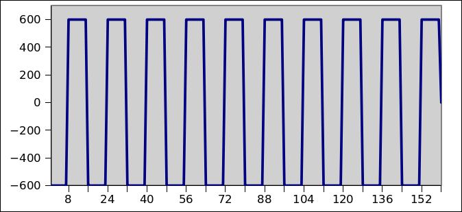
2 ON OFF

3

4 he General Linear Model (GLM) y= X fmri Signal = Design Matrix our data = what we CAN explain x β x Betas + + how much x of it we CAN + explain ε Residuals what we CANNO explain If a voxel cares about the task, then you should be able to predict its time-course from the onset and offset of the task. β captures how much of 'y' your task/design is predicting.

5 he General Linear Model (GLM) y= X fmri Signal = Design Matrix our data = what we CAN explain x β x Betas + + how much x of it we CAN + explain ε Residuals what we CANNO explain

6 he General Linear Model (GLM) yi = β0+β1x1+ εi yi Reaction time X1 Age β0, β1 are the model parameters εi is the random error; how observation deviates from population mean

7 he General Linear Model (GLM) yi = β0+β1x1+ εi Fixed: β0+β1x1 Mean of Yi (E[Yi]) Random: εi he variability of Y i (needs to have specific properties)

8 he General Linear Model (GLM) AGE Source: J Mumford

9 Statistical Analysis Conceptually the analysis is divided into 2 steps: 1. Estimation: the magnitude of the effect of interest (β) 2. Inference: assess significance of the estimated parameter

10 Ordinary Least Squares (OLS) e.g. What is the relationship tying years of MALB experience and coding efficiency?

11 Ordinary Least Squares (OLS) e.g. What is the relationship tying years of MALB experience and coding efficiency? Minimize error: Actual (i.e. Y) n 2 i n 2 e = Y i Y i i=1 n Predicted (i.e. Y-hat) i=1 2 Y i 1 X 1 i=1

12 Ordinary Least Squares (OLS) e.g. What is the relationship tying years of MALB experience and coding efficiency? Minimize error: Actual (i.e. Y) n 2 i n 2 e = Y i Y i i=1 n Predicted (i.e. Y-hat) i=1 2 Y i 1 X 1 i=1

13 Least Squares Difference Minimize error n n i=1 i=1 2 2 e = Y i Y i = Y i i X i i=1 2 i n Y i Y X X i 1= 2 Y i Y 0 =Y 1 X

14 Massive Univariate Approach y = 0 1 X 1

15 Massive Univariate Approach y = 0 1 X 1 2 X 2... p X p

16 Voxel-wise GLM y 1= 0 1 X 1,1 2 X 2,1 p X p,1 1 y 2= 0 1 X 1,2 2 X 2,2 p X p, 2 2 y 3= 0 1 X 1,3 2 X 2,3 p X p,3 3 y n= 0 1 X 1, n 2 X 2, n p X p, n n

17 Voxel-wise GLM

18 Voxel-wise GLM

19 Voxel-wise GLM

20 Voxel-wise GLM

21 Voxel-wise GLM

22 Ordinary Least Squares (OLS) Y = X Y = X X Y = X X X X X Y = 1

23 Ordinary Least Squares (OLS) Y = X = X X 1 X Y 2 1 Var = X X 1 X X X Y t= = ~ N p 2 1 Var X X

24 Ordinary Least Squares (OLS) Effect of interest Nature 1 X X X Y t= = ~ N p 2 1 X X Var Subject, scanner,... You Residuals Error (i.e., what we don't know) Design Matrix

25 Gauss Markov Assumptions Under the following assumptions, the OLS estimator is the Best Linear Unbiased Estimator (BLUE).

26 Source: J Mumford

27 Gauss Markov Assumptions Under the following assumptions, the OLS estimator is the Best Linear Unbiased Estimator (BLUE). i.i.d. 2 ~ N 0, I E i =0 Error has mean 0 Error is Homoschedastic Var i = 2 Errors have same variance Errors are not Autocorrelated Cov i, j =0 Errors are independent of each other

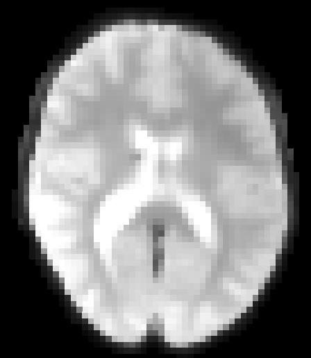
28 A simple experiment: the FFA Ss: 1 participant Design: 16s Faces, 16s Houses (block design) ake Voxel 15,19,18, in right posterior temporal cortex. Does this voxel care about faces?

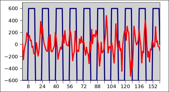
29 Model I: Boxcar Regressor Y = X *β

30 Model I: Boxcar Regressor

31 Model I: Boxcar Regressor 1 X X X Y t df = 2 1 X X t 159 = =

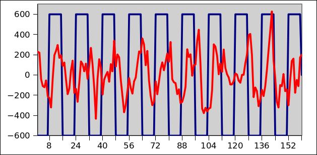
32 Model II: Convolved Boxcar Regressor Gaussian 1 X X X Y t df = 2 1 X X t 159 = =

33 Model II: Convolved Boxcar Regressor Gamma 1 X X X Y t df = 2 1 X X t 159 = =

34 Model II: Convolved Boxcar Regressor Double Gamma 1 X X X Y t df = 2 1 X X t 159 = =

35 What Convolution? Linear ime Invariant Basis Functions: Canonical HRF Canonical HRF + temp & disp derivs Informed basis set FIR/Smooth FIR Non Linear: Inverse Logit Balloon model

36 Canonical HRF Stimulus HRF (DGamma)

37 HRF Variability Across Subjects Handwerker et al 2004 Aguirre et Al 1998

38 HRF Variability Within Subjects same subject, same session same subject, different session Aguirre et al 1998

39 HRF Variability Across Brain Area Handwerker et al 2004 Handwerker et al 2004

40 Basis Functions I: HRF + Derivatives Canonical HRF emporal derivative Dispersion derivative

41 Basis Functions II: Fourier Basis Set f(t) h1(t) h2(t) h3(t)

42 Basis Functions III: Informed Basis Functions (FLOBS)

43 Basis Functions IV: FIR

44 Non Linear Approaches Model all 3 parameters (,W,H)

45 Slide from M Lindquist Inverse Logit Model Superposition of three inverse logit (sigmoid) functions. x 1 L x = 1 e Each function has three variable parameters dictating the amplitude, position and slope. h t θ =α 1 L t 1 / D 1 α 2 L t 2 / D2 α 3 L t 3 / D3 Lindquist & Wager (2007)

46 Slide from M Lindquist Flexibility By shifting the position of the second IL function one can model differences in duration. By shifting the position of all three IL functions one can model differences in onset.

47 Balloon Model BOLD response, % positive BOLD response initial overshoot dip post stimulus undershoot 0 stimulus time

48 What Convolution? - Recap he problem: Bias/Variance trade off Assume known shape v estimate X-Matrix mis-specification: Incorrect HRF will increase σ2

49 What Convolution? - Recap Canonical HRF: Pros: 1 parameter only, easy to interpret; easy to integrate at the second level. Cons: Bias in favour of a specific filter Basis Sets Functions: Pros: Flexible, can capture greater variability, unexpected and subject specific differences. Cons: many parameters to estimate (degrading dfs); difficult to interpret; how to aggregate at the 2nd level? Non-Linear Systems: Potentially very flexible and may better capture parameters and vasculature Computationally very demanding, parameters not obvious to interpret and aggregate across subjects (e.g., balloon model)

50 X-Matrix Assumptions Deterministic & known No regressor is a linear transformation of one (or more) regressors

51 Multicollinearity No column of the X matrix can be obtained by linear combination of one or more other columns. he issue is not whether there is/isn't multicollinearity, but rather, how much is there. wo main consequences: Decreased efficiency of the design degrades power. Parameter estimates can vary wildly, even in the wrong direction!

52 Source: J Mumford

53 Source: J Mumford

54 Source: J Mumford

55 Source: J Mumford

56 Source: J Mumford

57 Contrasts

58 Contrasts Cond A D A Cond B D B

59 Contrasts t= Var = 4. p Cond A D A Cond B D B

60 Contrasts t= Var = 4. p Cond A D A Cond B D B

61 Contrasts t= Var = 4. p Cond A D A Cond B D B

62 Contrasts t= Var = 4. p Cond A D A Cond B D B

63 Contrasts c t= Var c = 4. p c1 c2 c3 c= c4. cp Cond A D A Cond B D B

64 Contrasts c t= Var c = 4. p c= 0. 0 Cond A D A Cond B D B

65 Contrasts c t= Var c = 4. p c= 0. 0 Cond A D A Cond B D B

66 Contrasts c t= Var c = 4. p c= 0. 0 Cond A D A Cond B D B

67 Contrasts c t= Var c = 4. p c= 0. 0 Cond A D A Cond B D B

68 Contrasts c t= Var c

69 Model I: Boxcar Regressor 1 X X X Y t df = 2 1 X X t 159 = =

70 Model II: Convolved Boxcar Regressor Double Gamma 1 X X X Y t df = 2 1 X X t 159 = =

71 Gauss Markov Assumptions Under the following assumptions, the OLS estimator is the Best Linear Unbiased Estimator (BLUE). E i =0 Error has mean 0 Error is Homoschedastic i.i.d. 2 ~ N 0, I Var i = 2 Errors have same variance Errors are not Autocorrelated Cov i, j =0 Errors are independent of each other

72 emporal Structure If residuals are correlated, estimator is still unbiased but the variance estimate is not; and df are less than nominal. Corr(εt,εt-1) > 0 Corr(εt,εt-1) < 0

73 emporal Structure If residuals are correlated, estimator is still unbiased but the variance estimate is not; and df are less than nominal. his can affect your -test either way: i. Positive autocorrelation: underestimate of variance, -tests artificially inflated (actual α up to 0.16 for a nominal of 0.05). ii.negative autocorrelation: overestimate of variance, -test artificially reduced. wo strategies: i. High Pass filtering ii.autocorrelation correction ( pre-whitening ; colouring )

74 Low frequency noise Plenty low frequency noise: scanner drift, physiological (e.g., basal metabolism), psychological (e.g., learning, alertness changes), left-over from motion correction,... power spectrum noise signal power spectrum

75 HP Filtering Strategy I: SPM Model low drifts to soak up their variance (using a discrete cosine transform basis set).

76 HP Filtering Strategy II: FSL Remove low drifts from the signal: i. Fit a Gaussian-weighted running line

77 HP Filtering Strategy II: FSL Remove low drifts from the signal: i. Fit a Gaussian-weighted running line ii.subtract from data (red is pre-hpf, green is post-hpf)

78 Model II: Convolved Boxcar Regressor Double Gamma 1 X X X Y t df = 2 1 X X t 159 = =

79 Model III: High Pass Filter Double Gamma 1 X X X Y t df = 2 1 X X 349 t 159 = =

80 Autocorrelation GM Assumption: 2 i.i.d. ~ N 0, I Errors are independent of each other Cov i, j =0 fmri Data: i.i.d. 2 2 ~ N 0, V Cov i, j = V Y = X V Errors are NO independent of each other

81 Autocorrelation GM Assumption: i.i.d. 2 ~ N 0, I Cov i, j =0 cov(ε1,ε2) cov(ε2,ε1) cov(εn,ε1) cov(ε2,εn) Errors are independent of each other cov(ε1,εn) cov(ε2,εn)

82 Autocorrelation: Pre-whitening FSL If only we knew the structure of the serial correlation in the data (V) we could get rid of it: Given V, there exist a square (non singular) matrix K such that: i. V = KK ii. e = Kε (where ε is a 'well behaved' residual ~N(0,σ2I)) So, we can now clean-up (i.e., whiten ) our GLM 1 K Y =K X K Cov K = K V K = K KK K 2 = I

83 Autocorrelation: Pre-whitening FSL If only we knew the structure of the serial correlation in the data (V) we could get rid of it; but we don't know it. 1. Estimate the autocorrelation structure (for every voxel): Lag 1 [e01 e02 e03 e04 e05 e06 e07 e08 e09 e10 e11 e12] [e01 e02 e03 e04 e05 e06 e07 e08 e09 e10 e11 e12]

84 Autocorrelation: Pre-whitening FSL If only we knew the structure of the serial correlation in the data (V) we could get rid of it; but we don't know it. 1. Estimate the autocorrelation structure (for every voxel): Lag 2 [e01 e02 e03 e04 e05 e06 e07 e08 e09 e10 e11 e12] [e01 e02 e03 e04 e05 e06 e07 e08 e09 e10 e11 e12]

85 Autocorrelation: Pre-whitening FSL If only we knew the structure of the serial correlation in the data (V) we could get rid of it; but we don't know it. 1. Estimate the autocorrelation structure (for every voxel): Lag 3 [e01 e02 e03 e04 e05 e06 e07 e08 e09 e10 e11 e12] [e01 e02 e03 e04 e05 e06 e07 e08 e09 e10 e11 e

86 Autocorrelation: Pre-whitening FSL If only we knew the structure of the serial correlation in the data (V) we could get rid of it; but we don't know it. 1. Estimate the autocorrelation structure (for every voxel): Lag 8 [e01 e02 e03 e04 e05 e06 e07 e08 e09 e10 e11 e12] [e01 e02 e03 e04 e05 e06

87 Autocorrelation: Pre-whitening FSL If only we knew the structure of the serial correlation in the data (V) we could get rid of it; but we don't know it. 1. Estimate the autocorrelation structure (for every voxel): Lag 9 [e01 e02 e03 e04 e05 e06 e07 e08 e09 e10 e11 e12] [e01 e02 e03 e04 e05 e

88 Autocorrelation: Pre-whitening FSL If only we knew the structure of the serial correlation in the data (V) we could get rid of it; but we don't know it. 1. Estimate the autocorrelation structure (for every voxel) 2. For each lag, smooth estimates spatially ('regularization')

89 Autocorrelation: Pre-whitening FSL If only we knew the structure of the serial correlation in the data (V) we could get rid of it; but we don't know it. 1. Estimate the autocorrelation structure (for every voxel) 2. For each lag, smooth estimates spatially ('regularization') 3. Smooth (temporally) the correlation estimate, for each voxel ('ukey taper'). Woolrich et al, 2001 NeuroImage

90 Autocorrelation: Pre-whitening FSL If only we knew the structure of the serial correlation in the data (V) we could get rid of it; but we don't know it. 1. Estimate the autocorrelation structure (for every voxel) 2. For each lag, smooth estimates spatially ('regularization') 3. Smooth (temporally) the correlation estimate, for each voxel ('ukey taper'). Raw (rxx) Woolrich et al, 2001 NeuroImage Smooth (ρxx)

91 Autocorrelation: Pre-whitening FSL If only we knew the structure of the serial correlation in the data (V) we could get rid of it; but we don't know it. Now that we have an estimate of the structure, we can run a second regression in which we whiten the residuals using the estimated V. he estimated β for the new model are BLUE (under the assumption that V was appropriately modelled)

92 Autocorrelation: pre-whitening SPM Global estimation of the correlations: the correlation of the time series is averaged over voxels. Imposed AR(1) model with correlation 0.2 plus white noise.

93 Model III: High Pass Filter Double Gamma 1 X X X Y t df = 2 1 X X 349 t 159 = =

94 Model IV: Whitening Double Gamma 1 X X X Y t df = 2 1 X X t 159 = =

95 Whitening algorithms performance Lenoski 08 IEEE

96 Autocorrelation: Coloring i.i.d. 2 2 ~ N 0, V Cov i, j = V Y = X V Errors are NO independent of each other Impose a known correlation structure S If indeed SVS ~ SS then the error is N(0, σ2s) So: SY = SXβ + Sε Estimates are unbiased but no longer efficient (according to how well V is swamped )

97 Coloring v. Whitening Design Power Spectrum Coloring Pre-whitening

98 omorrow Setting up group fmri models Jeanette your group model challenges and she may choose it to include in her workshop

99