Analysis of fmri Timeseries:

Transcription

1 1 Chapter 10 Analysis of fmri Timeseries: Linear Time-Invariant Models, Event-related fmri and Optimal Experimental Design Rik Henson The Wellcome Dept. of Imaging Neuroscience & Institute of Cognitive Neuroscience University College London Queen Square, London, UK WC1N 3BG Tel (44) Fax (44) Contents I II III IV V Introduction fmri Timeseries Event-related fmri Design Efficiency Example References

2 2 I. INTRODUCTION This chapter discusses issues specific to the analysis of fmri data. It extends the Generalized Linear Model (GLM) introduced in Chapter 7 to linear time-invariant (LTI) systems, in which the Blood Oxygentation Level Dependent (BOLD) signal is modelled by neuronal causes that are expressed via a haemodynamic response function (HRF). The first section introduces the concepts of temporal basis functions, temporal filtering of fmri data and models of temporal autocorrelation. The second section describes the application of these ideas to event-related models, including issues relating to the temporal resolution of fmri. The third section concerns the efficiency of fmri experimental designs, as a function of the interstimulus interval and ordering of stimulus types. The final section illustrates some of the concepts introduced in the preceding sections with an example dataset from a single-subject event-related fmri experiment. II. FMRI TIMESERIES Unlike PET scans, it is important to order fmri scans as a function of time, i.e. treat them as a timeseries. This is because the BOLD signal will tend to be correlated across successive scans, meaning that they can no longer be treated as independent samples. The main reason for this correlation is the fast acquisition time (T R ) for fmri (typically 2-4s, cf minutes for PET) relative to the duration of the BOLD response (at least 30s). Treating fmri data as timeseries also allows us to view statistical analyses in signal-processing terms. The GLM can be expressed as a function of time (Friston et al., 1994; cf. Equation [1] in Chapter 7): y(t) = x c (t) β c + ε(t) ε(t) ~ N(0,σ 2 Σ) [1] where the data y(t) comprise the fmri timeseries (each timepoint representing one scan), the the explanatory variables, x c (t), c=1..n c are now functions of time, β c are the N c (timeinvariant) parameters, and Σ is the noise autocorrelation (see Section IIC below). Though y(t)

3 3 and x c (t) are discrete (sampled) timeseries (normally represented by the vector y and design matrix X respectively), we initially treat the data and model in terms of continuous time. A. Stimulus, Neural and Haemodynamic Models, and Linear Time-Invariance An explanatory variable x(t) represents the predicted BOLD response arising from a neural cause u(t). These neural causes (e.g., the local field potentials of an ensemble of neurons) normally follow a sequence of experimental stimulation, s(t). In SPM99, a distinction is made between neural activity that is impulsive (an event ) and that which is sustained for several seconds after stimulation (an epoch ). Both can be specified in terms of their onsets, but differ in the form of the neural model. For i=1..n i experimental conditions, each consisting of j=1..n j onset times o ij, the stimulus model is: s i (t) = Σ j=1..nj α ij δ(t-o ij ) [2] where α ij is a scaling factor and δ(t) is the (Dirac) delta function. The vector a i over the N j replications of the ith condition corresponds to a parametric modulation of that condition (e.g, by behavioural data associated with each stimulus; see Section VB for an example). 1 Below we assume α ij is fixed at 1. For events, the neural activity u i (t) is equated with s i (t). For epochs, the neural activity, r(τ), is modelled by b=1..n b temporal basis functions, g b (τ): r(τ) = Σ b=1..nb β b g b (τ) [3] where τ indexes a finite peristimulus time (PST) over the epoch duration T E (and β b are parameters to be estimated). Some example epoch response functions are shown in Figure 1A. The simplest is a single boxcar or tophat function that assumes a constant level of neural activity during the epoch. This can be supplemented by a (mean-corrected) exponential decay (e.g, of form exp{-τ/(4t E )}) to capture adaptation effects within an epoch. 1 A polynomial expansion of α ij can be used to test for higher order (nonlinear) dependencies of neural activity on the parametric factor.

4 4 Other examples include a half-sine, sin(πτ/t E ), and a discrete cosine transform (DCT) set, g b (τ) = cos{(b-1)πτ/t E }. The latter can capture any shape of neural response up to frequency limit (N b -1)/2T E. The neural activity then becomes (from [2] and [3]): u i (t) = s i (t) r(τ) = Σ j=1..nj Σ b=1..nb β b g b (t-o ij ) If we assume that the BOLD signal is the output of a linear time-invariant (LTI) system (Boynton et al., 1996) i.e. that the form of the response is independent of time, and the responses to successive stimuli superpose in a linear fashion then we can express x i (t) as the convolution of the neural activity with a haemodynamic response function (HRF), h(τ): x i (t) = u i (t) h(τ) [4] where τ now indexes a finite period, T H, over which the BOLD response lasts (a finite impulse response ). The HRF h(τ) is equivalent to the 1 st -order Volterra kernel (see Chapter 11). 2 Figure 1B shows the BOLD signal predicted from convolution of an epoch, modelled by box-car and exponential decay response functions, with a canonical form for the HRF. Also shown in Figure 1C is the BOLD signal predicted for a series of rapid events (delta functions); note the near-equivalent BOLD signal obtained 3 (provided the interevent interval is a few seconds or less). In other situations, we may not want to assume a fixed form for the HRF. Instead, we can allow for variability in its form by another expansion in terms of temporal basis functions, f k (τ): h(τ) = Σ k=1..nk β k f k (τ) [5] 2 It is also possible to model nonlinearites in the mapping from stimulus to neural activity in terms of a Volterra expansion (Josephs & Henson, 1999). However, because we normally only know the stimulus function (input) and the BOLD signal (output), we cannot attribute nonlinearites uniquely to the stimulus-to-neural or neural-to- BOLD (or bloodflow-to-bold) mappings. 3 bar a small shift in latency (Mechelli et al, in press-b)

5 5 (see Section IIIC for some examples). For a sequence of events, the GLM then becomes (from [1], [2] and [4]): y(t) = Σ i=1..ni Σ j=1..nj Σ k=1..nk β ijk f k (t-o ij ) + ε(t) where β ijk are the parameters to be estimated. In practice, the above models are simulated in discrete time. Nonetheless, given that significant information may exist in the predicted signal at frequencies above that associated with typical T R s, the simulations are performed in a timespace with multiple (T>1) timepoints per scan (i.e., with resolution, dt=t R /T seconds). This means, for example, that events do not need to be synchronised with scans (their onsets can be specified in fractions of scans). The high resolution timespace also ensures that a sequence of delta-functions (every dt seconds) becomes an adequate discrete-time approximation to a continuous boxcar function. To create the explanatory vectors, x c, in units of scans, the predicted BOLD signal is downsampled every T R (at a specified timepoint T0; Figure 2). In the general case, the number of columns in the design matrix will be N c =N i N j N k N b. B. Highpass Filtering We can also view the frequency components of our timeseries y(t) via the Fourier transform. A schematic of the power spectrum (the modulus of the complex Fourier components), typical of a subject at rest in the scanner, is shown in Figure 3A. This noise spectrum is dominated by low-frequencies, and has been characterised by a 1/f form when expressed in amplitude (Zarahn et al., 1997). The noise arises from physical sources, sometimes referred to as scanner drift (e.g., slowly-varying changes in ambient temperature), from physiological sources (e.g., biorhythms, such as ~1Hz respiratory or ~0.25Hz cardiac cycles, that are aliased by the slower sampling rate), and from residual movement effects and their interaction with the static magnetic field (Turner et al., 1998). When the subject is performing a task, signal components are added that we wish to distinguish from this noise. Figure 3B, for example, shows the approximate signal spectrum imposed by an (infinite) squarewave stimulation of 32s-on/32s-off. When averaging over all frequencies, this signal might be difficult to detect against the background noise. However, by filtering the data with an appropriate highpass filter (Figure 3C), we can remove most of the noise. Ideally, the

6 6 remaining noise spectrum would be flat (i.e., white noise, with equal power at all frequencies, though see Section IIC). The choice of the highpass cut-off would ideally maximise the signal:noise ratio. However, we cannot distinguish signal from noise on the basis of the power spectrum of the data alone. One choice of cut-off is to minimise the loss of signal, the frequency components of which are inherent in the design matrix X. SPM99 will offer such a cut-off by default (based on twice the maximum interval between the most frequently occurring condition). However, if this cut-off period is too great, the gain in signal passed can be outweighed by the extra noise passed. Thus some loss of signal may be necessary to minimise noise 4. Experimental designs should therefore not embody significant power at low frequencies (i.e, conditions to be contrasted should not live too far apart in time; see Section IVA). In the time domain, a highpass filter can be implemented by a DCT with harmonic periods up to the cut-off. These basis functions can be made explicit as confounds in the design matrix; or they can be viewed as part of a temporal smoothing matrix, S (together with any lowpass filtering; Section IIC). 5 This matrix is applied to both data and model: Sy = SXb + Se e ~ N(0,σ 2 V) V=SS S T (treating the timeseries as vectors), with the classical correction for the degrees of freedom lost in the filtering inherent in the equation for the effective df s (Chapter 9): v = trace{rv} 2 /trace{rvrv} R = I SX(SX) + [6] The effect of applying a highpass filter to real data (taken from a 42s epoch experiment; is illustrated in Figure 3D. Figure 3E shows the fitted responses after the filter S is applied to two boxcar models, one with and one without convolution with the HRF. The importance of convolving the neural model with an HRF is evident in the residuals (Figure 3F). Had the explanatory variables been directly equated with the stimulus function, significant temporal structure 4 In our experience, the 1/f noise becomes appreciable at frequencies below approximately 1/120 Hz, though this figure may vary considerably across scanners and subjects. 5 Though the matrix form expediates mathematical analysis, in practice highpass filtering is implemented by the computationally efficient subtraction of RR T y, where R is the residual-forming matrix associated with the DCT.

7 7 would remain in the residuals (e.g, as negative deviations at the start of each block, i.e, at higher frequency harmonics of the boxcar function). C Temporal Autocorrelation There are various reasons why the noise component may not be white even after highpass filtering. These include unmodelled neuronal noise sources that have their own haemodynamic correlates. Because these components live in the same frequency range as the effects of interest, they cannot be removed by the highpass filter. These noise sources induce temporal correlation between the residual errors, ε(t). Such autocorrelation is a special case of nonsphericity, which is treated more generally in Chapter 9. Here, we briefly review the various solutions to the specific problem of temporal autocorrelation in fmri timeseries. One solution proposed by Worsley and Friston (1995) is to apply a temporal smoothing. This is equivalent to adding a lowpass filter component to S (such that S, together with the highpass filter, becomes a bandpass filter). If the time-constants of the smoothing kernel are sufficiently large, the temporal autocorrelation induced by the smoothing can be assumed to swamp any intrinsic autocorrelation, S, such that: V = SS S T ~ SS T and thus the effective degrees of freedom can be calculated (via Equation [6]) solely via the known smoothing matrix. Lowpass filters derived from a Gaussian smoothing kernel with FWHM of 4-6s, or derived from a typical HRF, have been suggested (Friston et al., 2000b). An alternative solution is to estimate the intrinsic autocorrelation directly, which can be used to create a filter to pre-whiten the data before fitting the GLM. In other words, the smoothing matrix is set to S = K -1, where KK T is the estimated autocorrelation matrix. If the estimation is exact, then: V = K -1 S (K -1 ) T = K -1 KK T (K -1 ) T = I Two methods for estimating the autocorrelation are an autoregressive (AR) model (Bullmore et al, 1996) and a 1/f model (Zarahn et al., 1997). An AR(p) is a pth-order autoregressive model, having the time domain form:

8 8 z(t) = a 1 z(t-1) + a 2 z(t-2) + a p z(t-p) + w => z = Az + w w ~ N(0,σ 2 I) where A is a (p+1)x(p+1) lower-triangular matrix of regression coefficients, a i, that can be estimated by ordinary least-squares. Several authors (e.g, Bullmore et al, 1996; Kruggel & von Cramon, 1999) use an AR(1) model, in which the autocorrelation (a 1 ) and noise (σ 2 ) parameters are estimated from the residuals (z=e ) after fitting the GLM. These estimates are then used to create the filter S=(I-A) -1 that is applied to the data before re-fitting the GLM (a procedure that can be iterated until the residuals are white). The 1/f model is a linear model with the frequency domain form: g(f) = b 1 /f + b 2 p(f)=g(f) 2 where p(f) is the power spectrum, the parameters of which, b i, can be estimated from the Fourier-transformed data. The advantage of these methods is that they produce the most efficient estimation of the GLM parameters under Gaussian assumptions (corresponding to Gauss-Markov or minimum variance estimators ; Chapter 7). Temporal smoothing is generally less efficient because it removes high frequency components, which may contain signal. The disadvantage of the temporal autocorrelation models is that they can produce biased parameter estimates if the autocorrelation is not estimated accurately (i.e, do not necessarily produce minimum bias estimators ). Friston et al. (2000b) argued that the AR(1) and 1/f models are not sufficient to estimate the typical autocorrelation in fmri data. This is illustrated in Figure 4A, which shows the power spectra and autocorrelation functions 6 for the residuals of an event-related dataset (that in Section V). It can be seen that the AR(1) model underpredicts the intermediate-range correlations, whereas the 1/f model overpredicts the long-range correlations. Such a mismatch between the assumed (KK) and intrinsic (S ) autocorrelation 6 An autocorrelation function plots the correlation, ρ(t), as a function of lag, t=0 n-1, and is simply the Fourier transform of the power spectrum, p(f), where f=2πi, i=1..n-1.

9 9 will bias the statistics resulting from pre-whitening the data. 7 This mismatch can be ameliorated by combining bandpass filtering (Figure 4B) with modelling of the autocorrelation, in which case both models provide a reasonable fit (Figure 4C). Indeed, highpass filtering alone (with an appropriate cutoff) is normally sufficient to allow either model to fit the remaining autocorrelation (Friston et al, 2000b). SPM99 offers both an AR(1) model and lowpass smoothing as options (in conjunction with highpass filtering). The AR(1) model parameters are estimated from the data covariance, rather than the residuals. This removes the potential bias resulting from correlation in the residuals induced by removing modelled effects (Friston et al., 2002) 8, though it introduces potential bias resulting from signal and drifts in the data. The latter is ameliorated by pooling over voxels in the estimation of the AR(1) parameters, since only a minority of voxels typically contain signal. Another potential problem arises however if the temporal autocorrelation varies over voxels (Zarahn et al., 1997). For example, it has been argued to be higher in grey than white matter (Woolrich et al., 2001). This can be accommodated by estimating voxel-specific AR(p) parameters (possibly together with some spatial regularisation, Worsley et al, 2002), though it means that different voxels can have different effective degrees of freedom, which in strict terms violates the assumptions behind Gaussian Field Theory (Chapters 14-15). Such spatial variation is less of a problem for the temporal smoothing approach, which homogenises the autocorrelation across voxels. A final problem with the above methods is that the model parameters and autocorrelation parameters are estimated separately, which requires multiple passes through the data and makes it difficult to properly accommodate the associated degrees of freedom. Iterative estimation schemes, such as Restricted Maximum Likelihood (ReML), allow simultaneous estimation of model parameters and autocorrelation (hyper)parameters, together with proper partitioning of the effective degrees of freedom (see Chapter 9 for more details). This method can be used with any temporal autocorrelation model. Friston et al. (2002) chose an AR(1)+white noise model: y = Xb + z 1 + z 2 z 1 = Az 1 + w w=n(0,σ 1 2 I) z 2 =N(0,σ 2 2 I) 7 More complex models of the temporal autocorrelation have since been shown to minimise bias, such as Tukey tapers (Woolrich et al., 2001) and autoregessive moving average (ARMA) models, a special case of the latter being an AR(1)+white noise model (Burock & Dale, 2000; see below). 8 though there are ways of reducing this bias (Worsely et al, 2002)

10 10 for which the autocorrelation coefficient a 1 was fixed to exp(-1), leaving two hyperparameters (σ 2 1 and σ 2 2 ). The additional white-noise component (z 2 ) contributes to the zero-lag autocorrelation, which in turn allows the AR(1) model to capture better the shape of the autocorrelation for longer lags. Note that this approach still requires a highpass filter to provide accurate fits (Figure 4D), though a subtle difference from the above residual-based approaches is that the highpass filter is also treated as part of the complete model to be estimated, rather than a pre-whitening filter. Such iterative schemes are computationally expensive when performed at every voxel. One possible solution is to assume that the ratio of hyperparameters is stationary over voxels, which allows the data to be pooled over voxels in order to estimate this ratio. Spatial variability in the absolute autocorrelation can be accommodated by subsequently estimating a single voxel-specific scaling factor (see Friston et al, 2002, and Chapter 9 for further details). This scaling factor can be estimated in one-step (since no iteration is required for ReML to estimate a single hyperparameter). This ReML solution to modelling the autocorrelation therefore shares the efficiency of pre-whitening approaches, though with less potential bias, allows proper adjustment of the degrees of freedom, and makes some allowance for spatial variability in the temporal autocorrelation. This obviates the need for temporal smoothing, a consequence particularly important for event-related designs (below), in which appreciable signal can exist at high frequencies that would be lost by lowpass smoothing (see Figure 4D). This approach has been implemented in SPM2. III. EVENT-RELATED FMRI Event-related fmri (efmri) is simply the use of fmri to detect responses to individual trials, in a manner analogous to the time-locked event-related potentials (ERPs) recorded with EEG. The neural activity associated with each trial is normally (though not necessarily) modelled as a delta function an event at the trial onset. A. Advantages of efmri The advent of event-related methods offers several advantages for experimental design. Foremost is the ability to intermix trials of different types (conditions), rather than blocking

11 11 them in the manner required for PET and initially adopted for fmri (cf. Figures 5A and 5B). The counterbalancing or randomising of different trial-types, as is standard in behavioural or electrophysiological studies, ensures that the average response to a trial-type is not biased by a specific context or history of preceding trial-types. This is important because the (unbalanced) blocking of trial-types might, for example, induce differences in the cognitive set or strategies adopted by subjects. This means that any difference in the mean activity during different blocks might reflect such state effects, rather than item effects specific to individual trials (e.g., Rugg & Henson, 2002). Johnson et al. (1997) for example, provided direct evidence that the presentation format intermixed or blocked can effect the ERP associated with a trial-based memory effect. 9 A second advantage of event-related methods is that they allow categorisation of trialtypes according to the subject s behaviour. This might include separate modelling of trials with correct and incorrect task performance, or parametric modelling of trial-by-trial reaction times (modulations that are only possible indirectly when analysed at a block level). An appealing example of this facility occurs in subsequent memory experiments. In such experiments, subjects perform a simple study task on a series of items, followed by a surprise memory test. The latter allows the items in the study task to be categorised according to whether they were later remembered (a categorisation the researcher has little objective control over). Brain regions can then be isolated whose activity predicts subsequent memory (e.g., Henson et al., 1999). A third advantage reflects the identification of events whose occurrence can only be indicated by the subject. An example of such an event is the spontaneous transition between the perception of ambiguous visual objects, as in the face-vase illusion (Kleinschmidt et al., 1998), or between 2D and 3D perception of 2D stereograms (Portas et al., 2000); situations where the objective stimulation is constant. A fourth advantage is that event-related methods allow some experimental designs that cannot be easily blocked. One example is an oddball design, in which the stimulus of interest is one that deviates from the prevailing context, and therefore cannot be blocked by definition (Strange et al., 2000). 9 Note that there are also disadvantages associated with randomised designs. Foremost, such designs are generally less efficient for detecting effects than blocked designs (with short SOAs and reasonable block lengths; see section IVA below). In addition, some psychological manipulations, such as changes in selective attention or task, may exert stronger effects when blocked.

12 12 A final advantage is that event-related methods potentially allow more accurate models of the data. Even when trial-types are blocked, for example, modelling the BOLD response to each trial within a block may capture additional variability that is not captured by a simple box-car neuronal model, particularly for intertrial intervals of more than a few seconds (Price et al., 1999; cf. Figures 5A and 5C). Furthermore, it is possible distinguish between state effects and item effects. Chawla et al. (1999), for example, investigated the interaction between selective attention (a state effect) and transient stimulus changes (an item effect) in a mixed epoch/event design. Subjects viewed a visual stimulus that occasionally changed in either colour or motion. In some blocks, they were required to detect the colour changes; in other blocks they detected the motion changes. By varying the interval between changes within a block, Chawla et al. were able to reduce the correlation between the corresponding epoch- and event-related regressors. Tests of the epoch-related effect showed that attending towards a specific visual attribute (e.g. colour) increased the baseline activity in regions selective for that attribute (e.g. V4). Tests of the event-related effect showed that the impulse response to the same objective change in visual attribute was augmented when subjects were attending to that attribute. These combined effects of selective attention raising endogenous baseline activity and increasing the gain of the exogenous response could not be distinguished in blocked designs (Figure 5D). B. The BOLD impulse response A typical BOLD response to an impulse stimulation (event) is shown in Figure 6A. The response peaks approximately 5 seconds after stimulation, and is followed by an undershoot that lasts approximately 30 seconds (at high magnetic fields, an initial undershoot can sometimes be observed, Malonek & Ginvald, 1996). Early event-related studies therefore used a long interstimulus interval (or more generally, Stimulus Onset Asynchrony, SOA, when the stimuli are not treated as delta functions) to allow the response to return to baseline between stimulations. However, although the responses to successive events will overlap at shorter SOAs, this overlap can be explicitly modelled (via an HRF). This modelling is simplified if successive responses can be assumed to add in a linear fashion (Section IA). Short SOAs of a few seconds are desirable because they are comparable to those typically used in behavioural and electrophysiological studies, and because they are generally more efficient from the statistical perspective (Section IVA).

13 13 There is good evidence for nonlinearity in the BOLD impulse response as a function of SOA (Friston et al., 1998a; Miezin et al., 2000; Pollman et al., 1997). 10 This nonlinearity is typically a saturation whereby the response to a run of events is smaller than would be predicted by the summation of responses to each event alone. This saturation is believed to arise in the mapping from bloodflow to BOLD signal (Friston et al., 2000a), though may also have a neural locus, particularly for very short SOAs (for biophysical models that such incorporate nonlinearities, see Chapter 11). It has been found for SOAs below approximately 8s, and the degree of saturation increases as the SOA decreases. For typical SOAs of 2-4s however, its magnitude is small (typically less than 20%, Miezin et al., 2000). Note that the dominant effect of increasing the duration of neural activity (up to 2-4 seconds) in a linear-convolution model (Equation [4]) is to increase the peak amplitude of the BOLD response (Figure 6B). In other words, the BOLD response integrates neural activity over a few seconds. This is convenient because it means that neural activity can be reasonably modelled as a delta function (i.e., even though the amplitude of the response may vary nonlinearly with stimulus duration, Vasquez & Noll, 1998, the shape of the response does not necessarily change dramatically). The corollary however is that a difference in the amplitude of the BOLD impulse response (as conventionally tested) does not imply a difference in the mean level of neural activity: the difference could reflect different durations of neural activity at same mean level. One way to tease these apart is to test for subtle differences in the peak latency of the BOLD impulse response (Section IIF below), which will differ in the latter case but not former case (Figure 5C). The general shape of the BOLD impulse response appears similar across early sensory regions, such as V1 (Boynton et al., 1996), A1 (Josephs et al., 1997) and S1 (Zarahn et al., 1997). However, the precise shape has been shown to vary across the brain, particularly higher cortical regions (Schacter et al., 1997), presumably due mainly to variations in the vasculature of different regions (Lee et al., 1995). Moreover, the BOLD response appears to vary considerably across people (Aguirre et al., 1998). 11 These types of 10 Nonlinearites in the amplitude of the BOLD response are also found as a function of stimulus duration or stimulus magnitude (Vasquez & Noll, 1998). Nonlinearities also appear to vary considerably across different brain regions (Huettel & McCarthy, 2001; Birn et al. 2001). 11 One possible solution is use subject-specific HRFs derived from a reference region known to respond to a simple task (e.g, from central sulcus during a simple manual task performed during a pilot scan on each subject,

14 14 variability can be accommodated by expanding the HRF in terms of temporal basis functions (Equation [5]). C. Temporal Basis Functions Several temporal basis sets are offered in SPM. The most general are the Finite Impulse Response (FIR) and Fourier basis sets, which make minimal assumptions about the shape of the response. The FIR set consists of N k contiguous box-car functions of PST, each of duration T H /N k seconds (Figure 7A), where T H is the maximum duration of the HRF. The Fourier set (Figure 7B) consists of N s sine and N s cosine functions of harmonic periods T H, T H /2 T H /N s, (i.e., N k =2N s +1 basis functions, where the last is the mean of the basis functions over T H ). 12 Linear combinations of the (orthonormal) FIR or Fourier basis functions can capture any shape of response up to a specified timescale (T H /N k in the case of the FIR) or frequency (N s /T H in the case of the Fourier set). 13 In practice, there is little to choose between the FIR and Fourier sets: The Fourier set may be better suited when the PST sampling is non-uniform (Section IIE); whereas the parameter estimates for the FIR functions have a more direct interpretation in terms of averaged PST signal (effecting a linear deconvolution ). Indeed, in the special case when T H /N k =T R, the FIR functions are delta functions: h(τ) = Σ k=1..nk δ(τ-k-1) over the N k poststimulus scans, and the design matrix for events onsetting at scan o ij is: x tc = Σ i=1..ni Σ j=1..nj Σ k=1..nk δ(t-(o ij +k-1)) Aguirre et al, 1998). However, while this allows for inter-subject variability, it does not allow for inter-regional variability within subjects (or potential error in estimation of the reference response, Friston et al., 2002). 12 Since the HRF is assumed to be bounded at zero for τ<=0 and τ>=t H, the Fourier basis functions can also be windowed (e.g, by a Hanning window) within this range. 13 In practice, there is little point in making T H /N k smaller than the effective PST sampling interval, T s, (Section IIE) or specifying N s /T H higher than the Nyquist limit 1/(2T s ).

15 15 where t indexes scans and c indexes the column for the kth basis function of the jth event of the ith type (Ollinger et al., 2001; see Figure 16A, for an example). For the special case of non-overlapping responses (i.e., that o ij +k o uv +w for all i u, j v and k w), the estimates β ik of the FIR parameters are equivalent to the simple trial-averaged data: β ik = Σ j=1..nj y(o ij +k-1) / N j This estimation also approximates the HRF when the event-types are fully counterbalanced (such that the number of occasions when o ij +k = o uv +w is constant for all i u, j v and k w, which is approached when events are randomised and N j is large 14 ), a procedure that has been called selective averaging (Dale & Buckner, 1997). It is equivalent to noting that the covariance matrix X T X (sometimes called the overlap correction matrix, Dale, 1999) approaches the identity matrix (after mean-correction), such that the ordinary least-squares estimates become: b = (X T X) 1 X T y X T y Note that such counterbalancing is not required by the full pseudoinverse estimation used by SPM (though there may still be important psychological reasons for counterbalancing). More parsimonious basis sets can be chosen that make various assumptions about the shape of the HRF. 15 One popular choice is the gamma function: f(τ) = ((τ-o)/d) (p-1) e -(τ-o)/d / (d(p-1)!) [7] where o is the onset delay, d is the time-scaling, and p is an integer phase delay (the peak delay is given by pd, and the dispersion by pd 2 ). The gamma function has been shown to provide a reasonably good fit to the impulse response (Boynton et al., 1996), though it lacks an undershoot (Fransson et al., 1999; Glover, 1999). The first T H seconds of a set of N k 14 In strict terms, this also means an equal number of occasions (scans) when event-types co-occur (i.e are conincident), which is not normally the case. 15 Unlike the Fourier or FIR sets, this set is not strictly a basis set in that it does not span the space of possible responses within the response window T H, but we maintain the term here for convenience.

16 16 gamma functions of increasing dispersions can be obtained by incrementing p=2..n k +1 (Figure 7C), which can be orthogonalised with respect to one another (as in SPM). This set is more parsimonious in that fewer functions are required to capture the typical range of impulse responses than are required by the Fourier or FIR sets, reducing the degrees of freedom used in the design matrix and allowing more powerful statistical tests. An even more parsimonious basis set, suggested by Friston et al. (1998), is based on a canonical HRF and its partial derivatives (Figure 7D). The canonical HRF is a typical BOLD impulse response characterised by two gamma functions, one modelling the peak and one modelling the undershoot. The canonical HRF is parameterised by an onset delay of 0s, peak delay of 6s, peak dispersion of 1, undershoot delay of 16s, undershoot dispersion of 1 and a peak:undershoot amplitude ratio of 6; values that were derived from a principal component analysis of the data reported in Friston et al. (1998a). To allow for variations about the canonical form, the partial derivatives of the canonical HRF with respect to, for example, its peak delay and dispersion parameters can be added as further basis functions. By a first-order multivariate Taylor expansion (cf. Equation [8] below), the temporal derivative can capture differences in the latency of the peak response, while the dispersion derivative can capture differences in the duration of the peak response. 16 D. Statistical Tests of Event-related Responses, and Which Basis Set? Inferences using multiple basis functions are generally made with F-contrasts (Chapter 8). An example F-contrast that tests for any difference in the event-related response to two trialtypes modelled by an FIR set is shown in Figure 16B. Further assumptions about the shape of the response (or nature of differences between responses) can also be entered at the contrast level (Burock & Dale, 2000; Henson et al., 2001a). One might restrict differential contrasts to a limited set of FIR time-bins for example. In the extreme case, setting the contrast weights for an FIR set to match an assumed HRF shape will produce a parameter estimate for the contrast proportional to that obtained by using that HRF as a single basis function (assuming that FIR timebins are sampled uniformly at each effective sampling interval). 16 A similar logic can be used to capture different latencies of epoch-related responses, viz. by adding the temporal derivatives of the (HRF-convolved) epoch response functions. Note that variations in the HRF can also be accommodated by nonlinear, iterative fitting techniques (Section IIIF; see Hinrichs et al, 2000, for a combination of nonlinear estimation of HRF shape together with linear deconvolution of responses).

17 17 However, when the real response resembles an assumed HRF, tests on a model using that HRF as a single basis function are more powerful (Ollinger et al., 2001). In such cases, t- tests on the parameter estimate for a canonical HRF for example can be interpreted in terms of the amplitude of the response. However, when the real response differs appreciably from the assumed form, tests on the HRF parameter estimates are biased (and unmodelled structure will exist in the residuals). In such cases, a canonical HRF parameter estimate can no longer necessarily be interpreted in terms of amplitude (see Chapter 8). The addition of partial derivatives of the HRF (see above) can ameliorate this problem: the inclusion of a temporal derivative for example can reduce the residual error by capturing systematic delays relative to the assumed HRF. 17 Nonetheless, for responses that differ by more than 1s in their peak latency (i.e, when the first-order Taylor approximation fails), different canonical HRF parameters will be estimated even when the responses have identical peak amplitudes. An important empirical question then becomes: How much variability exists around the canonical form? Henson et al. (2001b) addressed this question in a dataset involving rapid motor responses to brief presentations of faces across 12 subjects (the superset of the data in Section V). By modelling the event-related response with a canonical HRF, its partial derivatives and an FIR basis set, the authors assessed the contribution of the different basis functions by a series of F-contrasts. Significant variability was captured by both the temporal derivative and dispersion derivative, confirming that different regions exhibited different shaped responses. Little additional variability was captured by the FIR basis set however, suggesting that the canonical HRF and its two partial derivatives were sufficient to capture the majority of experimental variability (at least in regions that were activated in this task). This sufficiency may be specific to this dataset, and reflect the fact that neural activity was reasonably well modelled by a delta function. It is unlikely to hold for more complex experimental trials, such as working memory trials where information must be maintained for 17 Note that the inclusion of the partial derivatives of an HRF does not necessarily affect the parameter estimate for the HRF itself, since the basis functions are orthogonal (unless correlations between the regressors arise owing to under-sampling by the T R or by temporal correlations between the onsets of events of different types). In other words, their inclusion does not necessarily affect second-level t-tests on the HRF parameter estimates alone. Note also that t-tests on the partial derivatives are not meaningful in the absence of information about the HRF parameter estimate: the derivative estimates depend on the size (and sign) of the HRF estimate (Section IVF), and are unlikely to reflect plausible impulse responses (versus baseline) in the absence of a significant HRF parameter estimate.

18 18 several seconds (e.g, Ollinger et al., 2001). Nonetheless, such trials may be better accommodated by more complex neural models, expanding u(t) in terms of multiple events/epochs (cf. Equation [3]), while still assuming a fixed form for the HRF. This allows more direct inferences about stimulus, response and delay components of a trial for example (Zarahn, 2000). More generally, the question of which basis set to use becomes a problem of model selection (Chapter 7). A problem arises when one wishes to use multiple basis functions to make inferences in second-level analyses (e.g., in random effects analyses over subjects; see Chapter 12). Subject-specific beta images created after fitting an FIR model in a first-level analysis could, for example, enter into a second-level model as a peristimulus time factor (differential F-contrasts on which would correspond to a condition-by-time interaction in a conventional repeated-measures ANOVA). However, the parameter estimates are unlikely to be independent or identically-distributed over subjects, violating the sphericity assumption of univariate tests (Chapter 9). 18 One solution is to use multivariate tests (Henson, et al., 2000), though these are generally less powerful (by virtue of making minimal assumptions about the data covariance). The use of ReML or Parametric Empirical Bayes methods to estimate the hyper-parameters governing constraints placed on the covariance matrix (Friston et al., 2002; Chapter 9) resolves this problem. E. Timing Issues: Practical There are both practical and theoretical issues pertaining to the timing of BOLD responses. Two practical issues concern the effective sampling rate of the response and the different acquisition times for different slices (using EPI). It is possible to sample the impulse response at post-stimulus intervals, T s, shorter than the interscan interval T R by jittering event onsets with respect to scan onsets (Josephs et al. 1997). Jittering can be effected by ensuring the SOA is not a simple multiple of the T R, or by adding a random trial-by-trial delay in stimulus onsets relative to scan onsets (Figure 8). In both cases, different PSTs are sampled over trials (the main difference between the two methods being whether the SOA is fixed or random). For example, an effective PST 18 This is one reason why researchers have tended to stick with t-tests on (contrasts of) the parameter estimate for a single canonical HRF at the second-level, at the expense of generality (potentially missing responses with a non-canonical form).

19 19 sampling of 0.5Hz can be achieved with an SOA of 6s and a T R of 4s; or by adding a delay of 0 or 2s randomly to each trial (producing SOAs of 4-8s, with a mean of 6s). While effective sampling rates higher than the T R do not necessarily affect response detection for typical T R s of 2-4s (since there is little power in the canonical response above 0.2Hz; see Figure 6A), higher sampling rates are important for quantifying the response shape, such as its latency (Miezin et al, 2000; Section IVF). Jittering event onsets with respect to scan onsets does not help the second practical issue concerning different slice acquisition times. This slice-timing problem (Henson et al., 1999) refers to the fact that, with a descending EPI sequence for example, the bottom slice is acquired T R seconds later than the top slice. If a single basis function (such as a canonical HRF) were used to model the response, and onset times were specified relative to the start of each scan, the data in the bottom slice would be systematically delayed by T R seconds relative to the model. 19 This would produce poor (and biased) parameter estimates for later slices, and mean that different sensitivities would apply to different slices. 20 There are two main solutions to this problem: to interpolate the data in each slice as if the slices were acquired simultaneously, or use a basis set that allows for different response onset latencies. Temporal interpolation of the data (using a full sinc interpolation) is possible during preprocessing of images in SPM99. For sequential acquisition schemes, temporal interpolation is generally better when performed after spatial realignment, since the timing error for a voxel re-sliced to nearby slices will be small relative to the potential error for a voxel that represents different brain regions owing to interscan movement. (This may not be true for interleaved acquisition schemes, for which temporal interpolation might be better before spatial realignment). The data are interpolated by an amount proportional to their sampling time relative to a reference slice (whose data are unchanged). The event onsets can then be synchronised with the acquisition of the reference slice. In SPM, this is equivalent to maintaining event onsets relative to scan onsets, but setting the timepoint T0 in the simulated timespace of T time-bins (Section IIA), from which the regressors are sampled, to: 19 One solution would be to allow different event onsets for different slices. SPM however assumes the same model (i.e. onsets) for all voxels (i.e. slices) in order to equate the degrees of freedom (e.g. residual autocorrelation) across voxels required for GFT (Chapters 14-15). Moreover, slice-timing information is lost as soon as images are re-sliced relative to a different orientation (e.g. during spatial normalisation). 20 This is less of a problem for low-frequency responses, such as those induced by epochs of tens of seconds.

20 20 T0 = round{nt/ N s } where the reference slice is the nth slice acquired of the N s slices per scan. A problem with slice-timing correction is that the interpolation will alias frequencies above the Nyquist limit 1/(2T R ). Ironically, this means that the interpolation accuracy decreases as the slice-timing problem (ie T R ) increases. For short T R s < 2-3s, the interpolation error is likely to be small. For longer T R s, the severity of the interpolation error depends on whether appreciable signal power exists above the Nyquist limit (which is more likely for rapid, randomised event-related designs; see below). An alternative solution to the slice-timing problem is to include additional basis functions that can accommodate timing errors. The Fourier basis set for example does not have a slice-timing problem (i.e, it is phase-invariant). For more constrained sets, the addition of the temporal derivatives of the functions may be sufficient. The parameter estimates for the derivatives will vary across slices, to capture shifts in the data relative to the model, while those for the response functions can remain constant (up to a first-order Taylor approximation). The temporal derivative of the canonical HRF for example (Figure 7D) can accommodate slice-timing differences of approximately +/-1s (i.e, T R s of 2s, when the model is synchronised to the middle slice in time). A problem with this approach is that slicetiming differences are confounded with latency differences in the real response. This means that response latencies cannot be compared across different slices (see below). F. Timing Issues: Theoretical Assuming that the data are synchronised with the event onsets, there may be theoretical reasons for investigating aspects of the BOLD response latency (as well as its amplitude). For example, BOLD responses arising from blood vessels (e.g. veins) tend to have longer latencies than those from parenchyma (Saad et al., 2001). Though absolute differences in response latency across brain regions are unlikely to be informative regarding underlying neural activity, since they may simply reflect differences in vasculature 21, differences in the relative response latencies in different conditions may inform theories about the separate 21 Miezin et al (2000), for example, showed that the peak response in motor cortex preceded that in vis ual cortex for events in which the motor response succeeded visual stimulation.

21 21 stages of underlying neural processes. Latency estimates may also correlate better with some behavioural measures, such as reaction times (Kruggel et al., 2000). For periodic responses, latency can be estimated easily using Fourier (Rajapakse et al, 1998) or Hilbert (Saad et al. 2001) transforms. For nonperiodic responses, the simplest approach is to construct a measure of latency from the trial-averaged response, such as the linear intercept to the ascending region of the peak response (using a very short T R, Menon et al, 1998), or the peak of a spline interpolation through the data (Huettel & McCarthy, 2001). Other approaches estimate the latency directly from a parameterised HRF, using either linear or nonlinear (iterative) fitting techniques. A linear method for estimating latency within the GLM was proposed by Friston et al. (1998b). Using a first-order Taylor expansion of the response, these authors showed how the standard error of a fitted response can be estimated from the temporal derivative of an HRF. This approach was extended by Henson et al. (2002a) in order to estimate response latency directly. If the real response, r(τ), is a scaled (by α) version of an assumed HRF, h(τ), but shifted by a small amount dτ, then: r(τ) = α h(τ + dτ) α h(τ) + α h(τ) dτ [8] where h(τ) is the first derivative of h(τ) with respect to τ. If h(τ) and h(τ) are used as two basis functions in the GLM to estimate the parameters β 1 and β 2 respectively, then: β 1 = α β 2 = αdτ => dτ = β 2 / β 1 In other words, the latency shift can be estimated by the ratio of the derivative to HRF parameter estimates (a similar logic can be used for other parameters of the HRF, such as its dispersion). The first-order approximation holds when dτ is small relative to the timeconstants of the response (see Liao et al, 2002, for a more general treatment, using the first and second derivatives of a parameter representing the scaling of τ). When using SPM s canonical HRF and temporal derivative for example, the approximation is reasonable for latency of shifts of ±1s relative to the canonical HRF. Whole-brain SPMs of differences in

22 22 response latencies can be constructed simply by comparing the ratios (e.g, over subjects) of the temporal derivative to canonical HRF parameter estimates at every voxel (Figure 9A). 22 Other methods use nonlinear (iterative) fitting techniques. These approaches are more powerful (e.g., can capture any size latency shift), but computationally expensive (and hence often restricted to regions of interest). Various parameterisations of the HRF have been used, such as a Gaussian function parameterised by amplitude, onset latency and dispersion (Kruggel et al., 1999) or a gamma function parameterised by amplitude, onset latency and peak latency (Miezin et al., 2000). Henson & Rugg (2001) used SPM s canonical HRF with the amplitude, onset latency and peak latency parameters free to vary. 23 The latter was applied to a rapid event-related experiment in which an FIR basis set was used to first estimate the mean event-related response to first and second presentations of faces in a fusiform face area. A subsequent nonlinear fit of the canonical HRF to these deconvolved data revealed significant differences (over subjects) in the amplitude and peak latency parameters, but not in the onset latency parameter (Figure 9B). The most parsimonious explanation for this pattern is that repetition of a face decreased the duration of underlying neural activity (assuming a linear convolution model; see Figure 6C). A problem with unconstrained iterative fitting techniques is that the parameter estimates may not be optimal (because of local minima in the search space). Parameters that have correlated effects compound this problem (e.g., situations can arise in noisy data where the estimates of onset and peak latency take implausibly large values of opposite sign). One solution is to put priors on the likely parameter distributions in a Bayesian estimation scheme (Chapter 11) to regularise the solutions (see Gossl et al, 2001, for an example). IV. EFFICIENCY AND OPTIMISATION OF EXPERIMENTAL DESIGN This section is concerned with optimising experimental designs in order to detect particular effects. The aim is to minimise the standard error of a contrast, c T b (i.e. the denominator of a 22 To allow for voxels in which the approximation breaks down (e.g., for canonical HRF parameter estimates close to zero), Henson et al. (2002) applied a sigmoidal squashing function to constrain the ratio estimates. 23 The advantage of a Gaussian HRF is that its onset delay and dispersion are independent, unlike a gamma HRF (Equation [7]). A problem however is that a Gaussian HRF is not bounded for τ<0, and does not allow for the asymmetry typically found in the BOLD response. A problem with both a Gaussian HRF and a single

23 23 t-statistic, Chapter 8), given a contrast matrix c and parameter estimates b, whose variance is (Friston et al, 2000b): Var{c T b } = σ 2 c T (SX) + SVS T (SX) +T c [9] We want to minimise [9] with respect to the design matrix, X, assuming that the filter matrix S, noise autocorrelation matrix V and noise variance σ 2 are constant (though the autocorrelation and noise may in fact depend on the design; see below). If we incorporate S into X, and assume V=I, then this is equivalent to maximising the efficiency, e, of a contrast, defined by: e(c,x) = (σ 2 c T (X T X) -1 c) -1 [10] This equation can be split into the noise variance, σ 2, and the estimator variance, X T X (Mechelli et al., in press-a). 24 If one is interested in multiple contrasts, expressed in a matrix C, and assume σ 2 is constant, then the efficiency of a design can be defined as (Dale, 1999): e(x) trace{c T (X T X) -1 C} -1 [11] A. Single Event-type Designs For a single event-type, the space of possible experimental designs can be captured by two parameters: the minimal SOA (SOA m ) and the probability, p, of an event occurring at every SOA m (Friston et al, 1999a). In deterministic designs, p=1 every fixed multiple of SOA m, and p=0 otherwise (i.e. a series of events with fixed SOA; Figure 10A). In stochastic designs, 0<=p<=1 (producing a range of SOAs). For stationary stochastic designs, 0<p<1 is constant, giving an exponential distribution of SOAs; for dynamic stochastic designs, p is itself a function of time. The temporal modulation of p(t) in dynamic stochastic designs might be sinusoidal, for example, or a squarewave, corresponding to a blocked design. Also gamma HRF is that they do not allow for a post-peak undershoot. A problem with the double (canonical) gamma HRF used by Henson & Rugg (2001) is that the onset latency and peak latency are correlated. 24 Note that this measure of efficiency is not invariant to the scaling of the contrast vectors c, which should therefore be normalized.

24 24 shown in Figure 10A is the efficiency of each design (to detect a basic impulse response, i.e, C=[1], assuming a canonical HRF). For short SOA m, the blocked design is most efficient, and the deterministic design least efficient. For stochastic designs, efficiency is generally maximal when the SOA m is minimal and the (mean) p=0.5 (Friston et al, 1999a). Efficiency can also be considered in signal-processing terms (Josephs & Henson, 1999). In the frequency domain, the HRF can be viewed as a filter. The most efficient contrast is one that passes maximum neural signal power at the dominant frequency of the HRF. Since the dominant frequency of a canonical HRF is approximately 30s (Figure 6A), a blocked design with minimal SOA m (large power) and a cycling frequency close to this figure (e.g, 15s on; 15s off) is very efficient. (Indeed, the most efficient design in this case would be a continuous sinusoidal modulation of neural activity with period of 30s, corresponding to a delta function at 0.033Hz). The effect of bandpass filtering can also be viewed in these terms. Since the HRF and S matrix convolutions are commutative, a single equivalent filter can be calculated (the effective HRF, Josephs & Henson, 1999). Blocked designs with long cycling periods are undesirable since the majority of the induced variance is not passed by the highpass filter (i.e, will be indistinguishable from low-frequency noise). Deterministic single-event designs with a short SOA m will induce high frequency neural variance that is not passed by the HRF (or lowpass filter). Stochastic designs however induce variance over a range of frequencies, so can be reasonably efficient with a short SOA m. A distinction has been made between detection power and estimation efficiency (Liu et al, 2001; Birn et al, 2002). The former refers to the ability to detect a significant response; the latter refers to the ability to estimate the shape of the response. The above examples, which assume a canonical HRF, relate to detection power. The concept of estimation efficiency can be illustrated simply by considering a more general basis set, such as an FIR. Multiple parameters now need to be estimated (X has multiple columns, Figure 10B), and efficiency is maximal (Equation [11]) when the covariance between the columns of X is minimal. In this case (with contrast C=I), blocked designs are less efficient than randomised designs (Figure 10C, since the FIR regressors are highly correlated in blocked designs). This is the opposite of the situation with a single canonical HRF, for which blocked designs are more efficient than randomised designs. An alternative perspective is that the FIR basis functions have more high frequency components, and therefore pass more signal at the higher frequencies that arise from randomised designs (Figure 10D).

25 25 Thus the different considerations of detecting a response versus characterising the form of that response require different types of experimental design. Hagberg et al. (2001) considered a range of possible SOA distributions (bimodal in the case of blocked designs; exponential in the case of fully randomised designs) and showed that long-tail distributions combine reasonable detection power and estimation efficiency (though uniform distributions, such as those based on a Latin Square, did as well on empirical data). B. Multiple Event-type Designs For multiple event-types, the space of possible designs can be characterised by SOA m and a transition matrix (Josephs & Henson, 1999). For N i different event-types, a N m i by N i transition matrix captures the probability of an event being of each type, given the history of the last 1..m event-types (some examples are shown in Figure 11). A fully randomised design with two event-types (A and B) has a simple first-order transition matrix in which each probability is 0.5. The efficiencies (detection power) of two contrasts [1 1], the main effect of A and B (versus baseline), and [1-1], the differential effect are shown as a function of SOA m in Figure 12A. The optimal SOA for the main effect under these conditions (for a finite sequence) is approximately 20s. The efficiency of the main effect decreases for shorter SOAs, whereas the efficiency of the differential effect increases. The optimal SOA thus depends on the specific contrast of interest. 25 Both patterns arise because of the increased summation of successive responses at shorter SOAs, producing greater overall signal power. In the case of the main effect however, this power is moved to low-frequencies that are not passed by the effective HRF (the signal simply becomes a raised baseline that is removed by the highpass filter, Figure 13A). For the differential effect, the extra power is maintained at higher frequencies because of the random modulation of the event-types (i.e., greater experimentally-induced variability about the mean signal over time, Figure 13B). Various experimental constraints on multiple event-type designs can also be considered. In some situations, the order of event-types might be fixed, and the design question relates to the optimal SOA. For an alternating A-B design (where A and B might reflect transitions between two perceptual states for example), the optimal SOA for a 25 The main effect, which does not distinguish A and B, is of course equivalent to a deterministic design, while the differential effect is equivalent to a stochastic design (from the perspective of any one event-type).

26 26 differential effect is 10s (Figure 12B, i.e, half of that for the main effect). 26 In other situations, experimental constraints may limit the SOA, to at least 10s say, and the design question relates to the optimal stimulus ordering. An alternating design is more efficient than a randomised design for such intermediate SOAs (since randomisation induces more lowfrequency power that is lost to the highpass filter; cf Figures 13B and 13C). However, an alternating design may not be advisable for psychological reasons (subjects behaviour might be influenced by the predictable pattern). A permuted design (with second-order transition matrix shown in Figure 11) may be a more suitable choice (Figure 12B). Such a design is random (counterbalanced) to first order (though fully deterministic to second-order). A further design concept concerns null events (or fixation trials ). These are not real events, in that they do not differ from the interevent baseline and are not detectable by subjects (and hence are not modelled in the design matrix), but were introduced by Dale & Buckner (1997) to allow selective averaging (see Section IIIC). In fact, they are simply a convenient means of creating a stochastic design by shuffling (permuting) a certain proportion of null events among the events of interest (and correspond to transition matrices whose columns do not sum to one, Figure 11). From the perspective of multiple event-type designs, the reason for null events is to buy efficiency to both the main effect and differential effect at short SOA m (at a slight cost to the efficiency for the differential effect; Figure 12C). In other words, they provide better estimation efficiency in order to characterise the shape of the response at short SOA m (by effectively producing an exponential distribution of SOAs). The efficiencies show in Figure 12 are unlikely to map simply (e.g. linearly) onto the size of the t-statistic. Nonetheless, if the noise variance (Equation [9]) is independent of experimental design, the relationship should at least be monotonic (i.e. provide a rank ordering of the statistical power of different designs). Mechelli et al. (in press-a) showed that the noise variance differed significantly between a blocked and a randomised design (both modeled with events, cf. Figures 5B and 5C). This suggests that the stimulus ordering did affect unmodelled psychological or physiological effects in this dataset, contributing to the residual error (noise). When the data were highpass filtered however, the noise variance no longer differed significantly between the two designs. In this case, the statistical results were in agreement with the relative efficiencies predicted from the estimation variances. 26 This is the extreme case of a blocked design, with the alternation of longer runs of A and B becoming more efficient as the SOA decreases (Figure 12D; i.e, the reason for blocking diminishes as the SOA increases).

27 27 Finally, note that the predictions in Figure 12 are based on the LTI model; nonlinearities ensure that the efficiency of the differential effect does not increase indefinitely as the SOA tends to zero. In fact, the inclusion of nonlinearities in the form of the second-order Volterra kernel derived from one dataset (Friston et al., 1998a; Chapter 11) suggests that efficiency continues to increase down to SOAs of 1s (after which it reverses), despite the presence of nonlinearities for SOAs below approximately 8s (Figure 12A inset). Nonetheless, differential responses have been detected with SOAs as short as 0.5s (Burock et al, 1998). V. WORKED EXAMPLE In this section, some of the above ideas are illustrated in a single-session event-related fmri dataset derived from one of the 12 subjects reported in Henson et al. (2002b), and freely available from the SPM website Events were 500ms presentations of faces, to which the subject made a famous/nonfamous decision with the index and middle fingers of their right hand. One half of the faces were famous; one half were novel (unfamiliar), and each face was presented twice during the session, producing a 2x2 factorial design consisting of first and second presentations of novel and famous faces (conditions N1, N2, F1 and F2 respectively, each containing N j =26 events). To these 104 events, 52 null events were added and the whole sequence permuted. This meant that the order of novel/famous faces was pseudorandomised (given the finite sequence), though the order of first and second presentations, while intermixed, was constrained by the fact that second presentations were necessarily later than first presentations on average. SOA min was 4.5s, but varied near-exponentially over multiples of SOA min owing to the null events. The timeseries comprised 351 images acquired continuously with a T R of 2s. The images were realigned spatially, slice-time corrected to the middle slice, normalised with a bilinear interpolation to 3x3x3mm voxels (Chapter 3) and smoothed with an isotropic Gaussian FWHM of 8mm. The ratio of SOA min to T R ensured an effective peristimulus sampling rate of 2Hz. Analyses were performed with SPM99. Events were modelled with N k =3 basis functions consisting of the canonical HRF, its temporal derivative and its dispersion derivative. The resolution of the simulated BOLD signal was set to 83ms (T=24) and the event onsets synchronised with the middle slice (T0=12). Also included in each model were

28 28 6 user-specified regressors derived from the rigid-body realignment parameters (3 translations and 3 rotations) to model residual (linear) movement effects. 27 A highpass filter with cutoff 120s was applied to both model and data, together with an AR(1) model for the residual temporal autocorrelation (Section IIC). No global scaling was used. Two different models are considered below: a categorical one and a parametric one. In the categorical model, each event-type is modelled separately (N i =4). In the parametric model, a single event-type representing all faces is modulated by their familiarity and the lag since their last presentation. A. Categorical Model The design matrix for the Categorical model is shown in Figure 14A. A (modified) effectsof-interest F-contrast, corresponding to a reduced F-test on the first 12 columns of the design matrix (i.e., removing linear movement effects), is shown in Figure 14B and the resulting SPM{F} in Figure 14C. The associated degrees of freedom [9,153] derive from the autocorrelation estimated from the AR(1) model 28. Several regions, most notably in bilateral posterior inferior temporal, lateral occipital, left motor and right prefrontal cortices, show some form of reliable response to the events (versus baseline). Note that these responses could be activations (positive amplitude) or deactivations (negative amplitude), and may differ across the event-types. A T-contrast like that inset in Figure 14B would test a more constrained hypothesis, namely that the response is positive when averaged across all eventtypes, and is a more powerful test for such responses (producing many more significant voxels in this dataset). Also inset in Figure 14C is the SPM{F} from an F-contrast on the realignment parameters, in which movement effects can be seen at the edge of the brain. The parameter estimates (plotting the modified effects-of-interest contrast) and bestfitting event-related responses for a right fusiform region (close to what has been called the 27 One might also include the temporal derivatives of the realignment parameters, and higher-order interactions between them, in a Volterra approximation to residual movement effects (regardless of their cause). Note also that the (rare) events for which the fame decision was erroneous could be modelled as a separate event-type (since they may involve physiological changes that are not typical of face recognition). This was performed in the demonstration on the website, but is ignored here for simplicity 28 Applying a lowpass HRF smoothing instead (Section IIC) resulted in degrees of freedom [10,106] and fewer significant voxels, while using a ReML estimation of an AR(1)+white noise model resulted in degrees of freedom [11,238] and a greater number of significant voxels.

29 29 Fusiform Face Area, Kanwisher et al, 1997) are shown in Figure 15A and 15B. First presentations of famous faces produced the greatest response. Furthermore, responses in this region appear to be slightly earlier and narrower than the canonical response (indicated by the positive parameter estimates for the temporal and dispersion derivatives). 29 There are three obvious further effects of interest: the main effects of familiarity and repetition, and their interaction. The results from an F-contrast for the repetition effect are shown in Figure 15C, after inclusive masking with the effects-of-interest F-contrast in Figure 14C. This mask restricts analysis to regions that are generally responsive to faces (without needing a separate face-localiser scan, cf. Kanwisher et al, 1997), and could be used for a small-volume correction (Chapter 14). Note that this masking is facilitated by the inclusion of null events (otherwise the main effect of faces versus baseline could not be estimated efficiently, Section IVB). Note also that the efficiency of the repetition effect is approximately 85% of that for the familiarity and interaction effects (using Equation [11] for the corresponding F-contrasts). This reflects the unbalanced order of first and second presentations, meaning that more low-frequency signal power is lost to the highpass filter. Incidentally, the inclusion of the movement parameters reduced the efficiency of these contrasts by only 97%. The contrast of parameter estimates and fitted responses for the single right posterior occipitotemporal region identified by the repetition contrast are shown in Figure 15D. Differential effects were seen on all three basis functions, and represent decreased responses to repeated faces. 30 Figure 16A shows the design matrix using a more general FIR basis set of N k =16, 2s timebins. The effects-of-interest contrast (Figure 16B) reveals a subset of the regions identified with the canonical basis set (cf. Figures 16C and 14C). The absence of additional regions using the FIR model suggests that no region exhibited a reliable event-related response with a noncanonical form (though this may reflect lack of power). Figure 16D shows the parameter estimates from the right fusiform region, which clearly demonstrate canonical-like impulse responses for the four event-types. No right occipito-temporal region was identified by an F-contrast testing for the repetition effect (inset in Figure 16C) when 29 Indeed, several occipitotemporal regions were identified by an F-contrast on the temporal derivative alone, demonstrating the importance of allowing for variability about the canonical form (reducing the residual error). 30 Note that the difference in the temporal derivative parameter estimates does not imply a difference in latency, given the concurrent difference in canonical parameter estimates (Henson et al, 2002; Section IVF).

30 30 using the FIR basis set. This reflects the reduced power of this unconstrained contrast. Note that constraints can be imposed on the contrasts, as illustrated by the T-contrast inset in Figure 16B, which corresponds to a canonical HRF. B. Parametric Model In this model, a single event-type was defined (collapsing the onsets for the four event-types above), which was modulated by three parametric modulations (Section IIA). The first modelled how the response varied according to the recency with which a face had been seen (a suggestion made by Karl Friston, offering a continuous perspective on repetition ). This was achieved by an exponential parametric modulation of the form: α j1 = e -Lj/50 where L j is the lag for the jth face presentation, defined as the number of stimuli between that presentation and the previous presentation of that face. 31 Thus, as lag increases, the modulation decreases. For first presentations, L j = and the modulation is zero 32 (though it becomes negative after mean-correction). The second parametric modulation had a binary value of 1 or 1, indicating whether the face was famous or novel; the third modulation was the interaction between face familiarity and lag (i.e, the product of the first and second modulations, after meancorrection). Each modulation was applied to the three temporal basis functions, producing the design matrix in Figure 17A. The F-contrast for the main effect of faces versus baseline (upper contrast in Figure 17B) identified regions similar to those identified by the effects-ofinterest contrast in the Categorical model above (since the models span similar spaces). As expected, the F-contrast for the lag effect (lower contrast in Figure 17B), after masking with the main effect, revealed the same right occipitotemporal region (Figure 17C) that showed a main effect of repetition in the Categorical model. The best-fitting event-related parametric 31 The choice of an exponential function (rather than, say, a polynomial expansion) was based simply on the observation that many biological processes have exponential time-dependency. The half-life of the function (50) was somewhat arbitrary; ideally it would be derived empirically from a separate dataset. 32 This was for both famous and novel faces, though face familiarity could also be modelled this way by setting Lj= for N1, and Lj=M for F1, where M is a large number (or some subjective recency rating).

31 31 response in Figure 17D shows that the response increases with lag, suggesting that the repetition-related decrease observed in the Categorical model may be transient (consistent with the similar lag effect found when a parametric modulation was applied to second presentations only; Henson et al, 2000b). Acknowledgements This work is funded by Wellcome Trust Fellowship The author would like to thank John Ashburner, Karl Friston, Dan Glaser and Will Penny for their comments.

32 32 References Aguirre, G. K., Zarahn, E., D'Esposito, M The variability of human, BOLD hemodynamic responses. Neuroimage 8:360-9 Birn, R. M., Cox, R.W. and Bandettini, P. A Detection versus estimation in eventrelated fmri: choosing the optimal stimulus timing. Neuroimage, 15: Birn, R. M., Saad, Z. S., Bandettini, P. A Spatial heterogeneity of the nonlinear dynamics in the fmri bold response. Neuroimage 14: Boynton GM Engel SA Glover GH and Heeger DJ. (1996) Linear systems analysis of functional magnetic resonance imaging in human V1. J Neurosci. 16: Bullmore ET Brammer MJ Williams SCR Rabe-Hesketh S Janot N David A Mellers J Howard R and Sham P. (1996) Statistical methods of estimation and inference for functional MR images. Mag. Res. Med. 35: Burock, M. A., Dale, A. M Estimation and detection of event-related fmri signals with temporally correlated noise: a statistically efficient and unbiased approach. Hum Brain Mapp 11: Burock MA Buckner RL Woldorff MG Rosen BR and Dale AM. (1998) Randomized Event- Related Experimental Designs Allow for Extremely Rapid Presentation Rates Using Functional MRI. NeuroReport 9: Chawla, D., Rees, G., Friston, K. J The physiological basis of attentional modulation in extrastriate visual areas. Nat Neurosci 2:671-6 Dale A and Buckner R. (1997) Selective averaging of rapidly presented individual trials using fmri. Hum Brain Mapp. 5: Dale, A. M Optimal experimental design for event-related fmri. Hum Brain Mapp 8: Fransson, P., Kruger, G., Merboldt, K. D., Frahm, J MRI of functional deactivation: temporal and spatial characteristics of oxygenation-sensitive responses in human visual cortex. Neuroimage 9:611-8 Friston KJ Jezzard PJ and Turner R. (1994) Analysis of functional MRI time-series Hum. Brain Mapp. 1: Friston KJ Josephs O Rees G and Turner R. (1998a) Non-linear event-related responses in fmri. Mag. Res. Med. 39:41-52 Friston KJ Fletcher P Josephs O Holmes A Rugg MD and Turner R. (1998b) Event-related fmri: Characterizing differential responses. NeuroImage 7:30-40

33 33 Friston KJ, Zarahn E, Josephs O, Henson RN, Dale AM (1999a) Stochastic designs in eventrelated fmri. NeuroImage. 10: Friston KJ, Mechelli A, Turner R, Price CJ.(2000a) Nonlinear responses in fmri: the Balloon model, Volterra kernels, and other hemodynamics. NeuroImage. 12: Friston KJ, Josephs O, Zarahn E, Holmes AP, Rouquette S, Poline J. (2000b) To smooth or not to smooth? Bias and efficiency in fmri time-series analysis. NeuroImage. 12: Friston, K.J, Glaser, D.E, Henson, R.N.A, Kiebel, S, Phillips, C., Ashburner, J. (2002). Classical and Bayesian inference in neuroimaging: Applications. Neuroimage, 16, Glover, G. H Deconvolution of impulse response in event-related BOLD fmri. Neuroimage 9: Gossl, C., Fahrmeir, L., Auer, D. P Bayesian modeling of the hemodynamic response function in BOLD fmri. Neuroimage 14: Hagberg, G. E., Zito, G., Patria, F., Sanes, J. N Improved detection of event-related functional MRI signals using probability functions. Neuroimage 14: Henson, R., Andersson, J., Friston, K Multivariate SPM: Application to basis function characterisations of event-related fmri responses. Neuroimage (HBM00) 11:468 Henson, R. N. A., Buechel, C., Josephs, O., Friston, K. 1999a. The slice-timing problem in event-related fmri. Neuroimage (HBM99) 9:125 Henson, R.N.A., Price, C., Rugg, M.D., Turner, R. & Friston, K. 2002a. Detecting latency differences in event-related BOLD responses: application to words versus nonwords, and initial versus repeated face presentations. Neuroimage, 15: Henson, R. N. A., Rugg, M. D Effects of stimulus repetition on latency of the BOLD impulse response. Neuroimage (HBM01) 13:683 Henson, R. N. A., Rugg, M. D., Friston, K. J The choice of basis functions in eventrelated fmri. Neuroimage (HBM01) 13:149 Henson, R. N. A., Rugg, M. D., Shallice, T., Josephs, O., Dolan, R. 1999b. Recollection and familiarity in recognition memory: an event-related fmri study. Journal of Neuroscience 19: Henson, R., Shallice, T., and Dolan, R. 2000b. Neuroimaging evidence for dissociable forms of repetition priming. Science, 287:

34 34 Henson, R.N.A, Shallice, T., Gorno-Tempini, M.-L., Dolan, R.J 2002b. Face repetition effects in implicit and explicit memory tests as measured by fmri. Cerebral Cortex, 12: Hinrichs, H., Scholz, M., Tempelmann, C., Woldorff, M. G., Dale, A. M., Heinze, H. J Deconvolution of event-related fmri responses in fast-rate experimental designs: tracking amplitude variations. J Cogn Neurosci 12: Huettel, S. A., McCarthy, G Regional Differences in the Refractory Period of the Hemodynamic Response: An Event-Related fmri Study. Neuroimage 14: Johnson, M. K., Nolde, S. F., Mather, M., Kounios, J., Schacter, D. L., Curran, T Test format can affect the similarity of brain activity associated with true and false recognition memory. Psychological Science 8: Josephs O Turner R and Friston KJ. (1997) Event-related fmri Hum. Brain Mapp. 5: Josephs O and Henson RNA. (1999) Event-related fmri: modelling, inference and optimisation. Phil. Trans. Roy. Soc. London, 354: Kanwisher N. McDermott J., Chun, M. M The fusiform face area: a module in human extrastriate cortex specialised for face perception. J. of Neurosci. 17: Kleinschmidt, A., Buchel, C., Zeki, S., Frackowiak, R. S Human brain activity during spontaneously reversing perception of ambiguous figures. Proc R Soc Lond B Biol Sci 265: Kruggel F and von Cramon DY (1999). Temporal properties of the hemodynamic response in functional MRI. Hum. Brain Mapp. 8: Kruggel, F., von Cramon, D. Y Modeling the hemodynamic response in single-trial functional MRI experiments. Magn Reson Med 42: Kruggel, F., Zysset, S., von Cramon, D. Y Nonlinear regression of functional MRI data: an item recognition task study. Neuroimage 12: Lee, A. T., Glover, G. H., Meyer, C. H Discrimination of large venous vessels in timecourse spiral blood-oxygenation-level-dependent magnetic-resonance functional imaging. Magnetic Resonance in Medicine 33: Liao, C. H., Worsley, K. J., Poline, J.-B., Duncan, G. H., Evans, A. C Estimating the delay of the hemodynamic response in fmri data. Neuroimage, 16, Liu, T. T., Frank, L. R., Wong, E. C., Buxton, R. B Detection power, estimation efficiency, and predictability in event-related fmri. Neuroimage 13:

35 35 Malonek, D., Grinvald, A Interactions between electrical activity and cortical microcirculation revealed by imaging spectroscopy: implications for functional brain mapping. Science 272:551-4 Mechelli, A., Price, C. J., Henson, R. N. A., Friston, K. J. in press-a. The effect of highpass filtering on the efficiency of response estimation: a comparison between blocked and randomised designs. Neuroimage. Mechelli, A., Henson, R. N. A., Price, C. J., Friston, K. J. in press-b. Comparing eventrelated and epoch analysis in blocked design fmri. Neuroimage. Menon, R. S., Luknowsky, D. C., Gati, J. S Mental chronometry using latencyresolved functional MRI. Proc Natl Acad Sci U S A 95: Miezin, F. M., Maccotta, L., Ollinger, J. M., Petersen, S. E., Buckner, R. L Characterizing the hemodynamic response: effects of presentation rate, sampling procedure, and the possibility of ordering brain activity based on relative timing. Neuroimage 11: Ollinger, J. M., Shulman, G. L., Corbetta, M Separating processes within a trial in event-related functional MRI. Neuroimage 13: Pollmann, S., Wiggins, C. J., Norris, D. G., von Cramon, D. Y., Schubert, T Use of short intertrial intervals in single-trial experiments: a 3T fmri-study. Neuroimage 8: Portas, C. M., Strange, B. A., Friston, K. J., Dolan, R. J., Frith, C. D How does the brain sustain a visual percept? Proc R Soc Lond B Biol Sci 267: Purdon PL and Weisskoff RM (1998) Effect of temporal autocorrelation due to physiological noise and stimulus paradigm on voxel-level false-positive rates in fmri. Hum Brain Mapp. 6: Price, C. J., Veltman, D. J., Ashburner, J., Josephs, O., Friston, K. J The critical relationship between the timing of stimulus presentation and data acquisition in blocked designs with fmri. Neuroimage 10:36-44 Rajapakse, J. C., Kruggel, F., Maisog, J. M., von Cramon, D. Y Modeling hemodynamic response for analysis of functional MRI time-series. Hum Brain Mapp 6: Rugg, M. D., Henson, R. N. A Episodic memory retrieval: an (event-related) functional neuroimaging perspective. In The cognitive neuroscience of memory

36 36 encoding and retrieval. Eds. A. E. Parker, E. L. Wilding, T. Bussey. Hove: Psychology Press. Saad, Z. S., Ropella, K. M., Cox, R. W., DeYoe, E. A Analysis and use of FMRI response delays. Hum Brain Mapp 13: Schacter, D. L., Buckner, R. L., Koutstaal, W., Dale, A. M., Rosen, B. R Late onset of anterior prefrontal activity during true and false recognition: an event-related fmri study. Neuroimage 6: Strange, B. A., Henson, R. N., Friston, K. J., Dolan, R. J Brain mechanisms for detecting perceptual, semantic, and emotional deviance. Neuroimage 12: Turner R Howseman A Rees GE Josephs O and Friston K (1998). Functional magnetic resonance imaging of the human brain: data acquisition and analysis. Exp. Brain Res. 123:5-12. Vazquez AL and Noll CD. (1998) Nonlinear aspects of the BOLD response in functional MRI. NeuroImage 7: Woolrich, M. W., Ripley, B. D., Brady, M., Smith, S. M Temporal Autocorrelation in Univariate Linear Modeling of FMRI Data. Neuroimage 14: Worsley KJ, Liao, CH, Aston, J, Petre, V, Duncan, GH, Morales, F & Evans, AC (2002). A general statistical analysis for fmri data. Neuroimage, 15:1-15. Worsley KJ and Friston KJ. (1995) Analysis of fmri time-series revisited - again. NeuroImage 2: Zarahn, E Testing for neural responses during temporal components of trials with BOLD fmri. Neuroimage 11: Zarahn, E., Aguirre, G., D'Esposito, M A trial-based experimental design for fmri. Neuroimage 6: Zarahn E Aguirre GK and D'Esposito M. (1997) Empirical analyses of BOLD fmri statistics: I Spatially unsmoothed data collected under null-hypothesis conditions. NeuroImage 5:

37 37 Figure Legends Figure 1 Stimulus, neural and haemodynamic models. (A) Stimulus model, s(t), for squarewave stimulation (32s on, 32s off) convolved with one of several possible epoch response function sets, r(τ), offered by SPM99 (clockwise: boxcar, boxcar plus exponential decay, halfsine and DCT; boxcar plus exponential decay chosen here) to produce the predicted neural signal u(t). (B) Neural signal convolved with a canonical HRF, h(τ), to produce the predicted BOLD signal, x(t). (C) An alternative model of squarewave stimulation in terms of delta functions every 2s (green) predicts a BOLD response similar to a boxcar epoch-response (blue) after scaling. Figure 2 Creation of regressors for design matrix. Predicted BOLD signal x(t) from Figure 1B, simulated every dt=t R /T seconds, is downsampled every T R at timepoint T0 to create the columns x 1 (boxcar) and x 2 (exponential decay) of the design matrix (together with the mean or constant term x 3 ). Two possible sample points are shown: at the middle and end of a 2s scan. Figure 3 Power spectra, highpass filtering and HRF convolution. Schematic power spectrum and timeseries (inset) for (A) subject at rest, (B) after squarewave stimulation at 32s on, 32s off (C) after highpass filtering with cutoff 64s (D). Real data (blue) and low-frequency drift (black) fitted by DCT highpass filter matrix S (cutoff 168s) derived from the global maximum in a 42s on; 42s off auditory blocked design (T R =7s). (E) Fits of a boxcar epoch model with (red) and without (black) convolution by a canonical HRF, together with the data, after application of the highpass filter. (F) Residuals after fits of models with and without HRF convolution: note large systematic errors for model without HRF convolution (black) at onset of each block, corresponding to (nonwhite) harmonics of the stimulation frequency in the residual power spectrum (inset). Figure 4

38 38 Models of fmri temporal autocorrelation. Power spectra and autocorrelation functions for: (A) data (solid black), derived from an AR(16) estimation of the mean, globally-normalised residuals from one slice (z=0) of an event-related dataset (described in Section V), together with fits of an AR(1) model (dashed blue) and 1/f amplitude model (dashed red); (B) high- (dot-dash) and low- (dotted) pass filters, comprising a bandpass filter (dashed); (C) data and both models after bandpass filtering (note that bandpass filter characteristics in (B) would also provide a reasonable approximation to residual autocorrelation); (D) data (solid black) and ReML fit of AR(1)+white noise model (dashed blue) after highpass filtering (also shown is the bandpass filter power spectrum, demonstrating the high frequency information that would be lost by lowpass smoothing). Figure 5 Blocked and Randomised designs. Simulated data (black), neural model (blue) and schematic fitted response (red) for two event-types (A and B) presented with SOA=5s for (A) Blocked design and boxcar epoch model; (B) Randomised design and event-related model; (C) Blocked design and event-related model; (D) Blocked design and response from a boxcar epoch model, neural model illustrates that equivalent response to A and B blocks does not distinguish item (event-related) effects from state (epoch-related) effects. Figure 6 The BOLD response. (A) Typical (canonical) impulse response (power spectrum inset). (B) BOLD signal predicted from linear convolution by canonical impulse response of squarewave neural activity of increasing durations 200ms to 16s. (C) BOLD signal predicted for two event-types (red and blue) with squarewave neural activities of different (top-tobottom) magnitude, onset, duration with same integrated activity, and duration with same mean activity. Vertical lines show peak of resulting BOLD response. Figure 7 Temporal basis functions offered by SPM, T H =32s: (A) FIR basis set, N k =16; (B) Fourier basis set, N s =8; (C) Gamma functions, N k =3. (D) Canonical HRF (red) and its temporal (blue) and dispersion (green) derivatives. The temporal derivative is approximated by the orthogonalised finite difference between canonical HRFs with peak delay of 7s versus 6s; the

39 39 dispersion derivative is canonical HRFs with peak dispersions of 1 versus approximated by the orthogonalised finite difference between Figure 8 Effective Sampling Rate. Schematic (left) of stimulus event onsets relative to scan onsets (tall vertical lines represent first slice per scan; shorter lines represent subsequent slices) and resulting peristimulus sampling points (right). Figure 9 Estimating BOLD impulse response latency. (A) Top left: The canonical HRF (red) together with HRFs shifted 1s earlier (green) or later (yellow) in time. Top Right: The canonical HRF and its temporal derivative. Middle Left: Parameter estimates for canonical (ß 1 ) and derivative (ß 2 ) associated with fit to HRFs above. Middle Right: Right fusiform region showing differential latency when tested across subjects (Henson et al, 2002, the superset of data in Section V). Bottom Left: relationship between the latency difference relative to the canonical HRF (dt) and the ratio of derivative:canonical parameter estimates (ß 2 /ß 1 ). Bottom Right: Canonical and derivative parameter estimates from right fusiform region above for first (F1) and second (F2) presentations of famous faces. (B) Event-related data (top) sampled every 0.5s from maximum of right fusiform region (+48, -54, -24) in (A) for F1 (solid) and F2 (dotted), fitted by HRF parameterised by peak amplitude, peak delay and onset delay (inset) using Nelder-Mead iterative search, to give fitted responses (bottom) in which amplitude and peak latency, but not onset latency, differ significantly following repetition (using nonparametric tests across subjects, Henson & Rugg, 2001). Figure 10 Efficiency for a single event-type. (A) Probability of event each SOA min (left column) and efficiency (right column, increasing left-to-right) for a deterministic design with SOA=8s (1 st row), a stationary stochastic (randomised) design with p=0.5 (2 nd row) and dynamic stochastic designs with modulations of p(t) by different sinusoidal frequencies (3 rd to 5 th rows) and in a blocked manner every 32s (6 th row). (B) Design matrices for randomised (Ran) and blocked (Blk) designs modelled with an FIR basis set (FIR, binsize=4s) or canonical response function (Can), mean p=0.5, SOA min =2s, T R =1s, block length=20s. (C)

40 40 Efficiencies for the four models (note change of scale between Can and FIR models). (D) Power spectra for the four models (note change of scale between Ran and Blk models). Figure 11 Example transition matrices. Figure 12 Efficiency for two event-types. Efficiency is expressed in terms of estimated measurable power (EMP) passed by an effective HRF, characterised by a canonical HRF, highpass filter with cutoff period of 60s and lowpass smoothing by a Gaussian 4s FWHM, as a function of SOA min for main (solid) effect ([1 1] contrast) and differential (dashed) effect ([1 1] contrast). (A) Randomised design. Inset is the efficiency for the differential effect with nonlinear saturation (solid) predicted from a second-order Volterra expansion (Friston et al, 1998). (B) Alternating (black) and Permuted (blue) designs. (C) With (green) and without (red) null events. (D) Blocked designs with runs of one (dotted), two (dot-dash) or four (dashed) stimuli, e.g., ABABABAB, AABBAABB and AAAABBBB respectively. Figure 13 Frequency perspective on efficiency for two event-types. Timeseries and power spectra, after canonical HRF convolution, with SOAs of 2s (left) and 16s (right), for (A) main effect, (B) differential effect in randomised design, (C) differential effect in an alternating design. Highpass filter indicated as black dotted line in power spectra. Figure 14 Categorical Model: effects of interest. (A) Design matrix. (B) F-contrast for effects of interest (inset is T-contrast that tests for positive mean parameter estimate for canonical HRF). (C) SPM{F} MIP for effects of interest F-contrast, thresholded at p<.05 whole-brain corrected, together with SPM tabulated output (inset is SPM{F} for contrast on movement parameters, also at p<.05 corrected). Figure 15 Categorical Model: repetition effect. (A) Parameter estimates (scale arbitrary) from local maximum in right fusiform (+45, -48, -27), ordered by condition - N1, N2, F1, F2 - and

41 41 within each condition by basis function - canonical HRF, temporal derivative and dispersion derivative. (B) Fitted event-related responses (solid) and adjusted data (dots) in terms of percentage signal change (relative to grand mean over space and time) against PST for N1 (red), N2 (blue), F1 (green) and F2 (cyan). (C). SPM{F} MIP for repetition effect contrast (inset), thresholded at p<.001 uncorrected, after inclusive masking with effects of interest (Figure 12) at p<.05 corrected. (D) Contrast of parameter estimates for repetition effect (difference between first and second presentations) in right occipitotemporal region ( ) for canonical HRF, temporal derivative and dispersion derivative, together with fitted responses (solid) ± one standard error (dashed). Figure 16 Categorical Model: FIR basis set. (A) Design Matrix. (B) Effects of interest F-contrast (canonical HRF weighted T-contrast inset). (C) SPM{F} MIP for effects of interest, thresholded at p<.05 whole-brain corrected, together with SPM tabulated output (inset is SPM{F} for unconstrained repetition effect F-contrast, thresholded at p<.005 uncorrected). (D) Parameter estimates for effects of interest from right fusiform region (+45, -48, -27), as in Figure 15A, ordered by condition - N1, N2, F1, F2 - and within each condition by the 16 basis functions (i.e., mean response every 2s from 0-32s PST). Figure 17 Parametric Model (A) Design Matrix, columns ordered by basis function canonical HRF, temporal derivative, dispersion derivative and within each basis function by parametric effect main effect, lag, familiarity, lag-x-familiarity. (B) F-contrasts for main effect (top) and lag effect (bottom). (C) SPM{F} MIP for lag effect, together with SPM tabulated output, thresholded at p<.005 uncorrected, after inclusive masking with main effect at p<.05 corrected. (D) Parametric plot of fitted response from right occipitotemporal region ( ), close to that in Figure 15C, in terms of percentage signal change versus PST and Lag (infinite lag values for first presentations not shown).

42 r(τ) Figure 1 A s(t) u(t) = 0 Time (s) Time (s) B u(t) h(τ) PST (s) x(t) = Time (s) PST (s) Time (s) C u(t) h(τ) x(t) = Time (s) PST (s) Time (s)

43 Figure 2 T=16, TR=2s T0=9 T0=16 x x 0 Scan 1 x 1 x 2 x 3

44 Figure 3 A y(t) D B E y(t) C F Sy(t)

45 A B Figure 4 C D

46 Figure 5 A Blocked (epoch) B Randomised C Blocked (event) D Blocked (interaction)

47 Signal Change (%) A S p e c Peak B C Figure 6 Dispersion Undershoot Initial Dip PST(s)

48 Figure 7 A B C D

49 Figure 8 Scans TR=4s Effective sampling rate = 0.25Hz SOA=8s Stimulus (synchronous) SOA=6s Effective sampling rate=0.5 Hz Stimulus (asynchronous) SOA=4-8s Stimulus (random jitter) Time

50 A Real Responses Basis Functions Canonical Derivative B Peak Delay Figure 9 Amplitude Onset Delay ß 1 ß 2 ß 1 ß 2 ß 1 ß 2 240ms Peak Delay, p< % Amplitude Change, p<.001 No difference in Onset Delay ß 2 /ß 1 F1ß 1 F1ß 2 F2ß 1 F2ß 2

51 Figure 10 A B C D

52 Figure 11 Design Transition Matrix Example Sequence A B A. Randomised A ABBBAABABAAAAB... B B. Alternating A 0 1 ABABABABABABAB... B 1 0 C. Permuted AA 0 1 ABBABAABBABABA... AB BA BB 1 0 D. Null events A ABB--B-A---AABA--B... B

53 A A-B with nonlinearities B Figure 12 Permuted (A-B) Alternating (A-B) Random (A-B) Random (A+B) C D 4 Blocks (A-B) Null Events (A-B) Null Events (A+B) 2 Blocks (A-B) 1 Block (A-B)

54 Alt -B A A SOA=2s SOA=16s Figure 13 A+B B Ran A -B C

55 A C Figure B

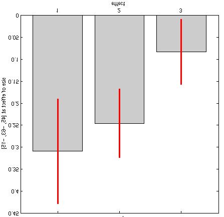
56 A C Figure 15 B D

57 A C Figure 16 B D

58 A C Figure D B