First Technical Course, European Centre for Soft Computing, Mieres, Spain. 4th July 2011

Transcription

1 First Technical Course, European Centre for Soft Computing, Mieres, Spain. 4th July 2011 Linear

2 Given probabilities p(a), p(b), and the joint probability p(a, B), we can write the conditional probabilities p(b A) = p(a B) = p(a, B) p(a) p(a, B) p(b) Linear Eliminating p(a, B) gives p(b A) = p(a B)p(B) p(a)

3 In the context of model fitting, if we have data y and model parameters w, the terms in p(w y) = p(y w)p(w) p(y) are referred to as the prior, p(w), the likelihood, p(y w), and the posterior, p(w y). The probability p(y) is a normalisation term and can be found by marginalisation. For continuously valued parameters p(y) = p(y w)p(w)dw or for discrete parameters p(y) = i p(y w i )p(w i ) p(y) is referred to as the marginal likelihood or model evidence. Linear

4 Johnson et al (2001) consider Bayesian inference in for Magnetic Resonance Angiography (MRA). An Aneurysm is a localized, blood-filled balloon-like bulge in the wall of a blood vessel. They commonly occur in arteries at the base of the brain. There are two tests: (1) MRA can miss sizable Intracranial Aneurysms (IA) s but is non-invasive (top). (2) Intra-Arterial Digital Subtraction Angiography (DSA) (bottom) is the gold standard method for detecting IA but is an invasive procedure requiring local injection of a contrast agent via a tube inserted into the relevant artery. Linear

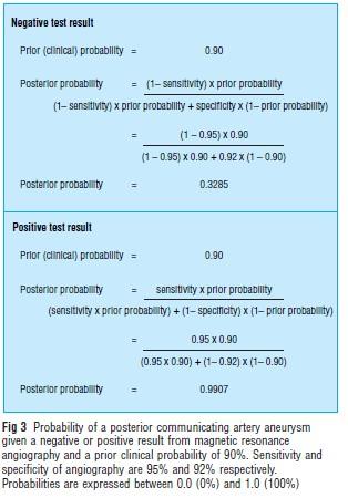
5 Given patient 1 s symptoms (oculomotor palsy), the prior probability of IA (prior to MRA) is believed to be 90%. For IAs bigger than 6mm MRA has a sensitivity and specificity of 95% and 92%. What then is the probability of IA given a negative MRA test result? Linear

6 The probability of IA given a negative test can be found from p(mra = 0 IA = 1)p(IA = 1) p(ia = 1 MRA = 0) = p(mra = 0 IA = 1)p(IA = 1) + p(mra = 0 IA = 0)p(IA = 0) where p(ia = 1) is the probability of IA prior to the MRA test. MRA test sensitivity and specificity are p(mra = 1 IA = 1) p(mra = 0 IA = 0) We have p(mra = 0 IA = 1) = 1 p(mra = 1 IA = 1) Linear

7 Linear

8 Linear A negative MRA cannot therefore be used to exclude a diagnosis of IA. In both reported cases IA was initially excluded, until other symptoms developed or other tests also proved negative.

9 For the prior (blue) we have m 0 = 20, λ 0 = 1 and for the likelihood (red) m D = 25 and λ D = 3. Linear Precision, λ, is inverse variance.

10 for Gaussians For a Gaussian prior with mean m 0 and precision λ 0, and a Gaussian likelihood with mean m D and precision λ D the posterior is Gaussian with λ = λ 0 + λ D m = λ 0 λ m 0 + λ D λ m D So, (1) precisions add and (2) the posterior mean is the sum of the prior and data means, but each weighted by their relative precision. Linear

11 for Gaussians For the prior (blue) m 0 = 20, λ 0 = 1 and the likelihood (red) m D = 25 and λ D = 3, the posterior (magenta) shows the posterior distribution with m = and λ = 4. Linear The posterior is closer to the likelihood because the likelihood has higher precision.

12 General Linear Model The General Linear Model (GLM) is given by y = Xw + e where y are data, X is a design matrix, and e are zero mean Gaussian errors with covariance V. The above equation implicitly defines the likelihood function p(y w) = N(y; Xw, C y ) where the Normal density is given by ( 1 N(x; µ, C) = (2π) N/2 exp 1 ) C 1/2 2 (x µ)t C 1 (x µ) Linear

13 Maximum Likelihood If we know C y then we can estimate w by maximising the likelihood or equivalently the log-likelihood L = N 2 log 2π 1 2 log C y 1 2 (y Xw)T Cy 1 (y Xw) We can compute the gradient with help from the Matrix Reference Manual dl dw = X T Cy 1 y X T Cy 1 Xw to zero. This leads to the solution ŵ ML = (X T C 1 y X) 1 X T C 1 y This is the Maximum Likelihood (ML) solution. y Linear

14 fmri time series analysis In software such as SPM or FSL brain mapping is implemented with the following method. At the ith voxel (volume element) we have time series y i Linear

15 fmri time series analysis In a standard analysis linear models are fitted separately at each voxel y i = Xw i + e i C y = Cov(e i ) is the error covariance and then the regression coefficients are computed using Maximum Likelihood (ML) estimation ŵ i = (X T C 1 y X) 1 X T C 1 The fitted responses are then ŷ i = Xŵ i y y i Linear

16 Statistical Parametric Maps We can then test if effects are significantly non-zero. The uncertainty in the ML estimates is given by A t-score is then given by S = (X T Cy 1 X) 1 t i = ŵ i (k)/ S(k, k) Linear

17 The standard approach in SPM and FSL smooths the data, y, before fitting time series models at each voxel. This increases the SNR. Linear Top 3 views show original fmri images, bottom 3 views show data smoothed by a Gaussian kernel of width 6mm.

18 Generally, we are looking to test for multiple effects at each point in the brain. Linear Henson et al. (2002) was looking to find which brain regions show different responses for repeated and familiar stimuli in the context of face processing.

19 Generally, we are looking to test for multiple effects at each point in the brain. Linear

20 Generally, we are looking to test for multiple effects at each point in the brain. At voxel i y i = Xw i + e i where eg. X is as below and w i is a 4-element vector. Linear

21 Contrast vectors c can then be used to test for specific effects µ c = c T ŵ i For example, to look at the average response to faces (regardless of type) c = [1/4, 1/4, 1/4, 1/4]. The uncertainty in the effect is then σ 2 c = c T Sc and a t-score is then given by t = µ c /σ c Linear

22 To look at the effect of repetition c = [1/2, 1/2, 1/2, 1/2]. Linear

23 Bayesian GLM A Bayesian GLM is defined as y = Xw + e 1 w = µ w + e 2 where the errors are zero mean Gaussian with covariances Cov[e 1 ] = C y and Cov[e 2 ] = C w. p(y w) = N(y; Xw, C y ) p(w) = N(w; µ w, C w ) Linear

24 GLM posterior The posterior density is (Bishop, 2006) p(w y) = N(w; m w, S w ) Sw 1 = X T Cy 1 X + Cw 1 m w = S w (X T Cy 1 y + Cw 1 µ w ) The posterior precision is the sum of the prior precision and the data precision. The posterior mean is a relative precision weighted combination of the data mean and the prior mean. Linear

25 Bayesian GLM with two parameters The prior has mean µ w = [0, 0] T (cross) and precision C 1 w = diag([1, 1]). Linear

26 Bayesian GLM with two parameters The likelihood has mean X T y = [3, 2] T (circle) and precision (X T C 1 y X) 1 = diag([10, 1]). Linear

27 Bayesian GLM with two parameters The posterior has mean m = [2.73, 1] T (cross) and precision S 1 w = diag([11, 2]). Linear

28 Bayesian GLM with two parameters In this example, the measurements are more informative about w 1 than w 2. This is reflected in the posterior distribution. Linear

29 Shrinkage Prior If µ w = 0 we have a shrinkage prior. Linear

30 Tennis From Wolpert and Ghahramani (2006) Linear p(w y) = N(m w, S w ) Sw 1 = X T Cy 1 X + Cw 1 m w = S w (X T Cy 1 y + Cw 1 µ w ) There is evidence that humans combine information in this optimal way (Doya et al 2006).

31 Time series models Usually, we wish to test for multiple experimental effects. At the ith spatial position y i = Xw i + e i where eg X is a T K design matrix as below and w i is a K = 4 element vector and y i is a T = 351 element time series Linear

32 Time series model for images We can write the model over all spatial positions i = 1..V as Y = XW + E where Y is an T V fmri data matrix, X is a V K design matrix, W is a K V matrix of regression coefficients, and E is an T V matrix of errors. The ith column of Y is the time series at the ith voxel. The ith column of W, w i, is the vector of regression coefficients at the ith voxel. Linear The kth row of W, w k, is a V -element vector. It contains the image of regression coefficients for the kth effect we are testing for.

33 We can define a spatial prior over each of the k = 1..K regression coefficient images p(w k α) = N(w k ; 0, αq w ) to capture our prior information that regression coefficients will be similar at nearby voxels, where the larger α produces smoother images. Linear The matrix Q w can be set to reflect different assumptions abouth the types of smoothness.

34 Laplacian Prior If we define a spatial kernel S with elements Linear Then z k = Sw k will be a vector of local discrepancies between neighbouring voxels. The quantity z T k z k = w T k ST Sw k is then the sum of squared discrepancies. A shrinkage prior on z k, that is one that encourages minimal discrepancy, is given by where Q 1 w = S T S. p(w k α k ) = N(w k ; 0, α k Q w )

35 We define a spatio-temporal model where p(y, W ) = p(y W )p(w α) p(w α) = K p(w k α k ) k=1 Linear Different effects (eg first versus second presentation) can have different smoothnesses. For full generative model see Penny et al (2005).

36 Variational Bayes Given fmri data, the posterior distibution for the spatio-temporal model is Gaussian but the posterior covariance is of dimension VK VK which is too large to handle. Instead we use an approximate posterior that factorises over voxels q(w Y ) = q(w i Y ) i This approximate posterior can be fitted using the Variational Bayes (VB) framework (Bishop 2006, Penny et al. 2005). The VB method can also be used to estimate the prior precisions α. This is a special case of (see MEG example later). Linear

37 Results. (a) Structural image (MRI) (b) ML applied to smooth data Y (c) Bayesian inference with Global shrinkage prior (Q w = I) (d) Bayesian inference with Laplacian prior (Q w = S T S) Linear For (c) a Gaussian smoothing kernel of 8mm FWHM was used.

38 . (a) True activations (b) ML applied to smooth data (c) Bayesian inference with Global shrinkage prior (Q w = I) (d) Bayesian inference with Laplacian prior (Q w = S T S) Linear

39 Receiver Operating Characteristic Linear

40 is achieved through inversion of the linear model y = Xw + e (d 1) = (d p)(p 1) + (d 1) for MEG data, y with d sensors and p potential sources, w, lying perpendicular to the cortical surface. The lead field matrix is specified by X. For our example we have d = 274 and p = Linear The above equation is for a single time point.

41 Generative Likelihood Prior We let p(y w) = N(y; Xw, C y ) p(w) = N(w; 0, C w ) Linear C y = λ y Q 1 C w = λ w Q 2 For shrinkage priors Q 2 = I p, MAP estimation results in the minimum norm method of source reconstruction. This is implemented in SPM as the IID option

42 Smoothness Priors For smoothness priors Q 2 = KK T corresponding to the operation of a Gaussian smoothing kernel, MAP estimation results something similar to the Low Resolution Tomography (LORETA) method. Linear This is implemented in SPM as the COH option. Note, these are not location priors.

43 Posterior Density From earlier we have where p(w y) = N(w; m w, S w ) S 1 w = X T Cy 1 X + Cw 1 m w = S w X T Cy 1 y However, S w is p p with p = 8192 so cannot be inverted easily. But we can use the matrix inversion lemma, also known as the Woodbury identity (Bishop, 2006) (A + BCD) 1 = A 1 A 1 B(C 1 + DA 1 B) 1 DA 1 to ensure that only d d matrices need inverting. Linear

44 Simulation Two sinusoidal sources were placed in bilateral auditory cortex and produced this MEG data (Barnes, 2010), comprising d = 274 time series (butterfly plot) Linear

45 LORETA We fix λ y = 1. Here we set λ w = Linear This shows the posterior mean activity for the 500 dipoles with the greatest power (over peristimulus time)

46 LORETA We fix λ y = 1. Here we set λ w = 0.1. Linear

47 LORETA We fix λ y = 1. Here we set λ w = 1. Linear

48 Hyperparameters, λ, can be estimated so as to maximise the model evidence. This forms the basis of Empirical Bayes. The marginal likelihood or model evidence is given by p(y λ) = p(y, w, λ)dw = p(y w, λ)p(w λ)dw The log model evidence is L(λ) = log p(y λ) For linear models this can be derived as in Bishop (2006) or as in my Maths for Brain Imaging notes. In this formulation λ are not treated as random variables. There is no prior on them. Linear

49 We iterate between finding the parameters w and hyperparameters λ. For linear Gaussian models this corresponds to computing the posterior over w S 1 w = X T Cy 1 X + Cw 1 m w = S w (X T Cy 1 y + Cw 1 µ w ) and then setting λ to maximise the model evidence. Linear ˆλ = arg max L(λ) λ These two steps are then iterated and can be thought of as E and M steps in an EM optimisation algorithm.

50 The model evidence is composed of sum squared precision weighted prediction errors and Occam factors L(λ) = 1 2 et y Cy 1 e y 1 2 log C y d log 2π et wcw 1 e w 1 2 log C w S w where λ is a vector of hyperparameters that parameterise the covariances C w = λ w Q w and C y = λ y Q y. The prediction errors are the difference between what is expected and what is observed e y = y Xm w e w = m w µ w Linear

51 For a Bayesian GLM y = Xw + e 1 w = µ w + e 2 with isotropic covariances (eg minimum norm source reconstruction) C y = λ y I N C w = λ w I p and d data points and p parameters. The equations for updating λ can be derived as shown in Chapter 10 of Bishop (2005). Linear

52 Well-determined parameters Define γ = p j=1 α j α j + ˆλ w where α j are eigenvalues of the data precision term X T Cy 1 X. If α j >> ˆλ w for all j then γ = p. Parameters have all been determined by the data. So γ is equivalent to number of well-determined parameters. Linear

53 M-Step Then 1 ˆλ w = et we w γ 1 ˆλ y = et y e y d γ Linear where the prediction errors are e y = y Xm w e w = m w µ w This effectively partitions the degrees of freedom in the data into those for estimating the prior and the likelihood. Setting λ to maximise the marginal likelihood produces unbiased estimates of variances whereas ML estimation produces biased estimates.

54 For a Bayesian GLM with covariances y = Xw + e 1 w = µ w + e 2 C y = i λ i Q i C w = i λ i Q i where Q are known covariance basis functions. The M-step is ˆλ = arg max L(λ) λ Linear

55 This maximisation is effected by first computing the gradient and curvature of L(λ) at the current parameter estimate, λ old j λ (i) = dl(λ) dλ(i) H λ (i, j) = d 2 L(λ) dλ(i)dλ(j) where i and j index the ith and jth parameters, j λ is the gradient vector and H λ is the curvature matrix. The new estimate is then given by λ new = λ old H 1 λ j λ Linear

56 Hyperparameters set using. Linear The minimum norm method, also implemented in SPM as the IID option.

57 Smoothness Priors Hyperparameters set using. Linear This is similar to the LORETA method, implemented in SPM as the COH option.

58 G. Barnes (2010) Localisation, SPM Manual, Chapter 35 C. Bishop (2006) Pattern Recognition and Machine Learning, Springer. K. Doya et al (2006) Bayesian Brain. Probabilistic approaches to neural coding. MIT Press. R. Henson (2003) Cerebral Cortex, 12: M. Johnson et al. (2001) BMJ 322, D. Mackay (2003) Information Theory, Inference and Learning Algorithms, Cambridge. W. Penny et al. (2007) time series analysis with spatial priors. Neuroimage 24, D. Wolpert and Z. Ghahramani (2004) In Gregory RL (ed) Oxford Companion to the Mind, OUP. Linear