Linear Models for Regression

Transcription

1 Linear Models for Regression Seungjin Choi Department of Computer Science and Engineering Pohang University of Science and Technology 77 Cheongam-ro, Nam-gu, Pohang 37673, Korea / 36

2 Outline Regression Least Squares Method Ridge Regression Least Mean Squares Recursive (Sequential) least squares Bias-Variance Dilemman Bayesian Linear Regression 2 / 36

3 Regression Regression aims at modeling the dependence of a response Y on a covariate X. In other words, the goal of regression is to predict the value of one or more continuous target variables y given the value of input vector x. The regression model is described by y = f (x) + ɛ. Terminology: x: input, independent variable, predictor, regressor, covariate y: output, dependent variable, response The dependence of a response on a covariate is captured via a conditional probability distribution, p(y x). Depending on f (x), Linear regression: f (x) = M j= w jφ j (x) + w. Kernel regression: f (x) = N i= w ik(x, x i ) + w. 3 / 36

4 Regression Function: Conditional Mean We consider the mean squared error and find the MMSE estiamte: E(f ) = y f (x) 2 = y f (x) 2 p(x, y)dxdy = y f (x) 2 p(x)p(y x)dxdy = p(x) y f (x) 2 p(y x)dy dx }{{} to be minimized [ f (x) y f (x) 2 p(y x)dy ] = f (x) = yp(y x)dy = y x. 4 / 36

5 Linear Regression Linear regression refers to a model in which the conditional mean of y given the value of x is an affine function of φ(x) f (x) = M w j φ j (x) + w φ (x) = w φ(x), j= where φ j (x) are known as basis functions and w = [w, w,..., w M ], φ = [φ, φ,..., φ M ]. By using nonlinear basis functions, we allow the function f (x) to be a nonlinear function of the input vector x (but a linear function of φ(x)). 5 / 36

6 Polynomial Regression: y t = M j= w jφ j (x t) = M j= w jx j t M = M = t t x x M = 3 M = 9 t t x x 6 / 36

7 Basis Functions Polynomial regression: φ j (x) = x j. Gaussian basis functions: φ j (x) = exp { x µ j 2 2σ 2 }. Spline basis functions: Piecewise polynomials (divide the input space up into regions and fit a different polynomial in each region). Many other possible basis functions: sigmoidal basis functions, hyperbolic tangent basis functions, Fourier basis, wavelet basis, and so on. 7 / 36

8 Least Squares Method Given a set of training data {(x t, y t )} N t=, we determine the weight vector w which minimizes E LS = 2 N t= { yt w φ(x t ) } 2 = 2 y Φw 2, where y = [y,..., y N ] and Φ R N (M+) is known as the design matrix with Φ tj = φ j (x t ), i.e., φ (x ) φ (x ) φ M (x ) φ (x 2 ) φ (x 2 ) φ M (x 2 ) Φ = φ (x N ) φ (x N ) φ M (x N ) 8 / 36

9 E LS w = leads to the normal equation that is of the form Φ Φw = Φ y. Thus, LS estimate of w is given by w LS = ( Φ Φ) Φ y = Φ y, where Φ is known as the Moore-Penrose pseudo-inverse. Φ Φ is known as the Gram matrix. 9 / 36

10 Maximum Likelihood We assume that the target variable y t is given by a deterministic function f (x t, w) = w φ(x t ) with additive Gaussian noise so that where ɛ N (, σ 2 I ). The log-likelihood is given by y = Φw + ɛ, L = log p(y Φ, w) = N log p(y t φ(x t ), w) t= = N 2 log σ2 N 2 log 2π σ 2 E LS. Therefore, under Gaussian noise assumption, w ML = w LS. / 36

11 Ridge Regression We consider the sum-of-squares error function with a Euclidean norm-based regularizer Solving E w E = y Φw 2 + λ } 2 {{} 2 w 2. }{{} LSfit regularizer = for w leads to w ridge = ( λi + Φ Φ) Φ y. / 36

12 Ridge Regression: MAP Perpective Recall the likelihood: p(y Φ, w) = N (y Φw, σ 2 I ). Assume a zero-mean Gaussian prior with covariance Σ for parameters w: Then the posterior over w, p(w y, Φ) = p(w) = N (w, Σ). p(y Φ, w)p(w), p(y Φ, w)p(w)dw is still Gaussian with mean and mode at ŵ = (σ 2 Σ + Φ Φ) Φ y. When Σ is proportional to identity, i.e., Σ = λ σ 2 I, this is called ridge regression. 2 / 36

13 Ridge Regression: Shrinkage Suppose that the SVD of the design matrix Φ R N (M+) has the form Φ = UDV, where D = diag(d,..., d M+ ). Using the SVD we write the least squares fitted vector as ( M+ Φw LS = Φ Φ Φ) Φ y = UU y = u i u i y, where U y are the coordinates of y with respect to the orthonormal basis U. The ridge solutions are ( Φw ridge = Φ λi + Φ Φ) Φ y i= M+ = UD(D 2 + λi ) DU di 2 y = u i di 2 + λ u i y. It shrinks the coordinates by the factors. A greater amount of d i 2 +λ shrinkage is applied to basis vectors with smaller di 2. d 2 i i= 3 / 36

14 Least Mean Square (LMS) LMS is a gradient-descent method which minimizes the instantaneous error E t, where E LS = N E t = 2 t= N t= { y t w φ(x t)} 2. The gradient descent method leads to the updating rule for w that is of the form w w η E t { } w + η y t w φ(x t) φ(x t), where η > is a constant known as learning rate. 4 / 36

15 Recursive (Sequential) LS We introduce the forgetting factor λ to de-emphasize old samples, leading to the following error function E RLS = 2 t λ t i (y i φ i w t ) 2, i= where φ t = φ(x t). Solving E RLS w t = for w t leads to [ t ] [ t ] λ t i φ i φ i w t = λ t i y i φ i. i= i= 5 / 36

16 We define P t = r t = [ t ] λ t i φ i φ i, i= [ t ] λ t i y i φ i. i= With these definitions, we have w t = P tr t. The core idea of RLS is to apply the matrix inversion lemma to develop the sequential algorithm without matrix inversion. (A + BCD) = A A B(DA B + C ) DA. 6 / 36

17 The recursion for P t is given by [ t P t = λ t i φ i φ i = = λ i= ] [ t λ λ t i φ i φ i i= + φ t φ t ] [ P t Pt φ ] t φ t Pt. (matrix inversion lemma) λ + φ t P t φ t 7 / 36

18 Thus, the updating rule for w is given by w t = P tr t = [ P t Pt φ ] tφ t P t λ λ + φ t Pt φ [λr t + y tφ t ] t ] [y t φ t w t P t φ t = w t + λ + φ t Pt φ t }{{} gain } {{ } error. 8 / 36

19 Expected Loss The squared loss L is given by L(y, f (x)) = (f (x) y) 2. The expected loss is computed by E {L(y, f (x))} = (f (x) y) 2 p(x, y)dxdy = E {(f (x) E{y x} + E{y x} y) 2} = E {(f (x) E{y x}) 2 + (E{y x} y) 2} + 2E {(f (x) E{y x}) (E{y x} y)}. }{{} 9 / 36

20 The expected loss can be written as E {L(y, f (x))} = (f (x) E{y x}) 2 p(x)dx } {{ } first term + (E{y x} y) 2 p(x)dx. } {{ } second term The function f (x) appears only in the first term which will be minimized when f (x) = E{y x}. The second term is the variance of the distribution of y, averaged over x, representing the intrinsic variability of the target data and can be regarded as noise. Because it is independent of f (x), it represents the irreducible minimum value of the loss function. 2 / 36

21 Bias-Variance Decomposition Consider the integrand of the first term, which for a particular data set D takes the form (f (x; D) E{y x}) 2. Then we have { E D (f (x; D) E{y x}) 2} = (E D{f (x; D)} E{y x}) 2 }{{} (bias) { 2 + E D (f (x; D) E D{f (x; D)}) 2}. } {{ } variance expected loss = (bias) 2 + variance + noise. 2 / 36

22 Bias-Variance Dilemma There is a trade-off between bias and variance: flexible models: low bias but high variance rigid models: high bias but low variance The model with the optimal predictive capability is the one that leads to the best balance between bias and variance. 22 / 36

23 Example We consider the sinusoidal data set. We generate data sets, each containing N = 25 data points, independently from the sinusoidal curve h(x) = E{y x} = sin(2πx). The data sets are indexed by l =,..., L where L =. For each data set D (l), we fit a model with 24 Gaussian basis functions through a method of ridge regression to give a prediction function f (l) (x). f (x) = L (bias) 2 = N variance = N L f (l) (x), l= N [ f (xt) h(x ] 2 t), t= N t= L L l= [ f (l) (x t) f (x t)] / 36

24 Rigid model (st row) and flexible model (2nd row) low variance high bias high variance low bias 24 / 36

25 Bayesian Linear Regression The likelihood function is given by p(y Φ, w) = N p(y t φ t, w), t= where p(y t φ t, w) = N (y t w φ t, β ). Assuming Gaussian prior for w, i.e., p(w) = N (w µ, Σ ), the posterior distribution over w is again Gaussian that is of the form where p(w y, Φ) = N (w µ N, Σ N ), µ N = Σ N (Σ µ + βφ y), Σ N = Σ + βφ Φ. 25 / 36

26 For the sake of simplicity, we consider a particular form of Gaussian prior (zero mean isotropic Gaussian prior), p(w α) = N (w, α I ). Then the corresponding posterior distribution over w is given by where p(w y) = N (w µ N, Σ N ), µ N = βσ N Φ y, Σ N = αi + βφ Φ. 26 / 36

27 An Example of Sequential Bayesian Learning Consider a linear model y = w + w x where only two parameters are involved. Next slide illustrates the sequential nature of Bayesian learning, showing that the posterior distribution over parameters become sharper as more data points are observed. Left-hand column: likelihood, p(y x, w). Middle column: prior/posterior, p(w D t). Right-hand column: samples of function y = w + w x where w are drawn from the posterior. 27 / 36

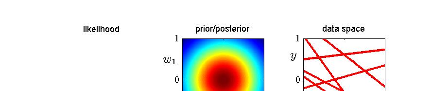
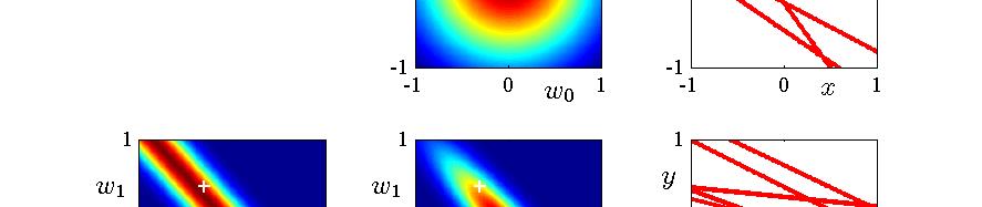
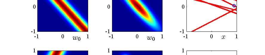
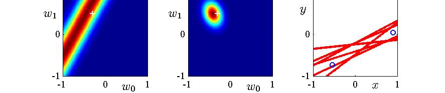
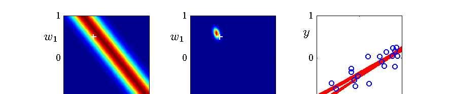
28 28 / 36

29 Predictive Distribution Make predictions of y for new values x (i.e, φ ). Let D = {Φ, y}. Then the predictive distribution is given by p(y φ, D, α, β) = p(y φ, w, β)p(w D, α, β)dw ( ) = N y µ N φ, σ2 N(x ), where µ N = βσ N Φ y, Σ N = αi + βφ Φ, σn(x 2 ) = + φ β Σ Nφ. }{{}}{{} uncertainty associated with parameters w noise on the data 29 / 36

30 Examples of Predictive Distributions t t x x t t x x 3 / 36

31 Plots of f (x; w) using samples from p(w y) t t x x t t x x 3 / 36

32 Bayesian Model Comparison Avoid the over-fitting associated with maximum likelihood by marginalizing over the model parameters instead of making point estimates of their values. Models can be compared directly on the training data, without the need for a validation set. Avoids the multiple training runs for each model associated with cross-validation. 32 / 36

33 Suppose that we wish to compare a set of L models, {M i } for i =,..., L. (a model refers to a probability distribution over the observed data D) Given a training set D, we then wish to evaluate the posterior distribution p(m i D) p(m i ) p(d M i ). }{{}}{{} prior evidence p(m i ) is a prior probability distribution to express our uncertainty. The data is generated from one of these models but we are uncertain which one. p(d M i ) is the model evidence which expresses the preference shown by the data for different models. This is also known as marginal likelihood, since it can be viewed as a likelihood function over the space of models, in which the parameters have been marginalized out. 33 / 36

34 Bayes factor is the ratio of model evidences for two models: p(d M i ) p(d M j ). Model selection: Choose the single most probable model. For a model governed by a set of parameters w, the model evidence is given by p(d M i ) = p(d w, M i )p(w M i )dw. 34 / 36

35 p(d) M M 2 M 3 D D M is the simplest and M 3 is the most complex. For the particular observed data set D, the model M 2 with intermediate complexity has the largest evidence. 35 / 36

36 Marginal Likelihood: Hyperparameter Estimation We estimate hyperparameters α and β through maximizing the marginal likelihood. The marginal likelihood is given by p(y Φ, α, β) = p(y Φ, w, β)p(w α)dw. Marginal likelihood maximization is illustrated in detail in Sec and / 36