Towards the thermodynamic characterization of an hybrid Pulsating Heat Pipe in micro-gravity conditions through parabolic flight campaigns

Transcription

1 UNIVERSITA DEGLI STUDI DI PADOVA Dipartimento di Ingegneria Industriale DII Corso di Laurea Magistrale in Ingegneria Aerospaziale Towards the thermodynamic characterization of an hybrid Pulsating Heat Pipe in micro-gravity conditions through parabolic flight campaigns Relatore: Prof.ssa Luisa Rossetto Co-Relatore: Prof. Marco Marengo Marco Bernagozzi matr: Anno Accademico 2015/2016

2 Abstract In the past years, growing demand of high thermal performances in front of low costs has pushed the development of brilliant two-phase based devices. Among the most promising there is the Pulsating Heat Pipes (PHP), which is a bended evacuated tube partially filled with a working fluid that oscillates thanks to thermally driven pressure differences. PHP opens new possibilities in terms of performances, simplicity, maintenance, cost and gravity independence. The working principle depends strictly on the internal diameter of the pipe, that if it is chosen smaller than the critical diameter for that specific fluid, allows a slug and plug regime, characterized by an alternation of liquid slug and vapor bubbles, responsible of the heat transfer. In space applications, critical diameter threshold rises because gravity decreases, allowing to employ bigger cross sections for the pipe, thus leading to bigger capabilities of heat removal. In order to exploit this, a new concept of PHP that on Earth works like a thermosyphons while in space it works like a PHP was created: the Hybrid Pulsating Heat Pipe. The preferred solution to test this device in microgravity is the Parabolic Flight and in order to be accepted on this platform, an interface between the actual experiment and the aircraft needs to be designed. Hence, the two objectives of this work: to create the primary structure of this interface, trying to make it compatible with new future applications and resistant to emergency landing loads; to verify the application of a novel lumped parameter model, used for a standard PHP, on the geometry of a Hybrid-PHP. For the numerical analysis, results showed that the code is not applicable to the chosen geometry, because the diameter is too big to allow a proper generation of bubbles. While for the primary structure, two models were created, one following the suggested solutions of the company ruling the flight, the other trying to keep overall mass to a minimum. A FEM analysis was performed on both models, showing satisfying results since yield stress was never reached. i

3 Abstract ii

4 Contents Abstract... i Introduction... 1 Chapter 1 - Pulsating Heat Pipes Introduction Two-Phase Flow Boiling Flow Patterns Taylor Bubble Flow Thermal efficiency parameters Pulsating Heat Pipes Working Principles Advantages Applications Thermosyphons Hybrid Heat Pipe Chapter 2 - PHP Numerical Modelling Introduction Previous Model Continuum wave propagation Spring-Mass-Damper approach Lumped Parameters Approach Artificial Neural Networks (ANN) D or 3D Volume Of Fluid (VOF) approach Novel Model Solid Model i

5 Contents Fluidic Model Coupling of Solid and Fluidic Model Model Validation Previous Validation New Validation Further Developments Chapter 3 - Parabolic Flights Introduction Useful Definitions Microgravity platforms comparisons Parabolic Manuever Chapter 4 - Primary Structure Introduction Structure Design Mechanical Assessment Preliminary Analysis Linear Load Light Configuration Chapter 5 - FEM Analysis Introduction Light Model Model Analysis Set Up Heavy Model Model ii

6 Introduction Analysis Set Up Results Light Model Heavy Model Results Summary Conclusions Appendix A - Simulations List Appendix B - Modes Shapes Index of Figures Index of Tables References Acknowledgments iii

7 Contents iv

8 Introduction The aim of this work is to design both a particular, innovative two-phase device and a structure supporting the thermo-fluid dynamic characterization of such device in microgravity conditions. The device, called Pulsating Heat Pipe, is a self-circulating flow system where heat is usually removed by condensation and the working fluid is circulating due to vapour expansion in a evaporator [1]. The best features of two-phase devices for thermal control are that they may be passive, it means they do not require electrical power to function, and that they offer advantages in terms of operation against gravity and maximum heat transport capability. In all their various applications they permit very flexible configurations, as a matter of fact they are used for heating, cooling, air conditioning and heat recovery, to name a few. Moreover they are suitable to cool electronic components and for thermal control in space applications [1]. An example of such thermal technology are Heat Pipes, high thermal conductance devices constituted by a sealed tube where the two-phase fluid evaporates in correspondence of the heating component and condense in correspondence of the radiator. There exist different versions of heat pipes: standard heat pipes, where the return of the condensate occurs through an appropriate internal wick; Loop Heat Pipes, which consists of a capillary pump (evaporator), a compensation chamber (reservoir) both of them containing a wick, then a condenser, and vapour and liquid transport lines made in smooth tubing [2]; Sorption Heat Pipes (SHP) that consists of an absorbent system at one end and at the other end they can have either a condenser or an evaporator depending on the use [3]; Pulsating Heat Pipe, small meandering, completely wickless tube, filled with both liquid slugs and vapour bubbles due to the small diameter of the tubes that allows the capillary action. In this last case, once the device gets in contact with a heat source, evaporation occurs and the fluid starts oscillating randomly allowing the heat to be transported to the colder zone [4]. The key point of these devices for space application is actually the capillary diameter that is little enough to allow surface tension to dominate over gravity forces, avoiding fluid stratification in the tube. The circulation of the liquid-vapour fluid is due to the sensible heat and cooling and phase-changes, not to the gravity action. When the gravity is playing a role, heat pipe devices are better called thermosyphon [5]. 1

9 Introduction The thermal device going to be designed and tested is a kind of hybrid Pulsating Heat Pipe, a device with a diameter working on ground as a thermosyphon (no capillary action) while in microgravity condition it works like a closed loop capillary PHP. This is possible because on ground level buoyancy is stronger than surface tension, while in microgravity conditions ii becomes weaker, i.e the capillary action is stronger and the liquid slugs are filling completely the tube section. So in space, this novel PHP technology can be effective, leading to a larger pipe diameter and therefore to a bigger amount of dissipated power. Since on ground operations, the hybrid PHP still presents a gravity influence, in order to measure its thermal performance in the capillary regime, microgravity experiments are mandatory. The present work was carried out at the University of Brighton, inside a project which aims to be accepted for the 66 th Parabolic Flight Campaign of the European Space Agency. Parabolic flights are a tool to perform microgravity experiments, providing, with respect to other microgravity platforms, high flexibility, important experiment dimensions, and the unbeatable aspect of presence of scientists on the aircraft during their experiments. A first introductive theoretical part on the PHP behaviour, focusing on the physical phenomena involved in this device is given, followed by numerical simulations using a previously developed 1-D lumped parameter code, and finally the mechanical design of the new rack of the University of Brighton is closing the thesis. The experimental test-rigs for the parabolic flights must be designed following the strict rules given by NOVESPACE, the company responsible for the managing and the safety of the flights. Such requirements go from dimension compliance to mechanical assessment and risk analysis. The peculiarity of the new rack will be its modularity. This term has two meanings: the first is that all the components and subsystems must be easy to replace, and the second is that the rack can host thermal characterization of many types of two-phase devices. A black box methodology was adopted, i.e. designing the rack assuming to ignore what will be inserted inside. The reason of this modular choice is due to the desire by the team in Brighton of using the rack as much as many times possible, even with the shortest notice. 2

10 Chapter 1 - Pulsating Heat Pipes 1.1 Introduction Heat transfer devices are one of the most important branches of thermodynamics. They are very widespread and widely used in space heating, different kinds of refrigeration, air conditioning, power stations, to name a few. Needs of higher performances at low cost, have pushed in the past decades the development of passive devices, mainly based on the phase change of a working fluid, such as Heat Pipes. Removal of heat flux generated by electronic components is an example of this demand of thermal exchange improvement, since in the past years they have become more and more precise, small and compact. With miniaturization, heat rejection from unit surface area has increased a lot creating the needs for extremely efficient new cooling systems. Cooling devices work absorbing heat from the payload and transporting it to a cold source for being disposed of. Heat Pipes use pressure gradients resulting from phase change to carry the working fluid, instead of using expensive mechanical components like pump, valves and moving parts which are expensive components and they can fail. Therefore heat pipe technology is an appealing alternative providing performance maximization, improved reliability and premature failures prevention. In space applications, bigger platforms and bigger dreams of space explorations are leading to bigger requirements of heat removal or collection by large radiators. Heat Pipe technology can drastically reduce the number of moving parts and therefore increase devices weight, lifetime and simplicity, all parameters quite important in the aerospace industry. Following this evolution, novel two-phase wickless passive systems has been developed in the past few years. They are already been used in a variety of engineering fields like: thermal management (electronics cooling, polymeric heat exchangers), heat recovery (thermal solar panels, hybrid TPV panels), and cooling of engines and batteries in 3

11 Pulsating Heat Pipes automotive and aerospace applications. But all that glitters isn t gold, in fact even if complex two-phase devices such as sintered or wicked heat pipes are already widely implemented in space applications, they present some cost issues to be used in space. In early 90 s a new wickless passive two-phase device was created, the Pulsating Heat Pipe (PHP). It is a thermally driven, cheap, simple, noiseless and efficient device exploiting an oscillating regime produced by cyclic phase change of a working fluid. The main drawback of this new technology is the working regime that is maybe still a little bit too limited, depending on the still not perfect knowing of the behaviour of operational and constructive parameters [6]. That s why in the recent years, many attempts were carried on to understand and predict the inner behaviour of this device, since although is really technologically simple, the physic is extremely complicated and still not well understood. In this chapter a comprehensive overview of PHP will be presented, starting from the basic notions of two-phase flow and finishing with the novelty of the Hybrid Pulsating Heat Pipe. 1.2 Two-Phase Flow Boiling Boiling is the physical phenomenon where vaporisation affects the entire liquid mass, not only its free surface (in that case it is called evaporation). Boiling starts when the temperature of the solid surface that is heating the liquid is greater than the saturation temperature of the liquid [7]. There are three types of boiling with heat exchange mechanism characteristics that are still not entirely interpreted, as matter of fact there are no general empirical or theoretical correlations able to interpret the process. These three types are [8]: 1. Nucleate Boiling (ABC): the most observed one, it requires just a small amount of superheat 1. It is characterized from the creation of bubbles from some random point along the surface, named nucleation sites. Superficial roughness of the pipe becomes an important factor in order to control nucleation sites and so to control the whole nucleate process. Increasing superheating will also increase bubbles number and heat flux; 1 Superheating happens when a liquid is not boiling even if its temperature is higher than its boiling point. While subcooling happens when a liquid exist at a temperature below its normal saturation point. 4

12 Two-Phase Flow 2. Transition Boiling (CD): bubbles starts to coalesce and heat flux drastically decrease, when increasing superheating even more; 3. Film Boiling: on the heating surface a continuous cover of vapor film generates from which bubbles leave at precise time intervals. This process is very inefficient in terms of heat exchange; Figure 1 - Different kind of boiling (credit to American Chemical Society) In Figure 1 these kind of boiling are described in relation to the heat flux and the amount of superheat T. For low values of T, until A, the heat exchange mechanism is attributed to natural convection of superheated liquid evaporating from the free surface. From A, bubbles starts to generate, but they condensate before getting to the free surface. Then the heat flux rapidly grows since B with bubbles getting to the free surface. Here just a minimal part of heat is given from the heating surface to the forming bubbles, the most part is transferred to the superheated liquid thanks to the great agitation created by the creation and disappearance of bubbles. Corresponding to a precise value of T, a maximum heat flux C is reached. Controlling heating surface temperature, it is possible to determine the curve to D, which is the gradual transition from nucleate boiling to film boiling where heat flux decreases due to vapor layer presence. From D film boiling starts, heat flux is due to conduction and radiation to the point where the latter constitutes the principal heat exchange mechanism. Controlling heat flux instead, makes the fluid unable to dispose of heat flux smaller that imposed ones and thus it goes directly to E [7]. 5

13 Pulsating Heat Pipes Flow Patterns The term flow pattern usually indicates when a liquid-gas two phase mixture distributes itself in a constant recognizable structure [9]. One property that is better to recall because it is of great importance in flow pattern determination is surface tension. Molecules in a liquid are attracted by the other adjacent liquid molecules. In the presence of a free surface, there is no more equilibrium between forces, hence the fluid will experience an inwards force. Surface tension is defined as the surface energy per area unit and that energy is equal to the work needed to move the surface of a quantity dx balancing that force [10]. It is a quantity related to the latent heat of vaporisation, since this indicates the force of attraction between liquid molecules. In the case of horizontal and vertical orientation of the pipe, flow patterns can be different due to gravity effect that lead to a stratification of the phases in the first case [9]. Starting from the flow patterns in vertical tube: Bubbly flow: high number of bubbles of various shape and size, typically spherical with radius way smaller than the pipe radius; Slug flow: as it is going to be explained later, this is critical for understanding PHPs behaviour; it happens when void fraction is increased and bubbles became so close that start to coalesce, creating larger bubbles and occupying nearly all the pipe diameter (bubble radius pipe radius). Bubbles in this operating regime are called Taylor bubbles that are the subject of the next section; Churn flow: a chaotic situation with fluid oscillating up and down but with a net upward flow; this chaotic situation is the result of gravity and shear forces having the same magnitude but opposite directions. In small diameter tubes this regime doesn t appear and the flow goes directly from slug to annular; Annular flow: liquid makes a thin film on the pipe wall while in the center vapor flows up. This happens when shear forces at the liquid-vapor interface become higher than gravity forces thanks to the high velocity of the gas over the liquid film. Thus the interface suffers from some high frequency perturbation; 6

14 Two-Phase Flow Wispy annular flow: raising flow rate, it can happen that gas entrains some liquid droplets in the middle of the flow, to the point that they may form transient coherent structures; Mist Flow: at very high vapour mass velocities there is a situations inverse of the bubbly flow, where liquid is destroyed in droplets carried by the continuous gas flow; In the following picture it is possible to see the order in which it is possible to encounter these flow regimes, starting to the onset of nucleate boiling with the bubbly flow and finishing with the mist flow where vapour quality is equal to 1: Figure 2 - Flow regimes distributions in a vertical channel (credit to Wolverine Tube Inc.) While for a horizontal tube: Bubbly flow: this usually happens at high liquid mass flow rate and it is characterised by a large number of bubbles in the liquid concentrated in the upper half of the tube, thanks to buoyancy forces; 7

15 Pulsating Heat Pipes Stratified flow: when vapor mass flow rate is low, the gas takes position on the top on the liquid creating a complete separation of the phases; the interface is constant and uninterrupted; Stratified-wavy flow: starting from the previous type of flow and rising gas velocity, the interface is no more undisturbed and waves start to form and to move in the direction of flow. Although their amplitude depends on the velocities of both liquid and gas, waves never reach the top wall of the tube; after the passage of the wave, a thin film of liquid remains on the wall; Intermittent flow: gas velocity becomes big enough to make waves wash the top wall of the tube; it can be recognised a regime where bigger waves reach the top of the wall and smaller waves in between. This regime is important since is a combination of two very important regime for the PHPs, plug flow and slug flow: o Plug flow (or elongated bubbles flow): liquid plugs separated by elongated gas bubbles with a diameter smaller than the pipe diameter, thus the liquid is continuous along all the pipe; o Slug flow: rising gas velocities, elongated bubbles starts to occupy the entire tube diameter. In this situation the liquid plugs could be seen as large high amplitude waves; Annular flow: keep on increasing vapor mass flow rate, liquid takes an annular shape creating a film around the gas, similar to the case in vertical flow but with a negative thickness gradient going from the bottom to the top of the tube. At the interface between gas and liquid there are waves and there is the possibility that droplets may be dispersed in the gas flow; Mist flow: due to very high flow rates of vapor, the liquid loses its integrity and gets dismantled from the wall as small droplets straying in the continuous gas phase; 8

16 Two-Phase Flow Figure 3 - Flow patterns in horizontal (credit to Wolverine Tube Inc.) The manifestation of these regimes depends on several properties like flow rates of gas and liquid, fluid properties like density, viscosity and surface tension, operating conditions like pressure, temperature and gravity and the geometric characteristic of the pipe like shape, diameter and inclination [11] Taylor Bubble Flow Taylor bubble flow is another way to call the slug flow regime due to the instability that generates the Taylor bubble, discovered by the homonym scientist in 1950 [12]. It was deeply studied in the recent past thanks to great mass and heat transport properties, thanks to a well-defined interface area [13]. This phenomenon is frequently utilized in various chemical processes applications apart from heat exchange like distillation [14], nano-particle synthesis [15] and homogeneously/ heterogeneously catalysed gas-liquid reactions [16]. It is characterized by gas bubbles that fill almost completely the channel, separated by liquid slugs and surrounded by a thin liquid film creating a sort of continuity through the liquid phase [17]. The result is a flow pattern that is not periodic in space nor in time, essentially laminar and predominately viscous. The bubbles assume an elongated capsular shape like a bullet with a hemispherical nose and tail blunt end (although in the PHP there is a meniscus region on either end). This provides an equivalent diameter multiple times bigger than the actual channel diameter, 9

17 Pulsating Heat Pipes hence the interfacial area between liquid and bubbles is very large and this enhances the liquid and mass transfer. Liquid film thickness surrounding bubbles can vary from the order of millimetres to micrometres, depending on a series of parameters like dimensions, geometry and velocity of the flux, since bubbles velocity differs from liquid velocity [18]. Three different hydrodynamics regions divide the flow around a single bubble: the gas bubble surrounded by the liquid film, a very turbulent liquid wake near the bubble tail and the far laminar wake region [19]. The different forces at stake in this phenomenon are [20]: Pressure forces that drives from high to low pressure F p A p L Inertial forces that makes the system resist to an actual change of state of motion F i ρu2 L Viscous forces that makes velocity gradient diminish F v μu L 2 Gravity and buoyancy forces that drives flow in gravitational field F g mg F b g p Surface tension force that tent to minimize surface area F s μu L 2 Liquid slugs and vapor bubbles experience internal viscous dissipation as well as wall shear stresses. Surface and viscous forces are dominant in small lengths since they are inversely proportional to length square (L 2 ). One of the reasons why this type of flow pattern was extensively been studied is because it can really help heat, mass and momentum transfer with respect to other patterns or to single-phase flow, thanks to the turbulence induced in the wake region by the passage of a bubble. That generates toroidal vortexes so the following bubble accelerates and assumes a distorted shape. This event extends itself to the following bubble increasing in this way the overall heat transfer rate [21] [22]. While for the mass 10

18 Two-Phase Flow transfer, it was find out that is largely influenced by the length and velocity of the liquid slugs [21]. A very significant parameter in event involving bubbles in contact with a solid surface is wettability. When a liquid comes in contact with a solid surface, its molecules undergo another source of attraction, different from that between them. Depending on if this force of attraction is positive or negative (i.e. attractive or repulsive) the fluid surface will curve upwards or downwards. Thus is not only a matter of fluid thermophysical properties but also of physical-chemical properties of the solid. A way to define wettability is using the contact angle ϑ, which can be defined theoretically by Young s equations [20]: σ sv σ sl σ lv cosθ = 0 ( 1.1) where in that formula are present respectively surface tension between surface and vapor (sv), surface and liquid (sl), liquid and vapor (lv). These three quantities are extremely hard to evaluate in real life condition since their theories are quite weak. Moreover equation ( 1.1) is valid only for plane and ideal surfaces in equilibrium conditions. It is general practice to measure θ macroscopically, using a length scale bigger than the one of intermolecular forces, in this way is possible to define three conditions [18]: Lyophilic: 0 < θ < 90 Lyophobic: 90 < θ < 150 Super-lyophobic: 150 < θ < 180 When a liquid is perfectly wetting, that means that the contact angle is 0 and the force between liquid and solid acts on the normal direction of the surface. Wetting is another important factor in PHP behaviour is because, for instance, on a wet surface the liquid distributes itself better, giving finer heat exchange possibilities in case of evaporation. Usually, operating PHPs are under pre-wetted conditions. Moreover this factor affects friction. The most interesting parameters of Taylor bubbles flow are: film thickness, bubbles shapes and velocities, lengths of bubbles and slugs, pressure drop. The latter is composed by the Figure 4 - Wetting characterization with contact angle (credit to S. Khandekar) 11

19 Pulsating Heat Pipes pressure drop in the liquid plug, the pressure drop around the end of the bubble and the pressure drop along the body of the bubble, which is null if gravity forces approach zero and if the shear in the gas phase is neglected. Zero gravity brings gas viscosity and density to be much smaller than liquid viscosity and density, so the gas in the bubble has constant pressure and a constant curvature if the liquid film thickness is constant as well. Thus that pressure drop cannot exist in the bubble body [23]. All these observations result in the typical jawtooth trend of the pressure inside the PHP pipe, which the next paragraph will explain. But the pressure drop is not something to take for granted, since there can be some differences in the contact angle between the top (advancing angle ϑ a ) and tail (receding angle ϑ r ) of the bubble, creating the so called contact angle hysteresis, as we can see in Figure 5. 2σ P cap = R ( cosθ a + cosθ r ) Figure 5- Contact angle hysteresis (Khandekar et al. 2002) This creates an additional pressure resistance that, if the number of plugs in the channel is high enough, will accumulate and damp PHP oscillating motion [17] Thermal efficiency parameters One way to evaluate heat transfer capability is the effective thermal resistance [24], which is defined as the difference between the temperature of the evaporator T e and the temperature of the condenser T c, all divided by the heat transferred by the device q, which is the heat flux input: R eff = T e T c q ( 1.2) It is possible to see that raising q, the overall thermal resistance decrease improving performances (but there is a limit on this argument that will be treated later). But in the end, this is the parameter to evaluate experimentally. Using the electrical analogy of heat transfer, this is the sum of the resistance of every component of the device, like the wall, the vapor phase and the liquid: 12

20 Two-Phase Flow R eff = (R w,i + R l,i + R v,i ) i ( 1.3) With R w = D ln ( ) D 2t w 2πk s L R l = h c S R v = ( T) v q Figure 6 - Heat exchange scheme in the slug plug regime Thermal resistance of the pipe wall Thermal resistance of the liquid Equivalent thermal resistance of the vapor flow ( 1.4) ( 1.5) ( 1.6) where k s and t w are respectively the thermal conductivity of the wall and its thickness, h c is the convection coefficient of the liquid, S the surface of the liquid involved in the heat exchange phenomenon and ( T) v is the saturation temperature variation caused by the variation of the vapor pressure difference between evaporator and condenser. On the other hand, to consider also surface and length of the apparatus, it is possible to use the effective thermal conductivity [24]: k eff = ql eff A c (T e T c ) ( 1.7) where A c is the total cross sectional area of the heat pipe device and L eff is the effective length, a parameter that depends on the heating and cooling configuration: if the heating or the cooling are applied to the very tips of the pipe where evaporator and condenser are placed, L eff is the same length of the tube; if the heat is added to the outer surface of the evaporator and it is removed from the outer surface of the condenser, which is the most common adopted solution, L eff is the distance between the two points in condenser and evaporator where the average temperatures are established. Effective thermal resistance and conductivity are linked by the following formula: 13

21 Pulsating Heat Pipes k eff = L eff A c R eff ( 1.8) 1.3 Pulsating Heat Pipes Working Principles Pulsating Heat Pipes technology was invented and patented by Akachi in 1990 [25] and later developed in two different forms [26]: Closed Loop: tube ends are connected to each other in an endless loop; Open Loop: tube ends are not connected to each other; essentially one long tube bent in multiple turns with both its ends sealed after being filled with the working fluid; In this work only the Closed Loop ones will be investigated, since it has be proven that they provide better heat transfer performances [27]. Closed Loop Pulsating Heat Pipes are a meandering capillary tube closed end to end forming a certain number of parallel channels, evacuated and partially filled with a working fluid that creates the slug plug flow pattern [1]. From the imagine below it can be seen that three parts divide the PHP: evaporator, which is a surface in contact with the high temperature source, adiabatic section where the heat is just transported and the condenser, which is a surface in contact with the low temperature heat sink. Usually evaporator and condenser are placed at the turns of the pipe. 14

22 Pulsating Heat Pipes Figure 7 - PHP scheme (credits to Khandekar 2010) Since the working principle arise from the capillary condition, inner tube diameter becomes crucial. Generally it is accepted that this condition happens when Bond number is equal to 2 [28], while other scientist proposed is Bo = 1,84 [29] but this value is less conservative. Bond number is the ratio between gravitational forces and surface tension: Bo = d g(ρ l ρ v ) σ And from that it is possible to calculate the maximum inner diameter: = 2 ( 1.9) σ d crit 2 g(ρ l ρ v ) ( 1.10) where σ is the surface tension, g is gravity and ρ l and ρ v are respectively liquid and vapor densities. This surface tension dominates over gravity forces and there is no phase stratification between liquid and vapor but an alternation of vapor bubbles and liquid slugs. PHP works when liquid and vapor both oscillate and circulate driven by pressure disequilibrium and phase change phenomena (film evaporation, flow boiling, film condensation): when heat power is provided to the evaporator section, the thin liquid film, which surrounds each vapor plug, evaporates and so bubbles expand reaching 15

23 Pulsating Heat Pipes higher pressures and temperatures; the fluid adjacent is pushed towards the condenser zone by the bubbles, where heat is absorbed by a cold source and condensation occurs within the vapor plugs nearby the wall surface; the contraction of the vapor bubbles after condensation adds more motive force to the fluid [30] creating a steady oscillatory regime. Furthermore, the total volume is fixed so the collapse of a vapor plug must be completely and simultaneals compensate by new liquid slug generation or expansion. [31]. That is why also this device is called an Oscillating Heat Pipe (OHP). This oscillation is responsible for the heat transport inside the PHP from evaporator to condenser. The following is a really nice image of an example of slug flow inside a single turn tube [32]: Figure 8 - Slug flow in a bended channel (Khandekar et al. 2003) But where does this oscillating flow generates from? The answer hides behind pressure distribution. If the interface between liquid and vapor phase is composed by two menisci of different radii, perpendicular to each other, a pressure gradient will generates, defined by the Laplace-Young equation: p = σ ( ) ( 1.11) r 1 r 2 This pressure gradient creates a pressure distribution similar to a jawtooth that is the driving force of the oscillatory motion [24]. 16

24 Pulsating Heat Pipes Figure 9 - Pressure distribution (credit to H. Ma) where P c is the pressure drop at the interface, P f,l and P f,v are pressure drops inside a liquid slug and vapor plug respectively. If this pressure distribution fails, due maybe to excessive pressure drops given by friction losses, oscillating motion can stop so more external heat as pumping power will be necessary. Vapor bubbles during condensation and evaporation are compressing and enlarging respectively, thus acting as springs in the system. Hence from a mechanical point of view, a PHP system is a typical mechanical multi DOF vibratory system, with masses (liquid slug) connected between each other by springs (vapor bubbles). Heat transfer results from a combination of sensible heat (convection) carried by the liquid slugs and latent heat (phase change) handed over by the vapor plugs. But, if the working regime is slug plug, latent heat has not much effect because evaporation and condensation phenomena are important just to maintain the oscillating flow. The mechanism of heat transfer is governed by sensible heat, in fact 90% of the total heat is exchanged this way [33]. Many experiments in the recent years involved PHPs, trying to create both experimental and theoretical model finalized to a deep understanding of their physics. The first meant to actually visualize the flow patterns and evaluate heat transfer capability, the latter meant to model analytically and numerically the behaviour of the PHP, in particular the role of capillary forces on the working process. 17

25 Pulsating Heat Pipes Flow motion is more evident in the vertical BHM case (BHM stands for Bottom Heated Mode, where the evaporator is in the lower section of the meandering pipe) with respect to the horizontal case [34]. As matter of fact, micro-gravity experiments became fundamental to separate the effect of gravity, whether it results in buoyancy or inertia forces. In these many experiments, six fundamental parameters emerged in influencing the PHP functioning [35]: 1. internal diameter of the pipe, d in, it is the requisite to have capillary regime; besides, having a bigger diameter results in lower values of thermal resistance thanks to lower friction losses and so it requires lower heat input flux to maintain oscillatory motion [35]; 2. filling ratio, γ, that is the ratio between the volume of the liquid hold by the pipe and the internal volume of the pipe. If γ is too low there will not be enough liquid to sustain oscillatory flow and eventually the evaporator might dry out; on the other hand if it is too much, bubbles generation is not adequate to pump oscillatory flow; that said, it has been proven that it exists an optimal filling ratio for each PHP which usually ranges between 0.35 and 0.65 [6]; 3. power source at the evaporator, Q ex, because in case the heat flux is definitely too high, the liquid slug can move between evaporator and condenser with such a high inertia that can pass through the cooling section undisturbed and goes directly to the heating section. In this way the flow pattern changes from oscillatory to circulating, and there are some studies saying that this is a better condition for heat exchange [36] [37]; but if the heat source keeps on increasing the flow will become annular, so that is another limitation; on the other hand, there is a minimum heat flux to activate oscillatory motion inside the PHP, called start up heat flux [38]; 4. number of turns, n, that influences the thermal performances and gravity independence of the PHP; raising the number of turns gives more distinguished points where heat can be added to the pipe; moreover in the bend it can be either a vapor plug or a liquid slug so heating can provide different results that lead to more pressure differences, thus helping the oscillatory motion. In fact with a proper number of turns a PHP can operate in every orientation, becoming really interesting for space applications [39] 18

26 Pulsating Heat Pipes 5. orientation, θ, influences not only two-phase flux thermal hydraulics but also thermal performances; as a matter of fact Bottom Heated Mode (BHM) is always a better configuration than horizontal, respectively with the gravity vector parallel (θ = 90 ) and normal (θ = 0 ) to the direction identified by the channels [40]; in the first case the flow is more stable and efficient while in the second case it is characterized by lower oscillation frequency; furthermore, vertical configuration is also sensible to gravity, in fact the thermal resistance in gravity assisted mode is lower and it performs more than two times better than the horizontal orientation; also gravity helps in BHM while in Top Heated Mode (THM) is not giving particular benefits in ground operation, while in microgravity operation, THM configuration works better than on ground [41]; in the end it is possible to say that, for a perfect 2D geometry, there is an analogy between tilting from vertical/horizontal on ground operations and passing from normal to microgravity conditions [42]; 6. working fluid When it comes to choose the working fluid there are a few parameters that are quite significant: viscosity, because reduces the pressure drop in the channel; surface tension because it determines the channel diameter affecting also the maximum dissipated heat; specific heat because it can increase the amount of heat that a single liquid slug can carries and it is responsible of the most part of transferred heat; thermal conductivity of the liquid, because it helps heat transfer speed in evaporation, condensation and forced convection and also can reduce temperature differences between evaporator and condenser; latent heat, because it helps to generate bubbles or to reduce start up time, to have more heat involved in the phase change process and it also affects evaporation rate of the fluid; density, because it can affect weight and gravity effect; pressure derivative over temperature, δp, because it helps to increase pressure variation inside the PHP and δt help start up process. But obviously, some of these parameters are bucking. For instance a working fluid with greater surface tension has larger capillary resistance but also has a bigger capillary diameter, thus a bigger mass flow rate, thus a bigger thermal conductivity. In fact, the actual influence of the surface tension on the PHP is a trade-off between these two viewpoints. On the other hand, since latent heat becomes predominant in thermal exchange phenomena, with a low heat input flux, a working fluid with low values of latent heat is preferable and vice versa with high heat input 19

27 Pulsating Heat Pipes flux. Some examples of working fluid are the two refrigerants R113 (Trichlorotrifluoroethane) and FC-72 (Perfluorohexane), where the first is better for small dimension and low level of heat flux input while the second is better for high heat flux input [43]. Another crucial factor is pipe material, which has to be compatible with the chosen working fluid, in order to not generate gas that can affect the filling ratio, so the PHP operation. Corrosion and outgassing, which is the release of gas from a metal after a certain amount of time, is also a phenomenon to consider and to avoid. Usually the chosen materials are copper and aluminium thanks of their high thermal conductivity and chemical compatibility with the most commonly used fluid. Tube section is important not only with regards its diameter but also regarding its shape. As a matter of fact if the section is not circular, capillary sub channels will arise from sharp edges and disturb the slug plug flow, altering it to stratified flow or annular, worsening the heat transfer capability [44]. Thus, all these operational parameters are directly linked together and this is one of the reasons why it is so difficult to model the behaviour of the PHP. As said, PHP is a serpentine bent tube forming a pattern between evaporator and condenser, but despite its construction simplicity this design can be hard to match with the geometry of the two radiators and it needs a material in order to make contact with them. Normally this is a flat metal plate with on top of that some machined grooves that replicate the tube shape and where the tube is going to be placed. This increases costs, weight and overall thermal resistance of the device. Alternatively it can be possible to choose a flat plate configuration, where the working fluid circulates into channels made in the plate, obtaining a more compact design. 20

28 Pulsating Heat Pipes Figure 10 - (a) tubular PHP and (b) flat plate PHP (credit to Ma 2015) But not only the configuration of evaporator and condenser, also their dimensions require attention since it is a parameter that influences the overall heat transfer. For instance, if the condenser is not big enough it will not dissipate enough heat, limiting maximum heat flux. About the maximum heat flux, for a closed loop pulsating heat pipe with a filling ratio of 50%, Khandekhar et al. [32] were able to estimate the maximum achievable heat flux with an accuracy of ±30 %: q = q 2πd in nl e = 0.54[exp(θ)] 0.48 Ka 0.47 Pr l 0.27 Ja 1.43 n 0.27 ( 1.12) where q is the heat transfer rate, d in is the inner diameter of the pipe, n is the number of turns, L e is the length of the evaporator section, ϑ is the inclination angle measured from horizontal, Pr l, Ka and Ja are respectively the liquid Prandtl, the Karman and the Jacob numbers [28]: Pr l = μc p k Ka = ρ l(p sat,e p sat,c )D 2 μ l 2 L eff Ja = c p,l(t sat,e T sat,c ) h lv Groll and Khandekhar in 2003 [31] were able to explain the thermodynamics analysis of a PHP with known temperatures of evaporator and condenser, by means of a pressure/enthalpy diagram: 21

29 Pulsating Heat Pipes Starting from point A, which is the evaporator inlet, it is possible to proceed with an explanation of the involved thermodynamic transformations: AB: constant pressure heat input combined with and isentropic rise of pressure due to vapor bubbles expansion; BD: adiabatic section between evaporator and condenser that brings to a reduction of adiabatic pressure; DE: passage between inlet and outlet of the condenser that brings to a constant pressure condensation but with negative isentropic work; EA: isenthalpic pressure drop in the consecutive adiabatic section that closes the cycle. This scheme, albeit clarifier, still contains a lot of assumptions thus is not enough to explain PHP behaviour yet. Regarding flow pattern inside an operating PHP, it was found out that there is a direct correlation with the heat input flux. Four different flow regimes were observed: low and high amplitude oscillation, oscillation with circulation and flow reversals (also called local flow direction switch), stable circulation [45]. Each of these regimes is characterized by a level of heat flux input and a peculiar frequency spectrum Advantages PHP technology has most of the advantages of the conventional Heat Pipes but in addition to that PHPs have some unique beneficial features [24]: temperature range extends from -195 C to the maximum temperature that the chosen working fluid allows; it can be created essentially in any shape; part of evaporator heat can be converted in kinetic energy of the working fluid; both liquid and vapor flow running in 22

30 Pulsating Heat Pipes the same direction so there is no interference because once the motion is established, the direction is arbitrary but it remains the same for the entire duration of the experience; thin liquid film presence helps to increase extremely evaporating and condensing heat transfer; oscillatory motion helps forced convection also; increasing evaporator power means increasing heat transport capabilities; wickless structure; it can be designed in a way that gravity has no effect. All these unique features contribute together to give these advantages: High Heat Transport: when heat is provided to the evaporator, some of that goes to the liquid slug while the rest goes to the vapor bubbles, since the thermal resistance of the film is very small due to its small thickness, an extra-high heat transfer coefficient is achieved; moreover, gradually increasing velocity the oscillating flow produces vortexes that further increase heat transfer coefficient; since the liquid slugs and vapor plugs are limited in length, they do not develop into a full flow, leading to another boost of heat transport capabilities. These three effects cause the PHP to have an ultra-high thermal conductivity, which was evaluated to be times greater than a copper rod of the same dimension [46]; High flexibility: it can be created in nearly every geometry because the tube can be bended in any shape, so it has a huge number of different configurations and applications; Cost: being cheap is one of the most interesting advantages, technologically speaking it is just a bended metal pipe with a really small diameter and so the cost is really near to that of the raw material; moreover, since it has no wick, pumps, valves or any moving part, it does not require maintenance; this also enhance its simplicity and fatigue life; Light: this last feature depends on the overall dimension, but with respect to the conventional heat pipes, the high ratio between fluid and gas helps to lessen the overall weight of the device. In conclusion, it is possible to make a comparison between performance of a wicked Heat Pipe and a Pulsating Heat Pipe: 23

31 Pulsating Heat Pipes Table 1 - Heat Pipes and PHP comparison Wicked HP PHP Temperature Range Water, C Water, C Radial heat flux 250 W/cm 2 30 W/cm 2 Axial heat flux 600 W/cm W/cm 2 Total power (geometry dependent) 200 W 3000 W Thermal Resistance 0.01 C/W 0.1 C/W Start-up time In the order of seconds A few minutes where with total power is the maximum power that the PHP can dispose of and start up time it the time needed to the oscillating regime to establish. So it is possible to see how low is the radial heat flux, due to the PHP small diameter, and the extremely high axial heat flux that allows a great efficiency of heat transfer Applications PHP are very promising technologies to provide high heat removal capabilities in local spot and uniform temperatures on computer chips. Flexible electronics are getting more and more interesting over the past few years due to their mechanical properties, lightweight and low prices. But they have a low heat conductibility that is limiting their applications, so they need some very precise and accurate cooling. To help this process, heat pipes of very small dimensions are needed, down to micro heat pipes. Since they are easier to manufacture in micro scale, PHP are gaining more and more attention [47]. In these regards, Miyazaki [48] created a flexible closed loop pulsating heat pipe for notebooks cooling, dissipating heat from the CPU to the back of the display. They can be useful for chips cooling [49] or LED cooling [50]. PHPs also were proposed to reduce dimensions of a solar water heater, which is a renewable energy sunlight conversion for water heating using a solar thermal collector. It was shown that PHPs provide with respect standard heat pipes a good cost alternative and a pretty good efficiency of 76% [51]. Or either they can be used to recover waste heat after a drying process [52]. 24

32 Thermosyphons Eventually the need could be also for air preheating and water pumping [43], thermal management in hybrid vehicle [53], to cool fuel cell stocks [54]. PHPs are TRL 3 while standard heat pipes are TRL 9. Technological Readiness Level (TRL) it s a scale that indicates a methodology for assessing the degree of maturity of technology, originally developed by NASA in 1974 [55]. This scale goes from 1 to 9 where 1 is basic principles observed and 9 is actual system proven in operational environment. TRL means experimental proof of concept. The reason of this position is that there are scarce means to reliably predict PHPs performance because its fluid motion is inherently non-stationary and chaotic. Last, a new branch of research regards the implementation of PHPs in cryocoolers systems [56], generating the so called cryogenic pulsating heat pipes. The idea is to use the PHP to spread cooling from the cold head region of the cryocoolers, which is usually small, to the actual region of applications. In this way they can transport heat loads several orders of magnitude larger than, for instance, heat conduction in material like copper. But still, this research is really recent and just at the beginning. They could be used to cool super conducting magnets, electronic devices and for harvesting energy technologies [57]. 1.4 Thermosyphons Thermosyphons are one of the most common and simple heat pipes. They can always provide highly efficient heat transfer values and they are a simple, reliable and relatively cheap device. The amount of heat that can be transported by these systems is normally several orders of magnitude greater than pure conduction through a solid metal [10]. They are composed by evaporator, adiabatic and condenser sections as well. The four different heat and mass transfer processes inside a thermosyphon are: convection, pool boiling, thin liquid film evaporation, counter current two-phase flow and film condensation [58]. Typically it is a vertical tube with a liquid reservoir at the bottom that constitutes the evaporator, since heat is added here in order to make the liquid vaporize. Thus vapor generates and travels up to the condenser, through the adiabatic path. There, it releases its latent heat during the phase change process. Then the condensate returns to the 25

33 Pulsating Heat Pipes evaporator section thanks to gravity forces, which are the pumping mechanism in this device, and so the evaporation occurs again and the cycle restarts [24]. As unique feature of the thermosyphons, they act as a thermal diode, which means there is only one way for the heat to be transported. Figure 11 - Thermosyphons scheme (Ma, 2015) They can be divided in two main categories: those with a single tube where the vapor and liquid flows are opposite, and those with a riser and a down comer that connect evaporator with the condenser [59]. Due to their structure, thermosyphons have no wick boiling limit and they can operate in a thermal range wider than the conventional heat pipes. But, they still have limitations. Clearly, since gravity is the responsible for the fluid motion, this device cannot work in micro-gravity condition or in horizontal orientation, where in the last condition it acts like a pure conductive medium. Moreover the evaporator needs to be placed under the condenser and the only configuration allowed is bottom heated mode. The sonic limit displays when the working fluid is a liquid metal and when its vapor reaches sonic velocity generating shock wave, leading to instabilities and damage on the pipe [60]. They express also limits similar to the PHP like the viscous limit which happens when viscous forces are bigger than pressure difference forces, not allowing the vapor to move [61]; the dry out limit for low filling ratios; boiling limit for high filling ratio where there is the possibility to create serious structural damages to the pipe due to an excessive temperature. There are also two more peculiar limits like the 26

34 Hybrid Heat Pipe flooding limit where filling ratio and axial heat flux are high but radial heat flux is low, where the speed of the bubbles is so high that the liquid remains trapped and is not able to flow in the opposite direction [62]. Or the geyser boiling phenomena which is an instability regime where vapor suddenly expands and causes excessive vibrations and thus damages to the pipe [63]. Thermosyphons have a wide range of application and they has been studied also for airplane applications, since the power needed to assist electronic devices (such as motor controllers and power converters) has been rising a lot in the recent past and size/weight issues are always a crucial point in aeronautical industry. Conventional cooling provided by fans presents disadvantages like acoustic noise, electrical power consumption and maintenance requirements. Hence thermosyphons were introduced as viable alternative [64]. Other applications for two-phase closed loop thermosyphons are: to prevent permafrost region degradation due to global warming and also railway transportations in these area [65] [66]; chemical and petroleum industries applications [67]; electronic CPU cooling [68]; cooling air inside a telecommunication cabinet [69]; cooling energy storage systems [70]; heat transfer from lower zone of a solar collector or photovoltaic systems for thermoelectric power generation [71]; to extract heat from water in a storage tank to generate cooling water during the night-time [72]; cooling simultaneously two superconducting bearings of the HTS (high temperature superconducting) [73] to name a few. 1.5 Hybrid Heat Pipe The numerical code simulations done in this work were applied to a Hybrid Pulsating Heat Pipe, which is a wickless device just as the PHP but with a bigger diameter, allowing it a double behaviour. A clarification now is needed, the word hybrid in this case refers to the fact that the device at issue can act both as a thermosyphon and a PHP depending on the gravity level, while in the work of Smoot and Ma [74] that terms refers to the fact that they studied an apparatus presenting the capillary bended configuration typical of a PHP but with the wick typical of a standard heat pipe inside. 27

35 Pulsating Heat Pipes The diameter of the pipe in this device is bigger than the critical diameter for that specific working fluid thus on ground operations there is no capillary regime. While in microgravity conditions, body forces created by inertia become negligible and that increases the critical diameter allowing the slug plug regime to appear. This is the unique peculiarity of a hybrid PHP. Mass flow rate formula is m = ρus, where ρ is density, u is velocity and S is the cross section of the tube. Having a bigger diameter lead to a bigger surface and so a bigger ṁ. Having a bigger mass flow rate leads to a bigger power: q = m c v T = k eq T ( 1.13) We can see thus that this device has an incredible intrinsic benefit just in its geometry. Theoretically, with no gravity, or with gravity values that approach zero, capillary diameter approaches infinite (since g is at the denominator). But that is valid only for ideal conditions, while when there are inertial and viscous forces there can be cases where velocity is too high and menisci shift towards instability ruining the slug plug condition. Thus, Mameli et al [42] adopted the Garimella dynamic threshold for the critical diameter in space applications: 160μ l d Ga σ ρ l u l (ρ l ρ v )g ( 1.14) where μ, ρ and u are respectively dynamic viscosity, density and velocity of the liquid phase (as matter of fact the Garimella number is a combination of the Bond number and the Reynolds number [75]). This kind of device was tested for the first time by Mangini et al [76] both on ground both in micro gravity during the 61 th ESA Parabolic Flight Campaign. It was an h-php with internal diameter of 3 mm and external diameter of 5mm, made in aluminium, with 5 turns at the evaporator and ten parallel channels, with a filling ratio of 50%. Experiments were performed at different orientation (vertical and horizontal) and at different input levels. A portion of the pipe in the condenser section was equipped with a transparent glass apt to flow visualization. During parabolic flight operations it was possible to observe the slug plug activation: 28

36 Hybrid Heat Pipe Figure 12 - slug plug activation during microgravity (Mangini et al 2015) It was found out that also microgravity conditions allowed horizontal functioning. Changing power input level, it was clear how temperature at the evaporator grew more smoothly thanks to the fact that rising heat flux input helps the start-up process. The following graph represents the changing in temperature values at the evaporator (with red/yellow colours), at the condenser (with blue variation colour), at the adiabatic section (with pink variation colours) with respect to the ambient temperature (in green colour) and the fluctuation of gravity (in black colour): Figure 13 - Different trends of temperatures on different heat input level during gravity transitory (Mangini et al 2015) Moreover in some cases hypergravity was able to cancel some partial dry-outs and restore the correct operation to allow the next series of parabolas. 29

37 Pulsating Heat Pipes The simulation that were performed had the purpose to validate a numerical code, already validated on a geometry that assure capillary regime on ground, on the aforementioned geometry availing on the data of the 61 th PF Campaign. This will help future experiments where the field of analysis will be defined as a middle region where the critical diameter can provide only thermosyphons operation or only PHP operations. The investigation on such technology hopes to determine heat transfer coefficients and to understand its inner operations. In the end this can be a very useful analysis on a very interesting version of an already very promising device. 30

38 Chapter 2 - PHP Numerical Modelling 2.1 Introduction By the moment, there are no comprehensive engineering tools to design a PHP. Although many numerical works have been proposed in the past years, only few are capable of a complete thermodynamics characterization and even less has been partially validated against experimental data. However, transient operations models or ones that takes into account different values of gravity are still missing. This chapter is going to be divided in a first overall view on the previous numerical models, focusing on the different kind of approaches, then an exhaustive explanation of the novel lumped parameter model will be presented concluding with the validation attempts of both geometries. For the implementation of this numerical mode, the chosen software was GNU Octave. 2.2 Previous Model All the previous works done until now can be grouped in five categories: Continuum wave propagation approach, spring - mass - damper approach, lumped parameters approach, Artificial Neural Networks (ANN) and 2D or 3D Volume Of Fluid (VOF) approach Continuum wave propagation In this approach, vapor-liquid circulation is regulated by pressure oscillations. The first simulations were performed a few years after the patent by Akachi himself, proposing an analytical model of self-exciting sinusoidal waves [77]. The wave equation was derived considering reciprocal action of void fraction (representative of the oscillatory flow) and pressure, in order to point up the importance of pressure in the oscillating fluid motion. It was found out in the end that it exists an optimal filling ratio for each PHP, which will generate a symmetrical pressure wave, while a too high or too low 31

39 PHP Numerical Modelling filling ratio will lead to a pressure increase followed by a sudden drop or to chaotic pressure fluctuations respectively. With the same mind set, studies were carried on by Yin et al. [78] on the wave velocity, succeeding in obtaining information on the influence of the filling ratio on the starting time of the PHP. The focus point was that the pressure wave speed varied passing from phase to phase. Results showed that the heat input needed to start-up oscillations increases alongside with the filling ratio. Furthermore, there exists an upper limit of the filling ratio which depends on the chosen working fluid Spring-Mass-Damper approach Here the PHP is compared to single or multiple spring - mass - damper systems. This kind of model describes only the kinematics of the problem without considering any heat transfer characteristic. It can be useful to get an equivalent mechanical model of the PHP. Zuo et al. [79] developed a detailed model for the temporal displacement of the liquid slugs. They modelled a PHP by comparing it to an equivalent single spring-massdamper system whose properties are affected by the heat transfer. Even if the viscous damping is forced to zero, the solution of the differential equation suggested that the spring stiffness coefficient (k) is increasing in time for the entire range of the tested filling ratios, and so does the frequency f: f = 1 2π k m ( 2.1) thus the amplitude of the oscillations was expected to decrease as long as the simulations proceed. Unfortunately, this is in contradiction with steady oscillations experimentally observed in PHPs operations. Wong et al. [80] modelled an open loop PHP considering it as multiple spring-massdamper system. They assumed adiabatic conditions for the entire PHP and the local heat input was simulated with a sudden pressure pulse. A parametric analysis with respect to slug lengths and filling ratios was conducted to study the effects of this pressure pulse on the system. Friction losses, gravity and capillary effects have been neglected and that is why these oversimplifications are limiting the applicability of this model. Another spring mass damper model was used to describe the oscillation characteristics of slug flow in capillary channels [81]. They concluded, among the other things, that the 32

40 Previous Model isentropic bulk modulus generates stronger oscillations than the isothermal bulk modulus. Where the bulk modulus is [82]: K = E 3(1 2ν) ( 2.2) and represents the capacity of the material to resist to uniform compression. Moreover the authors demonstrated that the capillary tube diameter and the bubble size are determining the oscillation, while the capillary and gravitational forces, as well as the working fluid initial pressure distribution, significantly affect the frequency and amplitude of the oscillating motion. Unfortunately, the model under-predicted the temperature difference between the evaporator and condenser when compared to experimental results Lumped Parameters Approach This is the most adopted approach, and also the one used in the simulation of this work, using fundamental equations of mass, momentum and energy to specified control volumes. The first model based on this thinking was a simplified model solving liquid momentum and energy balances, neglecting film presence, friction between the tube and the working fluid, phase changes [83]. All the equations were developed only for the vapor phase. Boundary and initial conditions were set thanks to experimental data. The model showed that propagation of vapor plugs induced fluid flow in the capillary tubes, even if it was over predicting vapor pressure. Shafii et al. [84] developed a lagrangian theoretical model to simulate the behaviour of liquid slugs and vapor plugs in both closed-loop and open-loop PHPs, later improved including an analysis of boiling and condensing heat transfer in the thin liquid film separating the liquid and vapor elements. The model computed pressure, temperature, plug position and heat transfer rates. The most significant conclusion, in fact, was that the majority of the heat transfer (~95%) is due to sensible and not to latent heat, which, otherwise, serves only to drive the oscillating flow. In addition the model showed that gravity has no significant effect on PHPs performance and that the total number of vapor plugs always reduced to the total number of heating sections in few seconds: these final observations, however, are in contrast with the experimental evidences. Only in 2005 Holley and Faghri [85] developed one of the most comprehensive numerical models concerning a PHP system. It was a one dimensional lumped 33

41 PHP Numerical Modelling parameter model of a water PHP with sintered wick assuming slug flow and saturated conditions. The momentum equation was solved for liquid slugs, while the energy equation was considered for both phases and for the external wall. The model was able to account for liquid elements coalescence and new vapor formation although phase changes are not directly accounted for. The effects of varying channel diameter, inclination angle and number of parallel channels were presented: when one channel was of a smaller diameter, it induced the circulation of the fluid which in turn increased the heat load capability of the PHP; as the number of parallel channels increases, the PHP sensitivity to gravity decreases and its heat load capability increases; the modelled PHP performed better in the Bottom Heat Mode than the top heat mode. Mameli et al [1] improved this model introducing the effects of the tube bends on the liquid slugs dynamic and the calculation of the two-phase heat transfer coefficient for liquid and vapour sections as function of the heating regime. The simulation results of the liquid momentum, the maximum tube temperature and the equivalent thermal resistances were in good qualitative and quantitative accordance with the experimental data given in literature. Further direct experimental validations are still in demand to test the practical application of the numerical models. Dilawar et al. [86] proposed a non-isothermal model by considering saturation temperature at the liquid vapor interface in calculating the phase change, mass and heat transfer instead of the vapor temperature as usually considered in earlier isothermal models. Pressure losses at the bends and capillary effects at the meniscus were also incorporated. The main conclusions were that bend pressure losses, as well as gravity and orientation, result in a marginal reduction of the oscillation amplitudes. Nevertheless, vertical PHPs perform better than horizontal devices. In addition, thermal performance has been observed to reduce considerably with increasing adiabatic lengths. Sarangi et al. [87] proposed a mathematical model for the hydrodynamics and heat transfer in a U-shaped PHP heated from the top taking into account only one liquid slug and two vapor plugs. Unlike most of all the other models, the vapor status has been checked and if the fluid was in superheated conditions pressure is calculated using the ideal law of gas instead of imposing saturation. Moreover, the metastable state of vapor was incorporated by means of a modified latent heat term. The heat transfer coefficient was related to liquid film thickness spatial variation which was calculated considering 34

42 Previous Model phase changes across its interface. They concluded that the film thickness variation is very small, ranging from 1-3% of its initial value; in addition it was stated that the sensible and latent heat transfer rates were 93% and 7% of the total heat respectively. Even if the model provides some novelties, it requires a global revision in order to be extended to a complete PHP since only three fluidic elements have been accounted for. In addition no experimental validation has been provided yet Artificial Neural Networks (ANN) ANN is an example of nonlinear, statistical data modelling inspired by the structure, the functional aspects and the learning capability of the human brain [88]. They are used to estimate functions that can depend on a large number of inputs and apt to find correlation with a high number of outputs. This technology has two main drawbacks: it requires a large diversity of training examples from real-world operation and the algorithms are not related to the physical phenomena and so they are not relying on the dynamics of the system. In 2002, for the first time, Khandekar et al. [89] proposed the use of ANN models to create some tool to design PHPs. They used a fully connected feed forward ANN trained using 52 sets of experimental data from a closed-loop PHP. The ANN is fed the heat input and filling ratio of each data set and calculates the effective thermal resistance of the device. However, many parameters, such as the diameter, the number of turns, the channels length, the inclination angle, the working fluid and others have been neglected D or 3D Volume Of Fluid (VOF) approach This is one of the most popular interfaces capturing technique among the Computational Fluid Dynamics (CFD) methods. Usually CFD technology is used to solve Navier- Stokes equations, since their analytical solution is possible only in laminar flow and simple geometry. Real applications instead comprehend turbulent flux with high Reynolds number and complex geometry. Essentially, in the Volume of Fluid method partial differential equation are integrated in a volume on which some boundary conditions are imposed. 35

43 PHP Numerical Modelling This approach might achieve high modelling potential in the near future, but the works presented up to now are of global low scientific level and generally all of them lack of experimental validation. In addition, such kind of approach has too large computational costs to effectively replace lumped parameters models, especially if numerical analyses do not aim at providing an increased understanding of the complex PHPs behaviour only, but also to investigate novel and breakthrough methods to enhance the device performances. 2.3 Novel Model This new model was developed by the Ph.D. student Miriam Manzoni in her work. It starts from Holley and Faghri s model and from the successive changes made by Mameli. It is a non-equilibrium, lumped parameter model capable of simulate the PHP thermo-hydraulic behaviour. The novelty of this model is not in the lumped parameter approach but in the fact that for the first time it simulates transient conditions, removing physical assumptions and directly considering changing phase phenomena. The code is divided in two blocks: Eulerian approach for the external tube and Lagrangian for the internal two phase flow. The Eulerian approach focuses on a determinate inertial system of reference, which the observer is fixed to and it evaluates space function on every point in time in a determinate Control Volume. The Lagrangian approach is focused on the single fluid particle, thus the flux properties are function of time but also of the type of fluid [90]. Between the fixed and moving coordinate system, a dedicate rotation matrix allows communication between the two of them. The final mathematical models results in an ODE (Ordinary Differential Equations) system which is solved numerically by means of a blocked algorithm consisting of a combination of Adams Bashforth methods of order one and two with the Störmer-Verlet method. 36

44 Novel Model Adams-Bashfort method This is a multistep method, which means that the next solution will be influenced by a number of previous solutions [91]. An Ordinary Differential Equation is an equation in one variable with its derivatives. Starting to one ODE of first order: y (t) = f(t, y(t)) ( 2.3) Integrating from t n+1 to t n+2, which are two different time instants: t n+2 t n+2 y (τ)dτ = f(τ, y(τ))dτ t n+1 t n+1 t n+2 y(t n+2 ) y(t n+1 ) = f(τ, y(τ))dτ Now we express function f as linear interpolating polynomial between the points τ = t n and τ = t n+1 : p(τ) = τ t n+1 t n t n+1 f(t n, y(t n )) + t n+1 Defining h = stepsize = t n t n+1, the integral becomes: So we obtain: t n+2 t n+2 τ t n t n+1 t n f(t n+1, y(t n+1 )) t n+2 f(τ, y(τ))dτ p(τ)dτ = t n+1 t n+1 = [ t n+1 τ f(t h n, y(t n )) + τ t n f(t h n+1, y(t n+1 ))]dτ = t n+1 = [f(t n, y(t n )) ( 1 2 ) (t n+1 τ) 2 + f(t h n+1, y(t n+1 )) (τ t n) 2 ] 24 = 3h 2 f(t n+1, y(t n+1 )) h 2 f(t n, y(t n )) t n+2 = y n+2 = y n+1 + h 2 [3f(t n+1, y(t n+1 )) f(t n, y(t n ))] ( 2.4) We can see from the last equation that two solutions, calculated previously, are participating in the new solution. This is why this method is also called two-step method. Back to the lumped parameter model, as every model representing a convincing reality, assumptions are the starting point: 1. The model is 1-D, that means that all the equations are calculated along the axial direction of the PHP tube; instead, radial components are fixed; t n+1 37

45 PHP Numerical Modelling 2. Fluid thermo-physical properties are calculated as function of temperature only, exception made for vapor pressure and density; properties of the wall are constant and the liquid is assumed as incompressible; 3. Momentum equation for every liquid slugs is lumped and friction between vapor plugs and wall elements are neglected; 4. Shape of the menisci are spherical with zero contact angle at the wall; 5. Use of Van der Waals equations (real gas) for the vapor except in phase changes phenomena: (p + a v 2) (v b ) = kt ( 2.5) where v=v/n is the ratio between the volume of the container and the number of particles; a and b are Van der Waals s constants, and they depend on the substance under exam [92]; 6. Reciprocal phase changes between liquid film and vapor bubbles (from this, the term heterogeneous) are isothermal and isobaric; while the phase changes through the interface (homogeneous) are still isobaric but not more isothermal; these phase changes are always followed by isothermal compressions or expansions of the vapor elements in order to maintain the same volume; 7. Thin liquid film is neglected; 8. Temperature gradient through the interface is neglected. The model is divides in two sections, one for the solid model describing the thermal behaviour of the external wall of the PHP, and one for the fluidic model describing the inner thermo-dynamic behaviour of the liquid Solid Model The PHP tube is unfolded and subdivided into N w (N-wall) elements of constant length, treated with Eulerian approach, because both mass of the tube and positions of the elements are not time dependent. These elements are used to calculate the wall temperature of the pipe elements, by means of ODE systems to take into account their evolution in time. Since it is a lumped parameter model, as said, the ODE system regards mass, momentum and energy balance: 38

46 Novel Model dt w du w = m w c V,w { dt = (k wa w T w x k dm w = 0 m w dw w = 0 k 1 k w A w T w k x k+1 ) q wf,w A wf + q ex A ex ( 2.6) where m w, w w, U w, T w are respectively mass, velocity, internal energy and temperature of each domain, k w is the thermal conductivity of the wall material in the Fourier s law [90], A wf is the internal Wall surface in contact with the Fluid, A ex is the external tube surface in contact with the external ambient, q wf,w is the heat exchanged with the elements of the fluid, q ex is the heat exchanged with the external environment; A w is the section of the pipe. Regarding the energy balance equation, the first term on the right side is heat conduction within the wall, the second term is the heat exchange between the wall and the fluidic element, the third term is the heat exchanged between the wall and the outside. The scheme of the heat exchange phenomena is shown in the following figure: Figure 14 Heat exchange phenomena at a single wall element (credit to M.Manzoni) The external load here is represented by a constant heat power Q ex supplied to the evaporator zone and forced convection applied to the condenser region. While no heat is provided to the adiabatic zone: Q ex A q ex = { ex 0 h (T T w ) Evaporator Adiabatic section Condenser ( 2.7) where h is the external heat transfer and T the ambient temperature. Only convection and conduction are taken into consideration because radiation was estimated been less than 0.5% of the total dissipated heat. 39

47 PHP Numerical Modelling Fluidic Model The focal point here is the behaviour of liquid slugs and vapor bubbles, since they are responsible of the heat transfer. This is because the local liquid film thickness is neglected (assumption 7). A Lagrangian approach is chosen, following liquid slugs and vapor bubbles, each constituting physical control volumes. So in order to perform this kind of approach each physical element must be equipped with its own mass, temperature, velocity and position. This position along the capillary channel is tracked down for the entire simulation. Liquid slugs are subdivided in slices of equal lengths but capable to be at different temperatures, in order to considering axial heat exchange inside the liquid slugs. The solver computes in sequence at every time step these three operations: 1. heterogeneous phase changes within slugs and bubbles 2. homogenous phase change at the interface 3. other minor phenomena and then the momentum equation is going to be solved globally into the time step t. The following sections are dedicated to each of those operations Heterogeneous Phase Changes at the wall Since in this operation the most important phenomena is the phase change from liquid slugs to vapor bubbles, it must be allowed to the physical domains to change their masses, but still keeping the overall mass and volume constant. These phase changes occurs only when the fluidic particle comes in contact with a non-fluidic element (i.e. the pipe wall) at a different temperature Figure 15 - Phase change diagram and in the meanwhile pressure is, with respect to the saturation point, greater for condensation or smaller for evaporation. Useful for understand this phenomena is the phase change diagram (Figure 15). 40

48 Novel Model Saturation pressure indicates the situations where the number of molecules leaving the liquid phase is equal to the number of molecules going into liquid from the vapor phase. Thus, liquid and vapor are in thermodynamic equilibrium [24]. Following all the conditions that make the heterogeneous phase change possible are summarized: P v > P sat and T w T v,sat T cooling condensation { P l < P sat and T w T l,sat + T super heating evaporation where T cooling and T super-heating are the temperature differences connected to the nucleation onset and boiling nucleation, respectively. To solve balance equations in condensation and evaporation, two different Control Volumes (CV) were adopted: Condensation CV: closed, isochoric and it allows heat exchange through the pipe walls; there are three closed subsystem, namely the i-th Vapor Plug (VP), which is diabatic and where the condensation occurs, and two adjacent Liquid Slices (LS) that are monophase and adiabatic; Evaporation CV: even this one is closed, isochoric and allows heat exchange through the pipe walls; there are three closed sub-system composed this time by the i-th and i+1-th vapor plugs, that create a closed, monophase and adiabatic sub domain, and the j-th liquid slug which is cut into N liquid slices and where the evaporation occurs; Moving along the fluidic path, balance equations for condensation and evaporation are now analysed. Figure 16 - Condensation control volume (credit to M. Manzoni) Figure 17 - Evaporation control volume (credit to M. Manzoni) 41

49 PHP Numerical Modelling Condensation Applying to the control volume CV mass and energy balance equation: dm CV = 0 { du CV = q wf,vp A wf,vp dt dv CV = 0 ( 2.8) During condensation, a part of vapor becomes liquid so in order to satisfy the last equation of the system ( 2.8), the remaining vapor has to carry out an isothermal expansion to occupy the volume left free by the phase change transformation. Now mass and energy balance equations are applied to the vapor plug only: dm VP = 0 { ( 2.9) du VP = q wf,vp A wf,vp dt PdV VP where P stands for vapor pressure, which is the pressure of the vapor exercised in a closed container, while evaporations and condensation happens equally [92]. Remembering that the vapor plug domain allows the two phase coexistence, the mass balance becomes: dm VP = d(m l + m v ) = dm l + dm v = 0 dm l = dm v ( 2.10) Integrating for a single time step: t i+1 dm v = m v,ti+1 m vti = m LV t i where m LV is the mass the will undergo a phase change during that time step. ( 2.11) Similarly, the energy balance equation can be divided considering the contribution of both phases: where Q = q wf,vp A wf,vp. du VP = d(u l + U v ) = du l + du v = Qdt PdV VP = = Qdt Pd(V l + V v ) = Qdt PdV l PdV v Remembering the definition of internal energy: U = um = uρv du = ρvdu + ρudv + uvdρ with the last term of the equation null if the liquid is incompressible (assumption 2), and recalling also the definition of enthalpy: It is possible to write: h = u + pv = u + P ρ du l + du v = Qdt PdV l PdV v ( 2.12) 42

50 Novel Model m l du l + u l ρ l dv l + m v du v + u v ρ v dv v + u v V v dρ v = Qdt PdV l PdV v m l du l + m v du v + u v V v dρ v = Qdt (P + u l ρ l )dv l (P + u v ρ v )dv v m l du l + m v du v + u v V v dρ v = Qdt ρ l ( P ρ l + u l ) dv l ρ v ( P ρ l + u v ) dv v m l du l + m v du v + u v V v dρ v = Qdt ρ l h l dv l ρ v h v dv v Since dm l = d(ρ l V l ) = V l dρ l + ρ l dv l = ρ l dv l for assumption 2: m l du l + m v du v = Qdt h l dm l ρ v h v dv v u v V v dρ v m l du l + m v du v = Qdt h l dm l ρ v h v dv v (h v P ρ v ) V v dρ v m l du l + m v du v = Qdt h l dm l ρ v h v dv v h v V v dρ v + PV v ρ v dρ v m l du l + m v du v = Qdt h l dm l h v dm v + PV v ρ v dρ v ( 2.13) m l du l + m v du v = Qdt + h l dm v h v dm v + PV v ρ v m l du l + m v du v = Qdt (h v h l )dm v + PV v ρ v m l du l + m v du v = Qdt h LV dm v + PV v ρ v dρ v dρ v dρ v And in this way h LV is introduced, which is the heat of vaporization, a physical property of every substance representing the heat amount required to vaporize a single mole [92]. By integrating in a single time step the portion of mass involved in the phase change m LV is calculated: m LV = Q h LV t = q wf,vpa wf,vp h LV t ( 2.14) This quantity is very important because the numerical procedure does not allow to the closed vapor plug sub-domain to have both vapor and liquid, which it is what is happening at this point. Thus it is required to unify the new born condensed liquid mass with the adjacent liquid slices, in order to conserve energy and mass balance equation in the CV. In addition to that, to maintain the overall volume constant, the remaining vapor will undergo an isothermal expansion (PV v = cost). 43

51 PHP Numerical Modelling This will be done with a merging operation: { dm CV = 0 m LS1,ti + m VP,ti + m LS2,ti = m LS1,ti + m VP,ti+1 + m LS2,ti + m LV,1 + m LV,2 m LV = m LV,1 + m LV,2 where m LV,1 is the condensed part that will merge with the part of liquid slice m LS,1, and similarly m LV,2 with m LS,2. Calculating the mass values at the final instant of the time step: { m VP,ti+1 = m VP,ti m LV,1 m LV,2 m LS1,ti+1 = m LS1,ti + m LV,1 m LS2,ti+1 = m LS2,ti + m LV,2 This merging operation has also to satisfy the energy balance equation: ( 2.15) du CV = U LS1,ti + U VP,ac + U LS2,ti = U LS1,ti + ( m LV C V,l T VP,ti + U VP,ti+1 ) + U LS2,ti where the subscript ac stands for after condensation : T VP,ti+1 = T VP,ti isothermal condestation { m LS1,ti+1 C V,l T LS1,ti+1 = m LS,ti C V,l T LS1,ti + m LV,1 C V,l T LS1,ti+1 T VP,ti m LS2,ti+1 C V,l T LS2,ti+1 = m LS2,ti C V,l T LS2,ti + m LV,2 C V,l T VP,ti And since as said above the expansion is isothermal: P VP,ti+1 V VP,ti+1 = cost = m VP,ti+1 RT VP,ti+1 ( 2.16) and V VP,ti+1 has to be chosen to satisfy dv CV = 0 so: V VP,ti+1 = V VP,ti m LS1,t i+1 ρ l m LS2,t i+1 ρ l ( 2.17) This is the procedure that the solver performs with updated data at every time step t = t + t. Evaporation Mass and energy balance equation applied to the CV are: { dm CV = 0 N du CV = q wf,lsξ A wf,lsξ dt ξ=1 dv CV = 0 ( 2.18) where ξ refers to the single liquid slice in which the liquid domain is divided. 44

52 Novel Model Likewise to the condensation procedure, CV volume needs to remain constant and so vapor elements undertake an isothermal compression. Writing the mass and energy balance equation for the liquid slug only (as in the condensation part we did for the vapor plug only): N d m LSξ = ξ=1 N d U LSξ = { ξ=1 N dm LSξ = 0 ξ=1 N du LSξ = q wf,lsξ A wf,lsξ dt PdV LSξ ξ=1 Eliminating the summations: N ξ=1 { dm LSξ = 0 ξ du LSξ = q wf,lsξ A wf,lsξ dt PdV LSξ ξ N ξ=1 ( 2.19) ( 2.20) Each liquid sub-domain now is two-phased, so the mass and energy contribution will come from both liquid and vapor parts: { dm LSξ = d(m l + m v ) = dm l + dm v = 0 du LSξ = du l + du v = Q dt PdV LSξ = Q dt PdV l PdV v ( 2.21) where Q = q wf,lsξ A wf,lsξ is the power exchange between the liquid slice part and the wall. Integrating the mass of the liquid part: t i+1 dm l = m lξ,ti+1 m lξ,ti = m LVξ t i m LVξ = Q h LV t = q wf,lsξa wf,lsξ h LV t ( 2.22) while this time m LV is the evaporated liquid mass (hence the negative sign). Again, the numerical procedure does not allow to have a situation where liquid quality is different from zero (in the condensation it was not allowed to have vapor quality different from one) at the beginning of the time step. So the merging operation is repeated, with the difference that this time it will be between the evaporated liquid part and the adjacent vapor plug, still conserving energy and mass in the CV. Thus the mass balance during the merging operation: 45

53 PHP Numerical Modelling dm CV = 0 N m LSξ,ti ξ=1 + m VP1,ti + m VP2,ti = N N = m LSξ,ti+1 + m VP1,ti + m VP2,ti + m LVξ,ti+1 ξ=1 ξ=1 And the energy balance equation during the merging operation: N du CV = 0 U LSξ,ae + U VP1,ti + U VP2,ti = ξ=1 N N = U LSξ,ti+1 + U VP1,ti + U VP2,ti + m LVξ,ti+1 C V,v T LVξ,ti+1 ξ=1 ξ=1 where reasonably the subscripts ae means after evaporation. And to finally satisfy the mass balance, we impose an isothermal compression on the vapor element: { P VP1,t i+1 V VP1,ti+1 = m VP1,ti+1 R T VP1,ti+1 P VP2,ti+1 V VP2,ti+1 = m VP2,ti+1 R T VP2,ti+1 ( 2.23) where V VP1,ti+1 and V VP2,ti+1 should be chosen to satisfy dv CV = 0. Thus: V VP1,ti+1 + V VP2,ti+1 = V VP1,ti + V VP1,ti+1 + N ξ=1 m LSξ,t i+1 ρ l ( 2.24) This is the procedure that the solver perform with updated data at every time step t = t + t Homogeneous Phase Changes on the Interface This is the second operation made by the solver, in order of importance. It is not involving the pipe wall phase changes phenomena, but the one happening only at the menisci, which are the spherical separation surfaces between vapor plug and liquid slug. Keeping in mind the phase change diagram of Figure 15, if vapor pressure is higher than saturation value at the same temperature, condensation will occur and vice versa. This operation takes place within the fluidic bulk with no heat exchange at the wall. For instance, in the evaporator zone, vapor pressure most likely overcomes saturation point and wall temperature is higher than vapor temperature. The numerical procedure in this case is similar to the previous one, since the CVs are the same and the dv CV = 0 equation has to be maintained, therefore the phase change 46

54 Novel Model will be followed by a volume adaptation under the form of an isothermal compression or expansion. Thus again the equations for evaporation and condensation are going to be presented. Evaporation Mass and energy balance equations applied to the global CV: dm CV = 0 { du CV = 0 dv CV = 0 ( 2.25) Since the evaporation takes place in the liquid slugs, which are considered composed by two phases, the mass and energy balances must be applied to both of them. So for the mass: dm LSξ = m out,v,ξdt = d(m l + m v ) = dm l + dm v dm v = dm l m out,v,ξdt ξ = 1 2 And for the energy: ( 2.26) du LSξ = PdV LSξ h v m out,v,ξdt = du l + du v = PdV l PdV v h v m out,v,ξdt Following is the analogous discussion made for heterogeneous phase change, with the difference that here there is no heat provide from the wall so Q=0: m l du l + m v du v = h l dm l h v dm v + PV v ρ v dρ v h v m out,v,ξdt m l du l + m v du v = h l dm l + h v (dm l + m out,v,ξdt) + PV v ρ v m l du l + m v du v = h l dm l + h v dm l + PV v ρ v m l du l + m v du v = h LV dm l + PV v ρ v dρ v m l du l + m v du v = h LV dm l + RT v V v d ( P v R T v ) m l du l + m v du v = h LV dm l + T v P v V v d ( 1 T v ) dρ v dρ v h v m out,v,ξdt m l du l + m v du v = h LV dm l + Rm v T v 2 d ( 1 T v ) m l du l + m v du v = h LV dm l + Rm v T v 2 ( 0 dt v T v 2 ) m l du l + m v du v = h LV dm l + Rm v T v 2 ( 0 dt v T v 2 ) 47

55 PHP Numerical Modelling m l du l + m v du v = h LV dm l Rm v dt v m l du l + m v du v + m v RdT v = h LV dm l u i +1 T i +1 m i+1 ( 2.27) (m l du l + m v du v ) + m v RdT v = h LV dm l u i T i m i Since the beginning of the time step, the liquid slice quality is zero, also the mass of vapor at t i will be null (m v,ti = 0), and that will produce: u i +1 u i m v du v t = m v,ti u v i +1 ti = 0 T i +1 R m v dt v T i This lead to: = R t m v,ti T v i +1 ti = 0 t m l,ti u l i +1 t ti = h LV m l i +1 ti ( 2.28) ( 2.29) The evaporated mass will flow into the VP, because the quality of the liquid slice will remain zero, and so there is no possibility for the vapor to coexist in the LS domain. Thus the conservation of the mass inside the global CV is guaranteed. Not only the mass has to be conserved, but also energy: du VP = d(h VP PV v ) = PdV v + h vξ dm inξ And integrating along an isobaric process: H ti+1 dh VP = h vξ m LVξ H ti 2 ξ=1 2 ξ=1 t (m v h v ) i +1 ti = h vξ m LVξ 2 ξ=1 ( 2.30) ( 2.31) To conserve the volume of the CV, the vapor element will follow an isothermal compression: P VP,ti+1 V VP,ti+1 = m VP,ti+1 R T VP,ti+1 ( 2.32) Contrary to before, the unknown is the mass that undergoes the evaporation m LV and it can be inferred by: V VP,ti+1 = V VP,ti + Where V VP,ti+1 is chosen and P VP,ti+1 = P sat. 2 ξ=1 m LVξ ρ l 48

56 Novel Model This is the procedure that the solver performs with updated data at every time step t = t + t. Since in this case there is no external power provided to the CV, it is important to show that this procedure respects the 2 nd Principle of Thermodynamics. TdS CV = du CV + pdv CV μdn 0 ( 2.33) TdS CV = du CV TdS CV = du VP + du LSξ 2 ξ= TdS CV = [ PdV v + h vξ dm in,ξ ] + [ (m l,ξ du l,ξ ) + (u l,ξ dm l,ξ )] ξ=1 ξ=1 ξ= TdS CV = PdV v + h vξ dm in,ξ + (h LV,ξ dm l,ξ ) + (u l,ξ dm l,ξ ) ξ=1 ξ=1 ξ= TdS CV = PdV v + h vξ dm in,ξ + [ (h v,ξ dm l,ξ ) (h l,ξ dm l,ξ )] ξ=1 ξ=1 ξ=1 2 + (u l,ξ dm l,ξ ) ξ= TdS CV = PdV v + h vξ m LVξ (h v,ξ m LVξ ) (h l,ξ dm l,ξ ) ξ=1 ξ=1 ξ=1 2 + (u l,ξ dm l,ξ ) ξ=1 2 2 TdS CV = PdV v (h l,ξ dm l,ξ ) + (u l,ξ dm l,ξ ) ξ=1 ξ=1 2 TdS CV = PdV v ( P ρ l dm l,ξ ) ξ=1 2 TdS CV = PdV v (PdV l,ξ ) ξ=1 TdS CV = 0 ( 2.34) 49

57 PHP Numerical Modelling Condensation Starting as usual from the mass and energy balance applied to the global CV: dm CV = 0 { du CV = 0 dv CV = 0 ( 2.35) This time VP is considered two-phase because is where the condensation will take place. Balances mass equations applied to the VP only: dm VP = m out,ldt = d(m l + m v ) = dm l + dm v dm l = dm v m out,ldt And energy: du VP = du l + du v = PdV l PdV v h l m out,ldt ( 2.36) Again with same procedure as above: m l du l + m v du v = h l dm l h v dm v + PV v ρ v dρ v h l m out,ldt m l du l + m v du v = h l (dm v + m out,ldt) h v dm v + PV v ρ v m l du l + m v du v = h l dm v h v dm v + PV v ρ v dρ v dρ v h l m out,ldt m l du l + m v du v + m v R dt v = h LV dm v ( 2.37) u i +1 T i +1 mt i+1 (m l du l + m v du v ) + m v R dt v = h LV dm v ( 2.38) u i T i t i Since the vapor does not contain any liquid at t i : u i +1 u i And so: m l du l t = m l,ti u l i +1 ti = 0 t m v,ti u v i +1 ti + R t m v,ti T v i +1 t ti = h LV m v i +1 ti ( 2.39) Then the condensed mass flows inside the LSs and the evaporated flew into the VP, conserving the overall mass. The energy balance is: du LSξ = d(h LSξ PV lξ ) = PdV lξ + h lξ dm inξ ξ = 1 2 where ξ represent the two liquid slices. 50

58 Novel Model Integrating on the time step: H ti+1 dh LSξ H ti t = h lξ m LVξ (m l h l ) i +1 ti = h lξ m LVξ As usual, the third equation of the initial system has to be satisfied, and so the vapor element will expand isothermally: In a consistent manner the unknown is still m LV: Where V VP,ti+1 is chosen and P VP,ti+1 = P sat. P VP,ti+1 V VP,ti+1 = m VP,ti+1 R T VP,ti+1 ( 2.40) V VP,ti+1 = V VP,ti m LVξ ρ l This is the procedure that the solver perform with updated data at every time step t = t + t. Since in this case there is no external power provided to the CV, it is important to show that this procedure respects the 2 nd Principle of Thermodynamics. TdS CV = du CV + pdv CV μdn 0 ( 2.41) TdS CV = du VP + du LSξ 2 ξ=1 TdS CV = [m v du v + u v dm v ] + [ (PdV lξ ) + (h lξ dm inξ )] 2 ξ=1 2 ξ=1 TdS CV = m v du v + u v dm v (PdV lξ ) + (h lξ dm inξ ) 2 ξ=1 TdS CV = m v R dt v h LV dm v + u v dm v (PdV lξ ) + (h lξ dm inξ ) TdS CV = PV v dρ ρ v (h v dm v h l dm v ) + u v dm v (PdV lξ ) + (h lξ dm inξ ) v 2 ξ=1 2 ξ=1 2 ξ=1 TdS CV = PV v dρ ρ v (h v dm v (h lξ m LVξ ) ) + u v dm v v 2 2 ξ=1 (PdV lξ ) + (h lξ m LVξ ) ξ=1 2 ξ=1 2 ξ=1 2 ξ=1 51

59 PHP Numerical Modelling TdS CV = PV v dρ ρ v P 2 dm v ρ v (PdV lξ ) v ξ=1 TdS CV = Pρ v dv ρ v (PdV lξ ) v 2 ξ=1 2 TdS CV = PdV v (PdV lξ ) = 0 ( 2.42) ξ= Energy Balance after Phase changes and Momentum Equation The third step of the calculation inside the time step is to consider all the other phenomena that are not involving a phase change, for instance sensible heat exchange at the wall, axial conduction and so on. These calculations are needed to maintain the mass and energy balance for every time step. The closed control volumes are the vapor plug and each liquid slices. Since no phase change occurs, mass balance is identically defined. For the energy balance instead, since a Lagrangian approach is applied, the fact that total time derivative have no difference in ordinary time derivative can be exploited and so it is possible to write: 52 c V,f m f,n dt f,n dt = (q wf,f A wf ) + (k n f A T n 1 f x k f A T n f n x n+1 dv f,n ) P f,n dt in which there are respectively sensible heat exchanged between the fluid and the wall without phase change, axial conduction and vapor plug compression work. The momentum equation instead is the only one that has been solved for the global time t. So in case condensation or evaporations occurs, the mass balance will not be solved. Vapor plugs motions along the tube are entirely attributed to liquid motion thus momentum equation has been used to solve velocity of each liquid slugs, availing of the Störmer-Verlet algorithm (parabolic equations of motion): d(mw) l,j dt = [mgcos(θ)] l,j + A(p v,i p v,i+1 ) (0.5f τ m d in w 2 ) l,j ( 2.43) where w liquid slug velocity, j indicates the j-th slug and d in is the inner diameter. From the law of conservation of momentum, the momentum variation is equal to the external forces applied, which are respectively gravity force, vapor plug expansion/compression and friction. Has to be noted that pressure drop due to capillary forces was neglected

60 Novel Model because of the constant diameter and the zero contact angle at the menisci assumption (Assumption 4). In order to calculate velocities, change in position of every liquid slug was taken into account in this way: dx l,j = (wdt + a 2 dt2 ) l,j According to Reynolds number, friction coefficient f r varies: f τ = 64 Re Re < ε 1.11 = 1.8log 10 [( ) ] Re 2000 f τ 3.7d in Re with ε internal diameter roughness of the tube. ( 2.44) Coupling of Solid and Fluidic Model Since solid model and fluidic model were computed with two different approaches (Eulerian and Lagrangian respectively), they need some considerations about the elements that bind them, namely the heat exchanged between the wall and the fluid q wf : N f q wf,w = 1 h(t A w T n )A wf,n wf n=1 N f q wf,w = 1 h(t { A w T n )A wf,n wf n=1 ( 2.45) where A wf it the total area between the wall and the fluidic domains, A wf,n and A wf,k represent the area in common between the k-th wall element and the n-th fluidic element. The heat transfer coefficient h needs a careful definition, specifying whether phase changes are involved or not: no phase change: semi empirical formulas were used depending on Reynolds number: k (RePr d 1 in 3 ) h = d in L x k ( RePr d in ) { d in L x (RePr d in L x ) 33.3 (RePr d in L x ) < 33.3 Re 2000 h = k ( f τ 8 ) (Re 1000)Pr d in [ ( f < Re < τ ) (Pr 3 1) ] 53

61 PHP Numerical Modelling h = k d in Re 0.8 Pr n T w > T n = 0.4 T w T n = 0.3 Re where Pr is Prandtl number and L x is the length of the evaporator or condenser or adiabatic section depending on the position of the j-th slug. phase change: since there are no experimental models, HTC has been assumed constant, and through a sensitivity analysis it was possible to state that this has no affection on PHP performance, because the most part of it is transferred as sensible heat and not via latent heat, which is the mechanical motor of the system [93]: W h = { m 2 K W m 2 K condensation evaporation 2.4 Model Validation Previous Validation Manzoni s lumped parameter model was validated on a PHP with the following characteristics: Table 2 - Simulation input parameters Input Parameter Value Inner diameter d in Outer diameter d Working fluid 1.1 mm 2 mm FC-72 Filling Ratio γ 0.5 Gravity (g) 0.01/1/1.8 Orientation External Power Q ex Tube Material Total length L BHM 50/60/70/80/90/100 W Copper 6.62 m N turns 16 A parameter very important in the following section is the flux q, which in the validated model was around 3.5 W/cm 2. 54

62 Model Validation In the followings graphs showing both numerical and experimental results in microgravity environment will be presented in terms of local spatial average wall temperature evolutions. A brief legend: grey lines for the adiabatic section; blue lines for the condenser; green line for the ambient temperature; red line for the evaporator but only for the numerical results since in the experiment the thermocouples are not positioned in the hot section but 6 mm above, to make room for the heating wire. 55

63 PHP Numerical Modelling Figure 18 - Validation lumped parameter model on the results of the 58th PF campaign From these graphs is possible to see how the model is capable to make a very accurate prediction of both steady and transient conditions. The maximum error on the temperature prediction is less than 6% when the filling ratio is 0.5. Truth to be told, in 90 W and 100 W operations the error on mean temperatures increases (~15%), but still keeping the same trend of the experiment. This is to attribute to the partial dry-outs eventually generated by the heat increasing New Validation The purpose was to verify that the same code that worked admirably for the previous geometry is exploitable also on the Hybrid PHP geometry. The input parameters were: Table 3 - Validation 61th PF Campaign data Input Parameter Value Inner diameter d in Outer diameter d Working fluid 3 mm 5 mm FC-72 Filling Ratio γ 0.5 Gravity (g) 0.01 Orientation External Power Q ex Tube Material Total length L BHM 160 W Aluminum 2.19 m N turns 5 56

64 Model Validation Different analyses were performed, they are all listed in Appendix A - Simulations List, focused on the understanding of integration time step importance, the right number of wall elements N wall, how external power affects the bubbles generation. These analyses ware going to be confronted with the data of the 61 th PF campaign for validation. To maintain the same value of flux as the validated model, the heat input in the hybrid PHP case should be at least 240 W, that is why only the result with 160 W of external power will be presented. This value was the maximum tested by Mangini et al. in their experience in the PF campaign: Figure 19 - Mean temperatures evolution at the wall From the comparison with Figure 12, it is possible to see how after almost 20 seconds of operation, temperature starts oscillating around the same one reached by the experiment (~ 120 C). The point is that temperatures oscillate way too much, while they should reach an almost stable value and settle around that. Even heat values at the condenser, plotted reversed, suffer from a heavy oscillation, but still around the same values of heat input at the evaporator (160 W). Thus there is no power loss or dissipation inside the device. 57

65 PHP Numerical Modelling Figure 20 - Heat flux at the condenser (reversed) It the author s opinion that the reason why the code applied to the new geometry gives so scarce results hides under the fact that it is not able to generate enough bubbles to sustain the oscillating motion. From the following graph is evident how the bubbles number is not enough: Figure 21 - Bubbles number Starting from an initial imposed value of 20 bubbles, they drastically decrease to oscillating around 3 or 4 bubbles, which is clearly not enough. Attempts have been 58

66 Model Validation made to overcome this problem but the only improvements obtained were of going from 1-2 bubbles to 3-4. This behaviour of the code is probably due to the low heat external input with respect to the evaporator surface. It was made an attempt raising the external heat input flux up to 250 W and that brought an improvement in the number of bubbles, but not enough to be relevant. Another factor can be the way the code generates bubbles: since the thin film is neglected (Assumption 7), the code generates a new bubble if and only its diameter is equal to the pipe diameter, otherwise it just elongates the old ones. Hence, it is possible that the time interval that makes the solver converge is not enough for the new bubble to grow enough to occupy all the diameter of the pipe. To verify that, new simulations were made increasing the integration time step, with too small improvements, as shown in the next two graphs: Figure 22 - Number of bubbles with a time step of s (left) and s (right) Raising even more the integration time step was unsuccessful because the solver did not converge and it crashed Further Developments In order to adapt the code to this new geometry, the author advises to introduce a transient dynamic section in the code, in order to replicate what happens during a parabolic flight, which is first a normal gravity phase, then a hyper gravity phase, the zero-gravity phase and again the hyper gravity phase. Thus the device will undergo both the physics of the thermosyphons and the physics of the PHP and that can help bubbles generation in the start-up process. In the PHP tested by Manzoni, no transitory was necessary because with such a small diameter, capillary regime was always present. 59

67 PHP Numerical Modelling 60

68 Chapter 3 - Parabolic Flights 3.1 Introduction Parabolic Flights, as well as free-fall towers, sounding rockets, recoverable capsules, space shuttles, and space stations, are some of the several gimmicks able to recreate microgravity conditions. They owe their fortune to qualities like low cost, operational flexibility, simple operations, the possibility to achieve repeated microgravity situations and the possibility for the experimenters to be present and directly intervene on board. But the most significant quality resides in the verification tests that can be done before or after the actual space experiments, to improve their success rate or discuss their results [94]. The first microgravity flight is dated 1938, in which an aeronautical medical doctor, Dr Heinz von Diringshofen, tested the physiological effects of hypergravity and zero gravity [95]. But these conditions were obtained with nose-down maneuvers, so to have a proper parabolic flight one should wait until the year 1950 when two German brothers, Dr Fritz Haber and Dr Heinz Haber, proposed a theory regarding the possibility to replicate weightlessness conditions on a plane using parabola-shaped trajectory [96]. Since year 1955 parabolic flights technique started to consolidate thanks to the starting of both American and Russian programs. Finally in 1984 even the European scientific community could benefit of this opportunity [95]. In 1986, ESA (European Space Agency) and CNES (Centre National d'études Spatiales, the French space agency) commissioned to Novespace, a subsidiary of CNES, the organization of European parabolic flights and they carried out this duty until current days. Some of the most outstanding benefits of parabolic flights are: multidisciplinary laboratory, accessible even to students, short term preparation (6 months), space hardware test qualification even of bigger devices and astronaut training [94]. 61

69 Parabolic Flights 3.2 Useful Definitions Microgravity: almost total absence of weight condition induced by a thrust less flight, characterized by virtual absence of gravity that affects convection, hydrostatic pressure and sedimentation [97]; Experiment: all equipment and material boarded for the purpose of a research, including the primary structure [98]; Experiment Rack: an assembly comprised of a primary structure and equipment attached to the primary structure [98]; Weight: in engineering, it s the result of the Newton s Second Law when acceleration is gravity F = m a W = m g ( 3.1) so in this interpretation, weight is the gravitational force exerted on a body on the Earth [99]. But in everyday life it is common to make a misconception as we refer to weight like the quantity which is measured by scales. According to Newton s Third Law, actually what is measured in that way is the force exerted by the scale on the body, in order to put the body in a state of equilibrium, counterpoising the actual weight. The main difference in the two definitions is that the first can be cancelled removing far away the body from the source of gravity or positioning it at a neutral point between two masses, where the gravitational force are equal; the second instead can be neutralized if we put both body (the one that is been weighted and the one who weights) in free falling condition. That is what happens during a parabolic flight. Weightlessness: it s a state where an object is only subjected to gravity and all other loads are null [95]; Now a clarification is needed, often the terms microgravity or weightlessness are replaced by the use of zero g when it would be more appropriate to call a zero g- force because we are not able to measure the effect of gravitational force. Instead gravity is property of matter. 62

70 Microgravity platforms comparisons 3.3 Microgravity platforms comparisons Besides parabolic flights, which can provide up to g microgravity condition, there are different platforms that allows access to microgravity conditions: Drop Towers: in order to remove air resistance vacuum conditions are created in a tower or shaft where a capsule containing the experiment falls and it is possible to achieve around 5 10 seconds of microgravity [100]; Sounding Rockets: solid propellant rocket that runs an elliptic trajectory (altitude between weather balloons and satellites) and obtains microgravity conditions in the free falling phase, after the separation of the first stage ( 3 12 minutes of microgravity) [101]; Foton Capsule: Russian capsule launched at 300 km of altitude that gives the maximum standard of microgravity (more than 10-6 g) and provides up to 18 days of weightlessness [102]; International Space Station: a habitable artificial satellite orbiting in LEO around 400 km AMSL, continuously occupied by men since the year 2000 [103]; The comparison between the platforms is given in the following table: 63

71 Parabolic Flights Table 4 - Benefits Comparisons between microgravity platforms Parabolic Flights Drop Tower Sounding Rocket Foton Capsule ISS Cold atoms and quantum fluids Structure and dynamics of fluids, multiphase systems Combustion Thermo physical properties New Materials, products and processes Biotechnology Animal Integrated physiology Muscle and bone physiology 64

72 Microgravity platforms comparisons Neuroscience Origin, evolution and distribution of life Preparation of human planetary exploration Satellite Antenna deployment Space hardware test, qualification and concept testing Initiation to weightlessness Test of astronaut procedures Martian and Lunar gravity simulation Easy to change hardware and software during operations 65

73 Parabolic Flights Of all these extraordinary features, the ones that makes Parabolic flights so special are the short turn-around time, which is a few months between the experiment proposal and its execution, and the presence of scientist in the plane and cheapness, because ESA lets the opportunity to use this platform, once admitted, free of charge. 3.4 Parabolic Manuever The parabolic flight manuever is performed in the A300 ZERO-G, that is an Airbus A300 type 2B1C powered by two General Electric CF6-50 C2R engines. This is the biggest airplane in the world appointed for micro gravity experiment [94]. Figure 23 - A300 ZERO-G (credit to Novespace) The first parabolic mission with this plane took place in February 1997 and by the end of 2012 the A300 ZERO-G completed more than 100 flight missions for a total of more than 4000 flight hours, which is comparable to 3 years of operating life of a normal airline aircraft [95]. Since it has been proved that the basic design of the A300 s systems is robust enough for weightlessness operation, the main modifications made to the aircraft are to the cabin layout and to the maintenance program. The area where the experiments take place is the central section where seats are removed, it is 100 m 2 wide and it is entirely padded with foam mattresses. 66

74 Parabolic Manuever The system of reference common to every experiment is the same of the aircraft: Figure 24 Airplane Reference Frame The cockpit crew is composed by four members: two pilots, one controlling the pitch axis and one the roll axis; two flight engineers, one handling the power thrust throttles and one checking the system instruments. The parabolic manuever takes place in three steps: 1. Entry phase At feet of altitude, the aircraft gradually increases its attitude from 0 to 47. During this phase a vertical load factor of 1.8 is applied, which means that the weight of the aircraft and the crew members is 1.8 times bigger than normal. This last 24 seconds approximately. 2. Injection phase The thrust is reduced in order to follow a parabola-shape trajectory in which the load factor goes from 1.8g to 0g in 5 seconds. This microgravity phase last about 22 seconds. 3. Exit phase This is symmetrical with the entry phase, a hypergravity phase lasting about twenty seconds that puts the aircraft in a horizontal flight condition. 67

75 Parabolic Flights Figure 25 - Accelerations and gravity levels during parabola-shape trajectory (credits to Novespace) The real trajectory is more an arc of ellipse than a real parabola and this special manuever is able to cancel both the lift and drag forces that are usually applied to the aircraft. Lift is the force that actually makes flying possible, it is the results of a pressure gradient between the air below and above the body. If the body has shape that makes the upper flow be faster than the lower flow, for the law of conservation of momentum the upper flow pressure is less than the lower flow pressure and that result in an upward resultant force applied to the body, the lift [104]. In the parabolic manuever, this force is cancelled lowering the nose after the ascending phase, keeping the aircraft in a neutral zero-lift configuration. In fact, levelling the aircraft means having an angle of attack α equals to zero and this cancel the Lift, as shown in the image below. Figure 26 - Forces acting on the AIRBUS ZERO-G 68

76 Parabolic Manuever Drag instead is the force representing the aerodynamic resistance to the motion. It is properly compensated by the engine thrust and thus the only force acting on the plane is weight, creating in this way the microgravity condition. To explain better this concept that can be seen as a paradox, the analogy with the free falling box is adequate: if a person is inside a closed free falling black box, that person and the box are subjected to the same force, which is weight. So there is no acceleration between the two bodies and for the system of reference integral with the box, the person is just floating inside it. Thus, this is exactly what happens in free falling condition, where the only active force is weight, exactly the same of what happens with the parabola shaped trajectory. Standard missions are comprised of 3 flights of a duration that goes to three to five hours. A total of 31 parabolas are performed. The mission takes place in 3 days, plus one more day in case of bad weather conditions. The parabolas are divided into 6 series of parabolas as in the graph below: Figure 27 - Typical parabolas series profile (credit to Novespace) It can be seen that scientist have minimum 1 40 and 5 between respectively the next parabola and the next series of parabolas. This is an aspect to consider in the future to vary properly the external condition of the experiment. 69

77 Parabolic Flights 70

78 Chapter 4 - Primary Structure 4.1 Introduction The primary structure is a mechanical assembly designed for securing the experiment equipment and withstanding the flight-related mechanical stresses, with compliance to the Novespace requirements [98]. Also, it should make the experiment device accessible to the scientists, allowing operations like opening of containment, adjustment of the position of a component and so on. Distinction has to be made between Primary Structure and Payload: the structure is made of Rexroth Bosch items and machined aluminium plates; the Payload is made of all items added to the primary structure, not only the experiment itself but it can be scientific equipment, computer, mechanical stop or extra strut profiles. This is an example of rack configuration and purposes of the main components: Figure 28 - Structure components 71

79 Primary Structure Now the requirements set up by Novespace [98] will be presented, regarding the mechanical part, that this rack has to fulfil (the same terminology will be used). MECA-01 Emergency landing condition loads: experiments shall be designed to withstand the following loads (in case of emergency landing): Table 5 - Emergency Landing Load Factors Load factor (n) is the ratio between the Inertial Force and the Weight [82]: n = F i W = L W ( 4.1) and represent a global measure of the stress that is applied to the structure. Usually in aeronautics the Inertial force is replaced by the Lift force. Since the load factor is the ratio between two forces, it is dimensionless. However, its units are traditionally referred to as g, because of the relation between load factor and apparent acceleration of gravity felt on board the aircraft. A load factor of one, or 1 g, represents straight and levelled flight conditions, where the lift is equal to the weight. So for instance withstanding 9g means that the structure has to withstand 9 times its weight. The above load cases shall be taken into consideration when checking the attachment of all components, including the experiment racks on the aircraft rails, shelves in primary structures, equipment on shelves, and on the aircraft handrail, as applicable. MECA-02 Mechanical safety factor: the structural design shall provide ultimate safety factor equal to or greater than 1.5. Safety factor is a dimensionless number that is used to separate the maximum load during a certain event from the minimum strength of the structure [105]: 72

80 Introduction Figure 29 - Before and after Safety Factor Application (credit to Spacecraft Structures and Mechanisms, 1995 [105]) Where the Probability Density is a mathematical model that expresses the probability of that a load has to happen, which means that the loads outside the peak of the right bell are the less likely to happen and on the other side it means that the stresses outside the left bell are less likely to make the structure fail. MECA-03 Primary structure materials: the components making up the primary structure of the experiment racks shall be made of material with known structural properties, that means for instance that the manufacturer have to guarantee strength values. MECA-04 Frangible materials: the materials with the potential to splinter in the event of a shock (glass, Plexiglas, etc.) are only acceptable when absolutely necessary for experiment performance, and they must be protected and contained. MECA-05 Compliance with mechanical attachment limitations: equipment attached to the aircraft structure shall comply with the mechanical limitations because in the test area, experiments are fastened to the floor into tracks used by airliners to attach seats. These tracks are 503mm apart along the Y axis while along the X axis, the seat tracks offer attaching points at 1-inch (25.4 mm) intervals [106]: Figure 30 - Aircraft seat tracks in Y and X directions (credit to Novespace, Standard Primary Structures Catalog) 73

81 Primary Structure Moreover the rack should comply with the following limitations: each experimental rack has a minimum of 4 fixation points, 2 per seat track; a maximum of 2 fixation points can be mounted on 21 ; the experimental rack center of mass should be lower than 750 mm; in XY plan, the center of mass should not located in the areas defined by the quarter of ellipses of radius Lx/2 and Ly/2 where Lx and Ly are the X and Y dimensions of the base bars: Figure 31 - Center of Mass Position requirement example (credit to Novespace), please note here that x and y are inverted with respect to the aircraft SR this equation should be respected: m L h < 172 kg ( 4.2) where m is the mass of the entire rack in kg, L is the minimum pitch between fixation points along X in mm and h is the center of mass height in mm. MECA-07 Handling of experiment racks: the experiment racks with a mass in excess of 60 kg shall be fitted with proper handling facilities (e.g. handles, removable bars) in sufficient number to limit the load to 40 kg per operator; MECA-08 Maximum mass of experiment racks: the mass of each experiment rack is limited to 200 kg, that because the total mass of all experiments is limited to kg. MECA-09 Stacking of equipment: stacking of equipment is prohibited. In order to have no undesired floating devices or avoiding sliding hazard, each equipment must be 74

82 Structure Design mechanically secured individually. That is valid also for every component inside the rack that must be secured in all three axis. Following the description of how all the requirements were satisfied. 4.2 Structure Design The development of the design was an iterative process to converge into an optimal solution, starting from some initial assumptions regarding configuration, dimension, shelves and modules. The dimensions respectively for length x width x high are 1200mm x 600mm x 800mm. The footprint was chosen because previous experiences showed that it is a good compromise between usable space and chance to get placed on the aircraft. The height was chosen in order to allow a comfortable working posture to a sitting person. In fact, a condition to remember is that scientist working on the plane will feel not only weightlessness but also a 1.8g condition thus scientist comfort was also something to consider. For those experiments requiring a large volume or a large number of components, a primary structure comprising floors (or "shelves") may be necessary. That is why the second assumption was to divide the rack in two shelves, leaving the top face of the rack open with the future possibility of hosting other components for the data visualization or even other payload, while still complying with mass requirements. The third assumption was about the modules subdivision, where each of them acts as one of the subsystems: 75

83 Primary Structure Figure 32 - Modules Division and description The heating and cooling systems are used to simulate respectively the hot source to cool down and the radiator used to dispose of the heat. They are placed at the bottom because, in case of liquid systems (for instance a thermal bath), they can represent the heaviest part of the rack. Moreover, they are placed under the Test Cell in order to establish a sense of continuity. Thus, a Thermal Block is created. The biggest module is the Test Cell in order to give fewer limitations to future experiments. Profiles Novespace highly recommends using Bosch Rexroth components for new experiment racks, owing to the availability of technical data on these components and to their better mechanical strength compared to other manufacturers. Furthermore, these sections are currently used and certified in the aerospace industry. The structure is made of 40x40 Bosch Rexroth profiles, since previous experiences showed a good compromise between structure mass and strength [107]. In Figure 34 the profiles layout is presented: more profiles were added to a normal parallelepiped-shape structure to have more strength, to follow the concept of modularity better defining modules boundary. Figure 33 - Section of 40x40 profile (credit to Bosch Rexroth) 76

84 Structure Design Figure 34 Profiles layout only In this way it was possible to delimit and extract the volume available for each module. Shelves The shelves need to have their angles cut in order to be accommodated inside the structure. They have to be made of 5 mm thick aluminum plates with ultimate strength R m 250 MPa [107]. The ultimate strength or ultimate tensile strength (UTS) is the maximum stress that a material can withstand while being stretched or pulled before failing or breaking [108], represented in Figure 35. The dimensions of these aluminum plates are 1200x600x5 (mm). Shelves are divided in heavy shelf and light shelf, where the former is necessary when the payload mass is more than 10 kg and the latter if Figure 35 - A typical stress-strain curve the payload mass is less than 10 kg. Heavy shelf needs to be supported by horizontal 77

85 Primary Structure profiles and be fixed using the same connecting elements as the rest of the rack structure. Aluminum plates must be fixed on each side to strut profiles with M8 class 8.8 (minimum) screws, at least one screw every 25 cm. The maximum weight supported by a heavy shelf is 50 kg. Light shelf is simply a 5 mm thick plate resting upon 8 45 x 45 mm brackets, fixed using M8 screws and 10 mm Bosch T-nuts. Shelves in this rack are both heavy shelves. Connecting Elements The same type of connector for all the primary structure has to be used, in particular for the connection on the top and bottom angles of the structure and for the support of the heavy shelves. Otherwise the agency will require additional documentation to trust the properties of the components. That is why they recommend using Bosch Rexroth components [107]. It has been used: 38 brackets 40x80 mm on the X-axis Figure 36 - Example of fixed corner Figure 37-40x80 brackets (Bosch Rexroth ref n ) 48 brackets 40x40 mm on the Y-axis and between the horizontal profiles in the top and bottom angles 78

86 Structure Design Figure 38-45x45 brackets (Bosch Rexroth ref n ) All connecting elements must be fixed to the structure by standard 10 mm T-nuts from Bosch. Base Bars and Aircraft Interfacing The base bars are necessary to connect the rack to the aircraft. Under no circumstances should aluminum sections be directly attached to the aircraft. They are 150 mm large and 10 mm thick, made in aluminum with ultimate tensile strength of 250 MPa. The rack must be connected to them using [107]: Four 40x80 mm brackets at the bottom of the vertical corner profiles on the X-axis; Four 40x40 mm brackets on the Figure 39 - Example of connection rack-base bars horizontal profiles parallel to the X-axis. The brackets shall be installed to serve as mechanical blocks on the Y-axis. Four 40x40 mm brackets on the horizontal profiles parallel to the Y-axis. The brackets shall be installed to serve as mechanical blocks on the X-axis. These brackets can be distributed along the length of the profile or closer to the angles. What required careful attentions is the design of the fixating holes on the base bars, since rack dimensions and dispositions should conciliate with the fittings requirements of the aircraft. 79

87 Primary Structure Figure 40 - Fixating holes specifications Figure 40 shows all the limitations on the base bars attachment that the rack had to follow, that are the following: holes diameter must be 12 mm without any tapping; along the Y-axis, the attaching holes should be either 503 mm or 1006 mm apart; along the X-axis, the distance between attaching holes should be a multiple of one inch (25,4mm); minimum distance between two attaching holes along the X-axis is 4 ; distances L1 and L2 between the holes center and the baseplate borders should be minimum 24 mm because those holes are frequently slotted to accommodate the experiment in the aircraft. Thus, it is highly recommended to consider a design margin; if the experiment rack is fixed to the to the aircraft wall closest rail, this proximity must be taken into account when positioning the fixation holes and L2 should not exceed 36 mm; the primary structure can then be placed on the baseplate in a dissymmetrical way; distances L3 and L4 between holes center and bottom bracket should not exceed 100 mm in X and Y directions and L3 shall be minimum 15 mm to accommodate the fixation bolt to the aircraft; 80

88 Structure Design tolerance margin should be at least 0.5 mm; base attaching holes should allow the addition of 25 mm diameter washers and also be easily accessible for fastening operations using a torque wrench. Since the purpose of this rack it to have highest probability to get positioned inside the aircraft, the base bars holes were designed following the most pressing condition, which is having the rack with one side against the aircraft wall. So its result in an asymmetric configuration visible in Figure 41. Figure 41 - Top view of base bars Moreover two more holes were added in every bar so the rack can be oriented in multiple ways inside the aircraft. In this way, the rack could be placed everywhere inside the aircraft cabin. In the following analysis the terms Layout 1 and Layout 2 will be used, which represent respectively when the rack is placed with the longer side parallel or normal to the wall. Figure 42 - Configuration possibilities inside the aircraft: Layout 1 (left) and Layout 2 (right) In the end, the chosen configuration for the rack is the following: 81

89 Primary Structure Figure 43 Rack final configuration 4.3 Mechanical Assessment The ultimate goal of the primary structure is to withstand unexpected landing loads. This requires a careful analysis. Therefore, the ultimate purpose of this work will be to demonstrate that there will be no point on the rack where the stresses will overcome the yield limit Preliminary Analysis Since the actual configuration with all the components respective mass, volume and position, was clear only near the end of the process, approximated simulations were needed to have some feedback along the way. The critical point is in most cases the primary structure yield strength when submitted to a 9g forward load case. Critical items may be the actual sections, or more frequently the connectors used to assemble the vertical and horizontal sections. Novespace has made some calculations on some standard sized rack to prove for each primary structure that the structure will sustain an emergency landing, below a certain limit of payload mass and center of gravity. These are good calculations for a rough design, since they are based on very high safety factors, but in order to have a proper engineering work, more accurate investigations are necessary. Besides, the rack dimensions are slightly not the same as the standard ones. So the following analysis is just an indicator, but still extremely significant since it allows the design to proceed. 82

90 Mechanical Assessment The Payload is defined by additional light shelves, items fixed on shelves and all components used to fix them, pieces of profiles used to block items. Only the payload participating to the upright profiles bending should be taken into account for mechanical assessments. If equipment is fixed on the baseplate or on a bottom shelf, without being secured by the primary structure connecting bottom and middle shelves, it should not be taken into account as payload in these analyses. But, since as said above all the items are still unknown, Payload was defined only in terms of general mass. First of all the mass of the structural items was determined: Table 6 - Structural mass only Component Single Mass Quantity (mm) (kg) Profiles , , , , , ,22231 total mass 26,84047 Plates Al base 1 9,51 middle 1 9,55 base bars 2 12,62 total mass 44,3 Connectors 40x40 brackets 48 0,06145 gusset 12 0, x90 brackets 38 0,17713 screws flat rate 1 12, TOTAL STRUCTURE MASS 83, The maximum allowed mass for one rack is 200 kg (requirement MECA-08), this is the worst condition, chosen as starting point. Now the maximum mass destined to the payload can be calculated. As good designing rule, a safety factor of 15% was introduced: 83

91 Primary Structure MP = 200 kg Structure Mass = 107 kg L Safety Factor = 15% MP L 91 kg At this point, this last value is definitely not convenient. Maybe in the first experiment will be enough, but in the future having so much space and so little weight allowed is counterproductive. The next section will show solutions to this obstacle. This mass was distributed to the modules by means of a mean density obtained from the M P/L and the sum of the modules free volume. Then, multiplying the density for each volume, it was possible to give an indication of the maximum mass for every module: Table 7 - Volume and Mass modules distribution Dimensions Volume (m³) Allowed Mass (kg) Laptop/Multiplug 0,42x0,54x0,4 0, ,00 Heating 0,32x0,54x0,4 0, ,87 Cooling 0,32x0,54x0,4 0, ,87 DAQ 0,42x0,54x0,36 0, ,59 Test Cell 0,68x0,54x0,36 0, ,00 Another important factor is the height of the center of mass. In order to determine that the contribution of the following elements of the rack has to be evaluated: any payload fixed on top and middle shelves or to uprights horizontal strut profiles and uprights any connecting elements while the items at the bottom of the rack like base bars or bottom shelf and payload on them should not take into account. Table 8 shows the tool, provided from Novespace, that helps the experimenters evaluating the quality of their primary structure at the early stages of the design: 84

92 Not participating to bending Participating to bending Mechanical Assessment Table 8 - Novespace Mechanical Assessment Rack Brighton 40x40mm Item COG (mm) Structural mass (kg) Payload (kg) Primary Structure ,68 0 Middle Shelf ,6 46,6 Base bars 0 25,23 0 Bottom Shelf 40 9,51 55,66 Screws 0 1 Total weight (kg) 83,02 102,26 185,28 Experiment rack CoG (mm) 231,7 Bending Payload weight +10% (kg) 51,26 Bending CoG +10% (mm) 472,5 The result shows that he mass is less than 200 kg thanks to the chosen safety factor. The same tool uses the results of Table 8 to create the following graph, which gives a clear and immediate verification of the dynamic requirements compliance: Figure 44 - Preliminary mechanical assesstement results Layout 1 85

93 Primary Structure Thus using the maximum allowed weight the simple structure with 6 uprights is not compliant. The possible solutions are: to add gussets; to add 2 more uprights; to reduce the height of the rack, and then the center of gravity height. The last option is not available since the configuration is still unknown and moreover the profiles architecture includes also two shorter uprights running up for the half of the height of the rack. But adding reinforcement gussets in every corner along the x direction makes the structure compliant at the expense of almost 5 kg. Figure 45 - gusset ref n 093 VL from FATH Furthermore with the following graph we see that the structure with gussets will resist also in the rotate disposition: Figure 46 - Preliminary Mechanical Assessment Results Layout 2 86

94 Mechanical Assessment In the end, the results from this preliminary analysis provided a good feedback for the structure strength. But, as already said, more accurate calculations are significant Linear Load Linear Load is a structural load evenly distributed along a line or a surface. It becomes important in analysing the load on the aircraft seat tracks and especially on the seat rack fittings. These fittings transmit the mass loads induced by the experiment setup directly to the seat tracks. The limitations from the Guidelines Documents [109] are: Table 9 - Aircraft seat tracks limitations (credit to Novespace) where D denotes the distance between two consecutive attaching points in the X axis (on a given seat track) in inches; RL is the linear load by 1-m track section, in kilograms; H is the height of the center of gravity in millimetres; M attach is the mass supported by an attaching point. The mass supported by each attachment point is the ratio between the mass of the experiment and the number of floor attachments of the experiment: M attach = M N attach ( 4.3) with M is the mass of the entire experiments and N attach is the number of floor attachments of the experiment setup. Applying this rules into the Linear tool provided by Novespace it is possible to check the compliance with these requirements: 87

95 Primary Structure Table 10 - Novespace Linear Load tool results Quick Linear Load Assessment Value Unit Total mass of the experiment rack + 10% (kg) 191,136 Kg Total number of fixation point 8 - Height of CoG + 10% (mm) 273, mm Is the CoG centered in XY plan? (see GDL) YES - Have the experiment more than two fixations on 530mm/X? NO - Minimum Pitch between fixation points /X 355,6 mm Status Ok - As result of this set of preliminary analysis, this layout satisfies the requirements. 4.4 Light Configuration As it can be clearly understandable, this configuration advised by Novespace requirements, takes too much toll on the mass budget. It was kept as a safety solution to be sure to be accepted by Novespace at every occasion, but it gives operating margin (say, how much payload it is possible to allocate) too strict. For these reasons it was decided to create a new design and to make it the lightest possible. First of all, the size of the profile sections was changed from 40 mm to 30 mm: Figure 47 - Section 30x30 profiles (credit to Bosch Rexroth) Changing the size of the profiles, brought to a change also in the size of the gussets, switching from 40x40 mm and 40x80 mm to 30x30 mm and 30x60 mm: 88

96 Light Configuration Figure 48 - Smaller gussets for lighter configuration (credit to Bosch Rexroth) In addition to that, always in order to save weight, the base bars thickness was reduced from 15mm to 10 mm and the reinforcements FATH gussets were removed. Last modification was removing the aluminum plates forming the shelves. This not only saved a lot of weight, but also embraced the modular philosophy that is so important for this work. In fact, attaching the payload directly to the horizontal profiles allows the configuration to be more flexible, since the transverse beams can slide along the length of the rack, due to the peculiar attaching configuration of the Bosch Rexroth profiles. Instead using the plates, once the holes are made, it s done, changing configuration means changing plates and that is without doubt not beneficial in terms of time and costs. It is important to point out that this way is not out of Novespace requirements, it differs from the previous one from the fact that it is not using the advised standards. A comparison in terms of weight of the two configurations is presented in Table 11, showing that with the lighter one it can be possible to save about 46 kg: 89

97 Primary Structure Table 11 - Mass comparison between the two designs HEAVY LIGHT 40x40 30x30 Component (mm) Quantity Single Mass (kg) Single Mass (kg) Profiles , , , , , , , , , , , ,36 Total Mass 26, ,551 Plates Al base 1 9,51 0 middle 1 9,55 0 base bars 2 12,62 8,41 Total Mass 44,3 16,82 Connectors 40x40 brackets 48 0, ,02139 gusset 12 0, x90 brackets 38 0, ,0603 screws flat rate 1 1 Total Mass 12, ,31812 TOTAL STRUCTURE MASS 83, ,68912 Furthermore, this configuration allows to save also the 10% of the overall cost for the structure. For the light design, preliminary analysis is not a good choice because it will have to withstand more payload with less structural mass, therefore precise information is needed. In the next chapter the several FEM analyses applied to the two configurations are going to be presented, with the second configuration that has still got the plates on. This because they are not adding any structural properties, it is considered like worst case and so the results are somehow in margin of safety. 90

98 Chapter 5 - FEM Analysis 5.1 Introduction The main reason why FEM (Finite Element Method) use is so widespread is that it reduces the needs of expensive prototypes, eliminating excessive machining, delay and providing savings in terms of time and development costs. There are three basic physical laws which govern linear elastic static structural behaviour: Equilibrium: The internal stresses must everywhere be in equilibrium and they must be in equilibrium with the applied loads. The forces must sum to zero on any element of the structure and on the whole structure. Newton's law dictates that if there is a net resultant force then accelerations will occur; Compatibility: Displacements and strains must be continuous if the material remains continuous. Discontinuous jumps in displacement only occurs when the material cracks or slips along dislocation planes; Material Laws: These relate stress and strain and must always be satisfied. For example Hooke's Law demands that stress to be proportional to strain and defines the experimentally determined constants Young's Modulus and Poisson s ratio for the material. If all these three laws are satisfied everywhere inside and on the surface of an elastic body then the stress and strain fields are exactly correct. Mathematicians have provided us with a few exact analytical solutions to simple problems, but such solutions are not possible for complex engineering structures such as machine tools and aircraft wings. The finite element method is an approximate method for the solution of general problems in applied mechanics including structural analysis (solid mechanics), fluid mechanics, heat transfer and many other physical situations governed by differential equations [110]. When analysing a continuum such as a plate under tension, the finite element model usually guarantees that two of the above laws are exactly satisfied 91

99 FEM Analysis (compatibility and material laws). Equilibrium is enforced as closely as possible using a variational principle such as the Principle of Virtual Work or Minimum Potential. Both of these are integral relations and both can be shown to enforce the best approximation to the equilibrium equations. The finite element solution is then approximate, but the approximation can be shown to improve as the model is refined so that the solution will converge to the exact answer as the number of elements tends to infinity. This refinement usually involves dividing the region into successively larger numbers of smaller elements. A FEM solver divides all the geometry in smaller elements, at the extremities of which there are border points called nodes. The number of nodes depends on the shape of the elements and on the desired accuracy. The solver use the Displacements Method to calculate nodes displacements and that eventually results in the deformation of the structure, whence stresses are later proceeds. Obviously this kind of reasoning implies some shrewdness, but they will be discussed later. The solver used in these analyses was Solidworks Simulation, which was the only available tool for structural analysis in the University of Brighton. A large number of simulations were performed. The first block was focused on the model using the 30x30 mm profiles, the second on the 40x40 mm profiles model, because there had been already some feedback about this configuration. Then, every block was divided in two different investigations considering the two possible orientations of the rack inside the aircraft, namely Layout 1 and Layout 2. Additionally, two different external acceleration sets were applied to the rack, one considering the positive load factors and the other the negative. In the end, in order to perform a sensibility analysis on the mesh dependence, different mesh densities has been applied to all the models representing the various simulations: three mesh densities for the Light model and two for the Heavy model. Given the particular geometry of the profiles and the gussets, meshing the real geometry would have been a computational nightmare and the gain in accuracy wouldn t match the huge amount of time required to perform the analysis. Thus, a similar geometry was built, still trying to maintain the same mechanical properties but with simpler elements. 92

100 Light Model Heavy model Layout 1 Layout 2 Acc + Acc - Acc + Acc - 15mm 7.5mm 15mm 7.5mm 15mm 7.5mm 15mm 7.5mm FEM Analysis Acc+ 12mm 6mm Layout 1 4mm 12mm Acc - 6mm Light Model 4mm 12mm Acc + 6mm Layout 2 4mm 12mm Acc - 6mm 4mm Figure 49- FEM analysis scheme 5.2 Light Model Model The model was rebuilt in order to ease the computational charges. The mechanical properties that had to remain the same in this process were: mass, since external loads are directly proportional to it, and moment of inertia of the sections, to not affect flexural properties of the profiles. 93

101 FEM Analysis Simpler geometrical shapes have been used, such as parallelepipeds for the profiles and wedges for the angle brackets. The parallelepiped shape was chosen to maintain the symmetrical properties of the profiles sections. Starting from the profiles, their moments of inertia are: Using the moment of inertia of the square: I x = I y = 2.75 cm 4 I = l4 12 is possible to calculate the side of the parallelepiped that keep the same moment of inertia: 4 l = 12I x = 23,97 mm 24 mm This was a fixed point of the process, since this value and its submultiples have been the fundamentals bricks for all the other dimensions. The dimensions of the 30x30 and 30x60 angle brackets are shown in the following figure: When it comes to assign the dimensions of the wedge representing these two components, mesh quality was considered. In fact, since the dimensions are not so different between the square section and the gussets, wedges sides were set as 24 mm and 12 mm respectively, in order to replicate the real condition where gusset and profile has the same side and to create a condition where all the dimensions are multiply of the same value. This last point allows all the nodes belonging to adjacent sides to match together, resulting in a correct regular mesh, as it will be shown later. This lead to small modifications also on the profiles length. 94

102 Light Model These are the dimensions for the two wedges: Figure 50- Rebuilt wedge dimensions for the light model And following is a table representing the changing on the profiles length: Table 12 - Dimensions comparison between real model and FEM model components for the light model Real Model FEM Model 1200 mm 1200 mm 800 mm 816 mm 530 mm 528 mm 410 mm 408 mm 670 mm 672 mm 400 mm 408 mm Subsequently densities were defined, utilizing the volume of the components in the FEM model and the mass of the components in the real model: Table 13 - FEM model densities definition for the light model Volume FEM (m 3 ) Mass REAL (kg) Density FEM (kg/m 3 ) Profiles (1 m) 5, ,5 30x30 gussets 6, , ,61 30x60 gussets 4, , ,83 95

103 FEM Analysis The aluminium plates were deleted, as foregone by the model. Base bars instead were not considered because they are not adding any bending strength. This procedure led to a slight change on the overall mass from 19,87 kg to 20,03 kg Analysis Set Up A FEM analysis is performed in six steps: analysis definition, geometry, materials, boundary conditions, external loads and meshing. Analysis Definition A lot of different kinds of simulations are possible with a FEM solver, even in different branches of physics, spacing from structural, thermal, fluidynamics, acoustic and so on. The task is to define the stresses results and displacements results on the rack and that leads to a structural analysis; these stress and displacements derive from the hypothesis of an emergency landing, translated from the Novespace engineers as a set of Load Factors that the structure must withstand in all three directions. Hence, time is not implied, therefore a Dynamic analysis is not necessary and a Static one was carried on. The nonlinearity causes are very important to consider, which are: big displacements, non-linearity of the material and contact phenomena. Exactly the latter is the one present in this model. Usually this requires a nonlinear solution that is way more time consuming than a linear one. Luckily, Solidworks Simulation allows to use a Static study to solve big or small displacements problems [111]. The purpose of the rack is not to move, so the small displacements behaviour was adopted (furthermore the software notice automatically when big displacements occurs and shows up a warning for the user, but this was not the case). Concluding, there were no other nonlinear phenomena, a Linear Static Analysis was performed. Geometry In this case, as already said, the geometry has been redrawn with new shapes and dimensions. But the convenience of using the same software of the one used for the CAD model was that no further operations were required to apply the simulations at this model. The only thing to do was to put a bonded contact condition between every component, simulating a perfect coupling. Obviously this applies different stresses 96

104 Light Model transmission between profiles and gussets, which is better than the real one, translating in higher stresses results. Materials The materials are all different versions of an aluminum alloy, differentiating only in terms of density. Since what is important is that the structure doesn t undergo any sensible deformation in such a manner to ensure the structural integrity of the payload, the plastic field was neglected, because that would result in excessive deformation. Then under no circumstances elements of the structure should reaches yield stress σ y. Hence materials were modelled with a linear elastic isotropic behaviour, as the one in Figure 51. The input values were: E = Young s modulus = 70 GPa ε = Poisson s coefficient = 0.33 density = depending on the component (see Table 13) σ y = yield stress = 195 MPa [112] Figure 51- Linear Elastic behaviour Boundary conditions These are a very important part on the preparation of the analysis, although in this case it is very simple. If the target of the analysis is to obtain stresses and strains, all the structure must be fixed (no translations and no rotations) in all three axes, otherwise the solver will find a blank row and a blank column in the stiffness matrix and it will not be able to invert it. Another way to explain that is that if the body is free to move along one of the six degrees of freedom, it will. And no deformation will generate. Therefore all the lower faces of the members originally placed on the base bars were fixed. External Loads In real events, the external loads acting on the rack in case of emergency landing are the reaction forces resulting from the impact. Instead thanks to Novespace specifications, all that was needed to consider were three accelerations on the three axes. They were considered acting all together in order to create a worst case scenario. 97

105 FEM Analysis But since the overall purpose is to be accepted in every condition, analyses were conducted thinking that the rack could be placed in every position inside the aircraft. The possible cases were thus divided firstly in two set Layout 1 and Layout 2, then every Layout was divided in two sets of accelerations, because for x and z there were both positive and negative load factors (see Table 5): Layout 1 Positive accelerations case o a x = 9g = 88,29 m/s 2 o a y = 3g = 29,43 m/s 2 o a z = 4,2g = m/s 2 Negative accelerations case o a x = -1,5g = -14,715 m/s 2 o a y = 3g = 29,43 m/s 2 o a z = -7.3g = 71,613 m/s 2 Layout 2 Positive accelerations case o a x = 4,2g = m/s 2 o a y = 3g = 29,43 m/s 2 o a z = 9g = 88,29 m/s 2 Negative accelerations case o a x = -7.3g = -71,613 m/s 2 o a y = 3g = 29,43 m/s 2 o a z = -1,5g = -14,715 m/s 2 What was interesting for the simulations was only the structure, not the payload, so just two distributed masses of kg and kg were applied on the two shelves respectively in order to represent the presence of the payloads. These masses were calculated considering the mass remaining after the subtraction between maximum allowed mass and structure only mass; it was then calculated a mean density assigning all the remaining mass to the remaining volume; it was then distributed on the two shelves multiplying that density per the useful volume of every modules. Following is an image of the model with constraints and the positive set of loads: 98

106 Light Model Figure 52 Light model with constraints and loads (note: the system of reference represented there is not the same as the one of the airplane, which was the one used in the calculations) Meshing The mesh is the space discretization by which all the nodes and elements are created. This can differ not only for the numbers of elements, but also for their morphology (1D, 2D or 3D). Usually, it s not advised to use 3D elements, because they are much more time consuming and it is preferable to use, when possible, lower grade elements. So when a structure can be assumed within acceptable tolerances to be simplified into a 1D (trusses, beams and frames) or 2D (2D solids and plates) structure, always do so. In this case, using one dimensional element could seem possible since the profiles could act as beams. But the wedge is impossible to approximate with just 1D element because their section is not constant. And neither a 2D simulation (with shell elements) could be feasible because they are not oriented in the same direction so the plate would end up facing the loads once frontally and once edgeways, and that leads to wrong results. Moreover, matching elements of different morphology without causing interferences is complex and error prone. So the whole structure has been meshed with 3D elements. Solidworks Simulation use tetrahedral elements only meshing with the Voronoi- Delaunay scheme, there is no possibility of choice in that regards. In order to assure the results were not mesh dependent, which means that the number of elements has no affection on the solution, two different meshes were created: 99

107 FEM Analysis Table 14 - Statistic of the different meshes Different mesh properties 12 mm element size 6 mm element size 4 mm element size Nodes 715'285 Nodes 2 105'362 Nodes Elements Elements 1 398'371 Nodes As it can be seen, the number of elements is pretty high. That derived from the fact that the model is quite big. From Figure 53 it is possible to appreciate that the nodes are perfectly matching together on the boundary sides of the mating members. Moreover in every case there are more than 3 elements along the thickness of every member, otherwise using 3D elements would bring wrong results. Figure mm, 6 mm and 4 mm mesh details A mesh check was performed on the Jacobian points, which is a method to evaluate the goodness of the mesh when it comes to high distortions, resulting in no distorted elements. 100

108 Heavy Model 5.3 Heavy Model Model The procedure was analogous to the previous and it will be presented with only changes in dimensions and properties. The model was rebuilt with parallelepipeds and wedges, in order to choose the most appropriate dimensions the moment of inertia of the 40x40 profiles were considered: I x = I y = mm 4 So similarly as above, the side of the square section of the parallelepipeds was calculated: I = l4 4 l = 12I = mm 30 mm 12 And obviously this engraved on the selected dimension for the wedges representing the 40x40 and 40x80 gussets, which real dimensions are: Thus to make a regular mesh it was chosen to create a model with all dimensions multiply of 15 mm, with in particular these values for the wedges: 101

109 FEM Analysis Figure 54 - Rebuilt wedges for the heavy model This affected also the profile lengths: Table 15 - Dimensions comparison between real model and FEM model components for the heavy model Real Model FEM Model 1200 mm 1200 mm 800 mm 810 mm 530 mm 510 mm 410 mm 480 mm 670 mm 630 mm 400 mm 390 mm Lastly, the new mean densities were calculated like before: Table 16 - FEM model densities definition for the heavy model Volume FEM (m 3 ) Mass real (kg) Density (kg/m 3 ) Profiles (1 m) ,5 1666,67 40x40 gussets 3, , x80 gussets 6, , ,8 Also in this case the aluminium plates were slightly adjusted. All the procedure leads to a change in the total mass from 56,584 kg to 52,69 kg. 102

110 Heavy Model The model used for this design is: Analysis Set Up Figure 55 - Heavy Model The preparation of the analysis is the same of the one for the 30x30 profiles: Analysis definition: the phenomena is the same so it was performed a Static Linear Analysis; Geometry: the same as the simplified CAD model; Materials: the chosen aluminium was the same as for the 30x30 profiles, with the exception Table 16 densities; Boundary Conditions: all the inferior faces of the members laying on the base bars were fixed in all three directions; External Loads: the same set of accelerations deriving from the Load Factors were applied but the distributed masses on the two aluminium plates were different, since the maximum remaining allowable mass had changed; the distributed masses were 44,83 kg on the middle shelf and 54,54 kg on the base one; Meshing: the mesh was still formed by 3D tetrahedral elements but the dimensions obviously changed the fit the new model: Table 17 - Statistic properties of the different meshes Different Mesh properties 15 mm element size 7,5 mm element size Nodes Nodes Elements Elements 103

111 FEM Analysis It can be seen that the overall number of elements is lower in this case because a bigger elements dimension was used. In Figure 56 the coarse mesh is presented: Figure 56- Coarse Mesh on the 40x40 profiles In the end, also in this case a check on the mesh through the Jacobian points was executed resulting in no distorted elements. 5.4 Results The result for this lighter model are satisfying, stresses along the rack are never over the yield stress of the aluminum profiles. The values that were calculated were Von Mises stress σ, displacements and Factors of Safety (FOS). The theory of the Von Mises failure criteria says that a ductile material starts to fail when Von Mises solicitation is more than a limit one [113], usually the yield stress: σ y σ = 1 2 [(σ 11 σ 22 ) 2 + (σ 22 σ 33 ) 2 + (σ 33 σ 11 ) 2 ] + 3(τ τ τ 2 31 ) where σ y is the yield stress of the material; σ 11,σ 22, σ 33 are principle stresses and τ 12, τ 23, τ 31 are shear stresses. The Factor of Safety is a dimensionless coefficient used to indicate how much more the structure will resist with respect to the expected loads. It is defined as follows: 104

112 Results FOS = σ y σ max 1 ( 5.1) Clearly, FOS must be bigger than one otherwise the structure will risk to fail. This reasoning is also usually used in the similar formulation of the Margin of Safety [105], which is: MS = FOS 1 0 That is just another way to express the same concept, that is: will the structure resist to the designed load? 5.4.1Light Model Results will be presented now first varying Layout, than set of acceleration and then lastly varying mesh density. For every case it will be presented the scaled deformed structure with fringe representing displacements and the true scaled deformed structure with fringes representing Von Mises stresses. Layout 1 Positive Acceleration o Scaled Displacements 12 mm 105

113 FEM Analysis 6 mm 4 mm o Von Mises Stresses 12 mm 106

114 Results 6 mm 4 mm Negative Accelerations o Scaled Displacements 12 mm 107

115 FEM Analysis 6 mm 4mm o Von Mises Stresses 12 mm 108

116 Results 6 mm 4 mm Layout 2 Positive Accelerations o Scaled Displacements 12 mm 109

117 FEM Analysis 6 mm 4 mm o Von Mises Stresses 12 mm 110

118 Results 6 mm 4 mm Negative Accelerations o Scaled Displacements 12 mm 111

119 FEM Analysis 6 mm 4 mm o Von Mises Stresses 12 mm 112

120 Results 6 mm 4 mm 5.4.2Heavy Model Positive Accelerations o Scaled Displacements Coarse Mesh Layout 1 113

121 FEM Analysis Refined Mesh o Von Mises Stresses Coarse Mesh Refined Mesh 114

122 Results Negative Accelerations o Scaled Displacements Coarse Mesh Refined Mesh o Von Mises Stresses Coarse Mesh 115

123 FEM Analysis Refined Mesh Layout 2 Positive Accelerations o Scaled Displacements Coarse Mesh Refined Mesh 116

124 Results o Von Mises Stresses Coarse Mesh Refined Mesh Negative Accelerations o Scaled Displacements Coarse Mesh 117

125 FEM Analysis Refined Mesh o Von Mises Stresses Coarse Mesh Refined Mesh 118

126 Results Results Summary Following are some tables with all the results from the different simulations, with also an indication about the sensibility analysis, represented by the percentage variation between the various mesh densities. Heavy Model Layout 1 Acc + Acc - 15 mm 7,5 mm % 15 mm 7,5 mm % Stress (MPa) % % Displacements (mm) % % Layout 2 Acc + Acc - 15 mm 7,5 mm % 15 mm 7,5 mm % Stress (MPa) % % Displacements (mm) % % Light Model Layout 1 Acc + Acc - Stress (MPa) Displacements (mm) Stress (MPa) Displacements (mm) 12 mm mm % 8.67% 0.54% 15.84% 0.45% 4 mm % 8.18% 0% 6.10% 0.22% Layout 2 Acc + Acc - Stress (MPa) Displacements (mm) Stress (MPa) Displacements (mm) 12 mm mm % 10.22% 0.53% 11.05% 0.84% 4 mm % 8.14% 0% 9.64% 0% 119

127 FEM Analysis 5.5Conclusions Looking at the results, it is possible to extract some interesting conclusions: in every case the maximum Von Mises stress is lower than the yield stress, which it was set to 195 MPa. That means that the structure will not ever encounter plastic deformation; as it was easy to predict, stresses in the Heavy Model are way lower with respect to the stresses in the Light Model, in fact in this last case the loads are also higher due to the bigger available mass; in the Light Model, the sensitivity error between the first two meshes was greater than 10%, which is normally unacceptable; that is why it has been done another session of analysis with an even more refined mesh, which eventually provided an error lower than 10%; in the Heavy Model it was accepted a sensitivity error greater than 10%, because the analyses were performed in the same exact way of the validated Light Model and most of all because they lead to results way far from the plastic behaviour; displacements seem critical in the Light Model, but scaled to the overall rack dimensions it can be seen that there are really scarce effects; moreover sensitivity error on the displacements is always less than 1% and since they are the factor on which the solver is working, is another evidence of the good success of the model; analysing the stresses fringes, some stress concentration points are visible on the edge of some wedges, as it is possible to see in Figure 57: Figure 57 - Stress concentration points 120

128 Conclusions In these points, stresses are much more higher than reality, since the actual geometry of the gussets or the one of the profiles doesn t foresee hard edges, as matter of fact they are all bevelled just to avoid this inconvenient; that suggest that the real maximum stresses are even inferior; as last evidence of the good results obtained, a table of the minimum FOS for every cases is presented: Table 18 - Factor of Safety results 40x40 profiles Layout 1 Layout 2 Acc + Acc - Acc + Acc x30 Profiles Layout 1 Layout 2 Acc + Acc - Acc + Acc FOS for the Heavy Model are ridiculously high, while there are more strict in the Light Model, especially the cases with positive accelerations that trespass the 1.5 threshold. To exploit that, we should consider the absence of sharp edges on the real geometry, in fact if we consider the second highest on the fringe the FOS are largely above 1.5; moreover if Novespace will considerer it necessary, it is still possible to add FATH gussets at the expense of 1.6 kg. For all these reasons, the FEM analysis brought us results stating that both configurations are approvable in accordance with Novespace requirements, one with some borderline features but with undeniable advantages. The working team will have to decide, after a benefit-cost trade-off discussion, which configurations to use. 121

129 Appendix A - Simulations List Case g Fluid Filling t running Q [W] Nwall h Ratio [s] a1 0,001 FC-72 50% ,00E a11 0,001 FC-72 50% ,00E a12 0,001 FC-72 50% ,50E a13 0,001 FC-72 50% ,00E a14 0,001 FC-72 50% ,00E a15 0,001 FC-72 50% ,50E a16 0,001 FC-72 50% ,00E a17 0,001 FC-72 50% ,50E a18 0,001 FC-72 50% ,00E a2 0,001 FC-72 50% ,50E a21 0,001 FC-72 50% ,00E a22 0,001 FC-72 50% ,50E a23 0,001 FC-72 50% ,00E b1 0,001 FC-72 50% ,00E b11 0,001 FC-72 50% ,00E b2 0,001 FC-72 50% ,00E b21 0,001 FC-72 50% ,00E where g is gravity, Q is heat provided at the evaporator, Nwall is the number of wall elements, h is the integration time step and t running is the total simulation time. 122

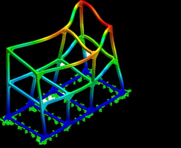
130 Appendix B - Modes Shapes 1st 2nd 3rd 4th 5th 123