8. Issues with Bases

Transcription

1 8. Issues with Bases Nnparametric regressin ften tries t fit a mdel f the frm f(x) = M j=1 β j h j (x) + ǫ where the h j functins may pick ut specific cmpnents f x (multiple linear regressin), r be pwers f cmpnents f x (plynmial regressin), r be prespecified transfrmatins f cmpnents f x (nnlinear regressin). Many functins f cannt be represented by the kinds f h j listed abve. But if the set {h j } is an rthgnal basis fr a space f functins that cntains f, then we can explit many standard strategies frm linear regressin. 1

2 8.1 Hilbert Spaces Usually we are cncerned with spaces f functins such as L 2 [a, b], the Hilbert space f all real-valued functins defined n the interval [a, b] that are square-integrable: b a f(x) dx <. This definitin extends t functins n IR p. Hilbert spaces have an inner prduct. Fr L 2 [a, b] it is < f, g >= b a f(x)g(x) dx. The inner prduct defines a nrm f, given by < f, g > 1/2, which is essentially a metric n the space f functins. There are additinal issues fr a Hilbert space, such as cmpleteness (i.e., the space cntains the limit f all Cauchy sequences), but we can ignre thse. 2

3 A set f functins {h j } in a Hilbert space is mutually rthgnal if fr all j k, < h j, h k >= 0. Additinally, if h j = 1 fr all j, then the set is rthnrmal. If {h j } is an rthnrmal basis fr a space H then every functin f H can be uniquely written as: f(x) = β j h j (x) j=1 where β j =< f, h j >. Sme famus rthgnal bases include the Furier bases, cnsisting f {cs nx, sin nx}, wavelets, Legendre plynmials, and Hermite plynmials. 3

4 If ne has an rthnrmal basis fr the space in which f lives, then several nice things happen: 1. Since f is a linear functin f the basis elements, then simple regressin methds allw us t estimate the cefficients β j. 2. Since the basis is rthgnal, the estimates f different β j cefficients are independent. 3. Since the set is a basis, there is n identifiability prblem; each functin in H is uniquely expressed as a weighted sum f basis elements. But nt all rthnrmal bases are equally gd. If ne can find a basis that includes f itself, that wuld be ideal. Secnd best is a basis in which nly a few elements in the representatin f f have nn-zer cefficients. But this prblem is tautlgical since we d nt knw f. 4

5 One apprach t chsing a basis is t use Gram-Schmidt rthgnalizatin t cnstruct a basis set such that the first few elements crrespnd t the kinds f functins that statisticians expect t encunter. This apprach is ften practical if the right kind f dmain knwledge is available. This is ften the case in audi signal prcessing; Furier series are natural ways t represent vibratin. But in general, ne must pick basis set withut regard t f. A cmmn criterin is that the influence f the basis elements be lcal. Frm this standpint, plynmials and trignmetric functins are bad, because their supprt is the whle line, but splines and wavelets are gd, because their supprt is essentially cmpact. 5

6 Given an rthnrmal basis, ne can try estimating all f the {β j }. But ne quickly runs ut f data even if f is exactly equal t ne f the basis elements, nise ensures that all f the ther elements will make sme cntributin t the fit. T address this prblem ne can: Restrict the set f functins, s it is n lnger a basis (e.g., linear regressin); select nly thse basis elements that seem t cntribute significantly t the fit f the mdel (e.g., variable selectin methds, r greedy fitters like MARS, CART, and bsting); regularize, t restrict the values f the cefficients (e.g., thrugh ridge regressin r shrinkage r theshlding). The first technique is prblematic, especially since it prevents flexiblity in fitting nnlinear functins. The secnd technique is imprtant, especially when ne has large p but small n. But it is ften insufficient, and the thery fr aggressive variable selectin is nt well-develped yet. 6

7 º¾ Ë Ñ Ø Ó Ø Ú ÓÖ Ó Ò Ú Ö Ò º ÙÖ ÑÓ Ð Ô Ø Ø Ó ÐÐ ÔÓ Ð ÔÖ Ø ÓÒ ÖÓÑ Ø Ì Ì ÖÓÑ Ø ØÖÙØ ÓÛÒ ÐÓÒ Û Ø Ø Ú Ö Ò ÑÓ Ð Ý Ø Ð Ö Ý ÐÐÓÛ ÖÐ ÒØ Ö Ø Ø Ð ÓØ Ò Ø ÐÓ Ø Ø Ò ÔÓÔÙÐ Ø ÓÒ º ÖÙÒ Ò ÓÖ Ö ÙÐ Ö¹ Ð ÐÐ Ø Ð Ó ÓÛÒ Ú Ò Ø ÓÒ Ð Ø Ñ Ø ÓÒ ÙØ Þ ÔÖ Ø ÓÒ ÖÖÓÖ Ù ØÓ Ø Ö Ú Ö Ò º Ñ ÐÐ Ö Ð Ñ ÒØ Ó ËØ Ø Ø Ð Ä ÖÒ Ò À Ø Ì Ö Ò ² Ö Ñ Ò ¾¼¼½ ÔØ Ö Realizatin Clsest fit in ppulatin Clsest fit Truth Mdel bias Estimatin Bias MODEL SPACE Shrunken fit Estimatin Variance RESTRICTED MODEL SPACE ÑÓ Ð Û Ø Ø ÐÓ Ø Ø Ð Ð Û Ø Ð Óغ 7

8 8.2 Ridge Regressin Ridge regressin is an ld idea, used riginally t prtect against multicllinearity. It shrinks the cefficients in a regressin twards zer (and each ther) by impsing a penalty n the sum f the squares f the cefficients. ˆβ = argmin β { n (y I β 0 p β j x ij ) 2 + λ p β 2 j } I=1 j=1 j=1 where λ 0 is a penalty parameter that cntrls the amunt f shrinkage. Recall Stein s result that when estimating a multivariate nrmal mean with squared errr lss, the sample average is inadmissible and can be imprved by shinking the estimatr twards 0 (r any ther value). Neural net methds nw ften d similar shrinkage n the weights at each nde, Thereby imprving predictive squared accuracy. 8

9 Ð Ñ ÒØ Ó ËØ Ø Ø Ð Ä ÖÒ Ò À Ø Ì Ö Ò ² Ö Ñ Ò ¾¼¼½ ÔØ Ö Largest Principal Cmpnent Smallest Principal Cmpnent ÈË Ö Ö ÔÐ Ñ ÒØ ½ ¾ ÙÖ º ÈÖ Ò Ô Ð ÓÑÔÓÒ ÒØ Ó ÓÑ ÒÔÙØ Ø ÔÓ ÒØ º Ì Ð Ö Ø ÔÖ Ò Ô Ð ÓÑÔÓÒ ÒØ Ø Ö ¹ Ø ÓÒ Ø Ø Ñ Ü Ñ Þ Ø Ú Ö Ò Ó Ø ÔÖÓ Ø Ø Ò Ø Ñ ÐÐ Ø ÔÖ Ò Ô Ð ÓÑÔÓÒ ÒØ Ñ Ò Ñ Þ Ø Ø Ú Ö Ò º Ê Ö Ö ÓÒ ÔÖÓ Ø Ý ÓÒØÓ Ø Óѹ ÔÓÒ ÒØ Ò Ø Ò Ö Ò Ø Ó Æ ÒØ Ó Ø ÐÓÛ¹ Ú Ö Ò ÓÑÔÓÒ ÒØ ÑÓÖ Ø Ò Ø ¹Ú Ö Ò Óѹ ÔÓÒ ÒØ º 9

10 Ridge regressin methds are nt equivariant under scaling, s ne nrmally standardizes the x ij sample values wrt j s that each has unit variance. Traditinal ridge regressin slves ˆβ = (X X + λi) 1 X y s the name derives frm the stabilizatin f the inverse matrix btained by adding a cnstant t the diagnal. Nte that this increases the trace f the hat matrix, which crrespnds t the degrees f freedm used in fitting the mdel. Ridge regressin (and shrinkage methds in general) can als be btained as the Bayesian psterir mde fr a suitable prir. In the multivariate nrmal case, the prir assumes independent nrmal distributins fr each β j, with cmmn variance. 10

11 Ð Ñ ÒØ Ó ËØ Ø Ø Ð Ä ÖÒ Ò À Ø Ì Ö Ò ² Ö Ñ Ò ¾¼¼½ ÔØ Ö Cefficients lcavl lweight age lbph svi lcp gleasn pgg45 ÈË Ö Ö ÔÐ Ñ ÒØ µ ÙÖ º ÈÖÓ Ð Ó Ö Ó Æ ÒØ ÓÖ Ø ÔÖÓ Ø Ø Ò Ö Ü ÑÔÐ ØÙÒ Ò Ô Ö Ñ Ø Ö Ú Ö¹ º Ó Æ ÒØ Ö ÔÐÓØØ Ú Ö Ù µ Ø «¹ Ø Ú Ö Ó Ö ÓѺ Ú ÖØ Ð Ð Ò Ö ÛÒ Ø ½ Ø Ú ÐÙ Ó Ò Ý ÖÓ ¹Ú Ð Ø ÓÒº 11

12 8.3 The Lass The Lass methd is analgus t ridge regressin. The Lass estimate is given by ˆβ = argmin β { n (y I β 0 I=1 subject t the cnstraint that p j=1 β j s. p j=1 β j x ij ) 2 } The Lass replaces the quadratic penalty in ridge regressin by a penalty n the sum f the abslute values f the β j terms. If s is larger than the sum f the abslute values f the least squares estimatrs, then the Lass agrees with OLS. If s is small, then many f the β j terms are driven t 0, s it is perfrming variable selectin. 12

13 The Lass crrespnds t a Bayesian methd in which the prir n each parameter is Laplacian. 13

14 Ð Ñ ÒØ Ó ËØ Ø Ø Ð Ä ÖÒ Ò À Ø Ì Ö Ò ² Ö Ñ Ò ¾¼¼½ ÔØ Ö Cefficients lcavl lweight lbph svi pgg45 gleasn age lcp Shrinkage Factr s ÙÖ º ÈÖÓ Ð Ó Ð Ó Ó Æ ÒØ ØÙÒ Ò Ô Ö Ñ Ø Ö Ø Ú Ö º Ó Æ ÒØ Ö ÔÐÓØØ Ú Ö Ù Ø È Ô ½ º Ú ÖØ Ð Ð Ò Ö ÛÒ Ø ¼ Ø Ú ÐÙ Ó Ò Ý ÖÓ ¹Ú Ð Ø ÓÒº ÓÑÔ Ö ÙÖ º ÓÒ Ô Ø Ð Ó ÔÖÓ Ð Ø Þ ÖÓ Û Ð Ø Ó ÓÖ Ö Ó ÒÓغ 14

15 Ð Ñ ÒØ Ó ËØ Ø Ø Ð Ä ÖÒ Ò À Ø Ì Ö Ò ² Ö Ñ Ò ¾¼¼½ ÔØ Ö Residual Sum-f-Squares Subset Size k ÙÖ º ÐÐ ÔÓ Ð Ù Ø ÑÓ Ð ÓÖ Ø ÔÖÓ Ø Ø Ò Ö Ü ÑÔÐ º Ø Ù Ø Þ ÓÛÒ Ø Ö ¹ Ù Ð ÙÑ¹Ó ¹ ÕÙ Ö ÓÖ ÑÓ Ð Ó Ø Ø Þ º 15

16 8.4 LARS LARS was intrduced in 2003 ( Least Angle Regressin, Efrn, Hastie, Jhnstne, and Tibshirani, Annals f Statistics). It is clsely related the the Lass and frward stagewise mdeling (the strategy that generated the bsting algrithm). LARS was mtivated by cnsideratin f Frward Selectin in multiple linear regressin. Recall that Frward selectin starts with n variables in the mdel, then adds the variable that best predicts the respnse. It then lks at the residuals frm that fit, and adds the variable that best predicts thse residuals. The prcess cntinues until n remaining variable is significantly assciated with the residuals. 16

17 Ý Ö ÔÖ ÒØ Ø Ú ØÓÖ Ó Ø Ð Ø ÕÙ Ö ÔÖ Ø ÓÒ Ü ¾ Ü ½ Ð Ñ ÒØ Ó ËØ Ø Ø Ð Ä ÖÒ Ò À Ø Ì Ö Ò ² Ö Ñ Ò ¾¼¼½ ÔØ Ö ÈË Ö Ö ÔÐ Ñ ÒØ Ý Ý ÙÖ º¾ Ì Æ ¹ Ñ Ò ÓÒ Ð ÓÑ ØÖÝ Ó Ð Ø ÕÙ Ö Ö Ö ÓÒ Û Ø ØÛÓ ÔÖ ØÓÖ º Ì ÓÙØÓÑ Ú ØÓÖ Ý ÓÖØ Ó ÓÒ ÐÐÝ ÔÖÓ Ø ÓÒØÓ Ø ÝÔ ÖÔÐ Ò Ô ÒÒ Ý Ø ÒÔÙØ Ú ØÓÖ Ü ½ Ò Ü ¾º Ì ÔÖÓ Ø ÓÒ The gemetry f regressin is key. Nte that linear regressin estimates β by prjecting the Y nt the subspace spanned by the explanatry variables: ˆβ = (X X) 1 X Y s Ŷ = HY = X(X X) 1 X Y. Here H (the hat matrix ) is a prjectin matrix. See Christiansen (1987) fr details. 17

18 The LARS strategy starts with all ˆβ cefficients equal t zer. It then takes the largest step pssible in the directin f the predictr mst crrelated with Y. The step ends when sme ther predictr has as much crrelatin with the current residual. LARS then steps in the directin that bisects the angle between the tw mst-crrelated predictrs, and cntinues until a third variable becmes as crrelated with the residuals as the first tw. LARS then mves equiangularly between thse three variables, and s n. LARS differs frm Frward Selectin in that at the end f the first step, Frward Selectin wuld cntinue t mve in the directin f the first predictr, until the crrelatin between it and the current residuals was reduced t zer. LARS is clsely related t the LASSO and t Frward Stagewise mdeling, althugh this is nt bvius. 18

19 The LARS algrithm fr p = 2 predictrs. The ȳ 2 is the prjectin f y n the space spanned by x 1 and x 2, the clumns f the X matrix. The LARS predictin at step k is ˆµ k = X ˆβ L k where ˆβ L k is the LARS estimate at step k. 19

20 Beginning at µ 0 = 0, the residual vectr ȳ ˆµ 0 has larger crrelatin with x 1 than x 2. S LARS steps in the directin f x 1 as far as it can until the current residuals are as crrelated with x 2 as with x 1. That first step gives tw estimates, ˆµ 1 and, implicitly, ˆβ L 1. Here ˆµ 1 = ˆµ 0 + ˆγ 1 x 1 where ˆγ 1 is chsen s that ȳ 2 ˆµ 1 bisects the angle between x 1 and x 2. The secnd step mves alng the unit vectr u 2 that bisects the angle. It ges distance ˆγ 2, and terminates at the OLS estimatr ȳ 2. 20

21 Sme cmments: Fr p explantry variables, the LARS estimate arrives at the OLS estimate n step p. The Frward Selectin algrithm wuld, n the first step, prceed alng the x 1 directin until it reaches the prjectin f ȳ 2 nt the x 1 subspace at ȳ 1, as shwn n the graph. A Stagewise selectin prcedure fits at each step a mdel that imprves, in ne variable, the fit. This is shwn by the staircase in the figure. It necessarily takes small steps, and thus is cmputatinally intensive. If tw predictrs are perfectly crrelated, LARS wuld use bth and put equal weight upn them. The Lass can be btained as a slight mdificatin f the LARS algrithm (see sectin 3.1 in the Efrn et al. paper). LARS, the Lass, and Frward Stagewise regressin give very similar answers. 21

22 Lass and Stagewise regressin estimates fr the diabetes study. Nte that bth are autmatically parsimnius. 22

23 LARS regressin estimates fr the diabetes study. Nte that it is als autmatically parsimnius. 23

24 8.5 Bayesian Methds Suppse there are p explanatry variables and ne cnsiders a mdel f the frm: M i : Y = X i β i + ǫ where ǫ N(0, σ 2 I) and i = 1,...,2 p, indexing all pssible chices f inclusin r exclusin amng the p explanatry variables. Assume there is an intercept: each β i = (β 0, β i ), and thus let X i be the submatrix f X i crrespnding t β i, and let the length f β i be d(i) + 1. Dente the density crrespnding t mdel M i by f i (y β i, σ 2 ). 24

25 Fr this mdel, standard chices fr the prir n the parameters in M i include: The g-prirs. Here: π g i (β i, σ 2 ) = 1 σ 2 N(β i 0, cnσ 2 (X i X i) 1 ) where c is fixed (typically t 1, r estimated thrugh empirical Bayes). Zellner-Siw prirs. The intercept mdel has prir π(β 0, σ 2 ) = 1/σ 2, while the prir fr all ther M i is: π ZS i (β i, σ 2 ) = π g i (β i, σ 2 c) π ZS i (c) InverseGamma(c 0.5, 0.5). The marginal density under M i is m i (Y ) = f i (y β i, σ 2 )π(β i, σ 2 )dβ i dσ 2. 25

26 If all mdels M i have equal prir prbability, then the psterir prbability f a mdel is P(M i Y ) = m i(y) k m k(y ). Recall the psterir inclusin prbability fr the ith variable: q i = P(β i crrect mdel Y ) = k P(M k Y )I βi M k. The median prbability mdel is the mdel cnsisting f all and nly thse variables whse psterir inclusin prbability is at least 1/2. 26

27 Usually, the median prbability mdel is superir t the maximum psterir prbability mdel fr predictin. (But the Bayesian mdel average is better than bth, if ne can use an ensemble methd.) Therem: (Barbieri and Berger, 2004, Annals f Statistics. Cnsider a sequence f nested linear mdels. If predictin is wanted at future cvariates like the past, the psterir mean under M i satisfies β i = bˆβ i, where ˆβ i is the OLS estimate, then the best single mdel fr predictin under squared errr lss is the median prbability mdel. The secnd cnditin is satisfied if ne uses either nninfrmative prirs fr the mdel parameters r if ne uses g-type prirs with the same cnstant c > 0 fr each mdel (and any prir n σ 2 ). 27

28 Example: Plynmial regressin. Here M i is y = i j=0 β j x j + ǫ. Mdel P(M i Y ) Cvariate j P( x j is in mdel Y ) The crrect mdel was M 3, which is the median prbability mdel. But the MAP mdel is M 4. 28

29 8.6 Overcmpleteness Statisticians traditinally have used an rthgnal basis f functins {h j } fr estimating functins f: M ˆf(x) = ˆβ j h j (x). j=1 This chice is largely mtivated by the independence f the cefficient estimates and the ability t d asympttic thery. But cmputer scientists have fund that using larger sets f functins than are available in the rthgnal basis can imprve perfrmance. See Wlfe, Gdsill, and Ng (2004; Jurnal f the Ryal Statistical Sciety, Series B, 66, 1-15). 29

30 This larger set is called a frame. A frame cntains a basis fr the space f interest (e.g., L 2 [a, b]), but may als ther functins. Frmally, a frame is a set f functins {h j : j J} with the prperty that there are cnstants A, B > 0 such that A f 2 j J < f, h j > 2 B f 2 f H. A frame that is just an rdinary basis has A = B = 1. A frame that is the unin f tw rdinary bases has A = B = 2. Sme frames have uncuntable cardinality. Nntrivial frames cntain at least ne nn-zer element which can be written as a linear cmbinatin f the ther elements in the frame. This cntrasts with the situatin fr basis sets. The advantage f frames is that their greater size allws the pssibility f finding a very parsimnius representatin fr f. 30

31 One wants a criterin fr cmparing the perfrmance f different frames used fr functin estimatin. Cnsider estimating functins in L 2 [a, b]. If ne frms an vercmplete frame as the unin f tw basis sets, is it better t take the unin f a Furier basis and a Hermite plynmial basis, r the unin f a Furier basis and the Haar basis? One imagines that it wuld be desirable t cmbine bases that cntain very different functins. Frm this perspective, the Furier basis, which is smth, might be mre effectively cmbined with the rugh Haar basis than the smth Hermite plynmial basis. Thus the resulting frame wuld cntain elements that allw parsimnius representatin f bth smth and rugh functins. The fllwing figure shws the first tw elements f these three bases. 31

32 32

33 One prpsal fr a criterin that cmpares tw frames depends upn the parsimny f the apprximating functins. Fr a given frame F = { h j : j J }, a functin f, and a tlerance ǫ, cnsider the set f all apprximating functins S(f, ǫ ) = { ˆf : ˆf = k β j h j and f ˆf < ǫ }. j=1 Each ˆf S(f, ǫ ) has a certain number f terms in the sum. The mst parsimnius apprximatin is the ne that uses the fewest terms h j. Let k(f, ǫ ) = inf{j : ˆf S(f, ǫ )}. Sme functins f L 2 [0, 1] will be hard t apprximate with elements in the frame F, and fr these functins k(f, ǫ ) will be large (and maybe infinite). 33

34 T handle the wrst case fr estimatin, let k(ǫ ) = sup { k(f, ǫ ) }. f L 2 [0,1] This is the number f terms needed t apprximate the mst difficult functin in L 2 [0, 1] t within ǫ using nly frame elements. Fr sme frames and values ǫ, k(ǫ ) will be infinite. But there are many cases in which it is finite. Fr example, if F cntains an ǫ -net, this trivially ensures that k(ǫ ) = 1. Fr nn-trivial cases in which frames F and G are unins f bases, ne wuld like t say that frame F is better than frame G at level ǫ if k F (ǫ ) < k G (ǫ ), where the subscript indicates the frame. If there exists sme γ such that the inequality hlds fr all ǫ < γ, then ne culd bradly claim that F is better than G. 34

35 9. Wavelets A wavelet is a functin that lks like a lcalized wiggle. Special cllectins f wavelets can be used t btain apprximatins f functins by separating then infrmatin at different scales. The stunning success f wavelets has spurred explsive grwth in research. Dnh and Jhnstne (1994; Bimetrika, 81, ) led the way in statistics, shwing that wavelets can achieve lcal asympttic minimaxity in apprximating thick classes f functins. Lcal asympttic minimaxity is a technical prperty, but it ensures that the estimates are asympttically minimax with respect t a large family f lss functins in a large class f functins. Such estimates prbably evade the COD, in the same technical sense that neural nets d. 35

36 In its simplest frm, a wavelet representatin begins with a single functin ψ, ften called th mther wavelet. We define a cllectin f wavelets called a wavelet basis by dilatin and translatin f the mther wavelet ψ: fr j, k Z, the set f integers. ψ jk (t) = 2 j/2 ψ(2 j t k) One btains an vercmplete frame if ne allws j, k t take values in IR rather than Z. This is called an undecimated wavelet basis. Each ψ jk has a characteristic reslutin scale (determined by j) and is rughly centered n the lcatin k/2 j. It turns ut that if ψ is prperly chsen, any reasnable functin can be represented by an infinite linear cmbinatin f the ψ jk functins. 36

37 Wavelets have three key features: Wavelets prvide sparse representatins f a brad class f functins and signals, Wavelets can achieve very gd lcalizatin in bth time and frequency, There are fast algrithms fr cmputing wavelet representatins in practice. Sparsity means that mst f cefficients in the linear cmbinatin are nearly zer. A single wavelet basis can prvide sparse representatins f many spaces f functins at the same time. Gd lcalizatin means that bth the wavelet functin ψ and its Furier transfrm have small supprt; i.e., the functins are essentially zer utside sme cmpact dmain. Regarding speed, wavelet representatins can be cmputed in O(n lg n) and smetimes O(n) peratins (the FFT is O(n lg n)). 37

38 9.1 Cnstructing Wavelets We begin with a mathematical descriptin f a smth lcalized wiggle. Let L p (IR) dente the space f measurable cmplex-valued functins f n the real numbers IR such that [ ] 1/p f p = f(x) p dx <. Here L 2 (IR) is a Hilbert space with inner prduct defined by < f, g >= f(x)ḡ(x) dx, where ḡ is the cmplex cnjugate f g. Recall that a cmplex functin g(x) = u(x) + iv(x) has cnjugate ḡ(x) = u(x) iv(x) where u(x) and v(x) are real-valued functins and i is 1. The mdulus f g(x) is u2 (x) + v 2 (x). 38

39 Fr integers D, M 0, suppse that ψ L 2 (IR) satisfies the fllwing fr d = 0,...,D and m = 0,...,M: 1. The derivative ψ (d) exists and is in L (IR), 2. The mdulus ψ (d) is rapidly decreasing as x, and 3. The mth mment f ψ vanishes, i.e., x m ψ(x) dt = 0. Then we say that ψ is a basic wavelet f regularity (D, M). Cnditin 1 implies that ψ is smth, and cnditins 1 and 2 tgether imply that ψ is lcalized in time and frequency. Cnditin 2 implies that ψ is highly cncentrated in the x dmain by requiring that it decrease faster than any inverse plynmial utside sme cmpact set. Cnditin 1 implies that the Furier transfrm f ψ is quite cncentrated as well, decreasing faster than the reciprcal f a D-degree plynmial fr high frequency. Cnditin 3 frces ψ t be wiggly since the integral f ψ with any plynmial up t degree M must be zer. 39

40 The standard example f a wavelet basis is the Haar Basis. Let ψ = 1 [0,1/2) 1 [1/2,1) where 1 A is the indicatr functin f the set A. Then the mther wavelet is: 40

41 This functin is nt differentiable, but it has cmpact supprt and integrates any cnstant t zer. Thus ψ is a basic wavelet f regularity (0, 0). If we define ψ jk frm ψ by translatin and dilatin, we btain a dubly-infinite set f functins with the same prperties as ψ. Mrever, any tw ψ jk are rthnrmal in the sense that < ψ j,k, ψ j,k >= δ jj δ kk where δ is a Krnecker delta. These ψ jk frm an rthnrmal basis fr L 2 (IR). any functin in L 2 (IR) can be well-apprximated by j,k β j,kψ jk. (As a first step in seeing this, nte that it is sufficient t be able t apprximate any functin that is piecewise cnstant n dyadic intervals.) 41

42 Since the Haar basis cnsists f step functins, an apprximatin f a smth functin by a finite number f Haar wavelets is necessarily ragged. The cnstructin f smther variants f the Haar basis leads t mre general wavelets. 42

43 A wavelet basis is especially useful if it can extract interpretable infrmatin abut f L 2 (IR) thrugh the inner prduct β =< f, ψ >. If ψ is well-lcalized in IR, then a β cefficient essentially reflects the behavir f f n a particular part f its dmain (unlike the case in linear regressin). Similarly, if ψ is well-lcalized in frequency, then β essentially reflects particular frequency cmpnents f f as well. Suppse that ψ is cncentrated in a small interval and that in that interval f can be apprximated by a Taylr series; then, since the inner prduct with ψ cancels all plynmials up t degree M, β reflects nly the higher-rder behavir in f. (Anther way t state this is that if tw functins differ nly by a plynmial f degree M r smaller, their β cefficient will be the same.) 43

44 Fr a basis {ψ jk }, the index j represents reslutin scale; as j increases, ψ jk becmes cncentrated in a decreasing set. The index k represents lcatin; as k changes, the functin is shifted alng the line. Hence, the map (j, k) β j,k =< f, ψ jk > prvides infrmatin abut f at every dyadic scale and lcatin. The wavelet representatin f(x) = j Z k Z β jk ψ jk (x) is called the hmgenus equatin. It expresses f in terms f functins that all integrate t 0. (There is n paradx here, since cnvergence in L 2 (IR) and cnvergence in L 1 (IR) are nt the same thing.) 44

45 9.2 The Father Wavelet It is ften useful t re-express the hmgenus equatin in an equivalent but inhmgenus frm. This frm separates carse structure frm fine structure. T d this, select a cnvenient reslutin level J 0. Reslutin levels j J 0 capture the carse structure f f and levels j > J 0 capture the fine structure. One apprximates the fine-reslutin structure f f by a linear cmbinatin f the ψ jk at j J 0, and ne apprximates the carse-reslutin structure by a cmbinatin f the functins φ k (t) = φ(t k) fr k Z, where φ is called the father wavelet(r scaling functin). The inhmgenus representatin fr f L 2 (IR) is then f = < f, φ k > φ k + < f, ψ jk > ψ jk. k Z j J 0 k Z 45

46 This father wavelet φ is clsely related t the mther wavelet ψ: ne can chse φ s that < φ, ψ >= 0, the father wavelet satisfies the first tw requirements f a basic wavelet with the same indices f regularity as ψ. The difference between the inhmgenus and hmgenus representatins lie in the first sum. This aggregates the infrmatin in the lw reslutin levels thrugh the specially cnstructed functin φ rather than distributing it amng the ψ jk terms. The prime advantage f this inhmgenus representatin is that the carse/fine dichtmy is intuitively appealing and useful. This is especially the case if the nise in the functin estimatin can be thught f as high-frequency, while the signal in the prblem is lw-frequency. 46

47 Fr the Haar Basis, the father wavelet is the indicatr f the unit interval, φ = 1 [0,1). When J 0 = 0, the inhmgenus representatin takes the frm f = α k φ k + β j,k ψ jk, k Z j 0 k Z where α k =< f, φ k > and β j,k =< f, ψ jk >. The cefficients α k are just integrals f f ver intervals f the frm [k, k + 1); the remaining structure in f is represented as fluctuatins within thse intervals. Nte that φ is in L 2 (IR), and cnsequently can be written in terms f the ψ jk : φ = 1 2 ψ 1, j/2 ψ j,0. j=2 This uses nly the carsest ψ jk terms, as expected. The relatinship between ψ and φ ges the ther way as well: ψ = 1 [0,1/2) 1 [1/2,1) by definitin, which is a linear cmbinatin f translated and dilated φ terms. 47

48 9.3 Multireslutin Analysis A key idea in wavelets is that f successive refinement. If ne can apprximate at several levels f accuracy, then the differences between successive apprximatins characterize the refinements needed t mve frm ne level t anther. Multireslutin analysis (MRA) frmalizes this ntin fr apprximatins that are related by a translatin and dilatin. An MRA is a sequence f nested apprximatin spaces fr a cntaining class f functins. Fr the cntaining class L 2 (IR), MRA is a nested sequence f clsed subspaces V 2 V 1 V 0 V 1 V 2 such that 1. cls { j Z V j } = L 2 (IR) 3. f V j f(2 j ) V 0 j Z 2. j Z V j = {0} 4. f V 0 f( k) V 0 k Z. 48

49 Cnditin 1 ensures that the apprximatin spaces (V j ) are sufficient t apprximate any functin in L 2 (IR). There are many sequences f spaces satisfying Cnditins 1, 2 and 4; the name multireslutin is derived frm Cnditin 3 which implies that all the V j are dyadically scaled versins f a cmmn space V 0. By Cnditin 4, V 0 is invariant under integer translatins. When generating rthnrmal wavelet bases, we als require that the space V 0 f the MRA cntains a functin φ such that the integer translatins {φ 0,n } frm an rthnrmal basis fr V 0. Fr simplicity, we will fcus almst exclusively n rthnrmal bases here. 49

50 Since V 0 V 1, we can define its rthgnal cmplement W 0 in V 1, s V 1 = V 0 W 0. We can d likewise fr every j, where V j+1 = V j W j. The sequence f spaces {W j } j Z are mutually rthgnal and they are inherit Cnditin 3 frm the V j ; i.e., f W j if and nly if f(2 j ) W 0. By themselves, these spaces prvide a hmgeneus representatin f L 2 (IR), since L 2 (IR) = cls{ j Z W j}. The W j are the building blcks fr successive refinement frm ne apprximating space t anther. Given f L 2 (IR), the best apprximatin t f in any V j is given by P j f, where P j is the rthgnal prjectin nt V j. It fllws that Q j = P j P j 1 is the rthgnal prjectin nt W j. 50

51 Given a carse apprximatin P 0 f, ne can refine t the finer apprximatin P J f fr any J > 0 by adding details frm successive W j spaces: P J f = P 0 f + = P 0 f + J P j f P j 1 f j=1 J 1 j=0 Q j f, and as J, f = P 0 f + Q j f. j=0 Successive refinement exactly mimics the inhmgenus wavelet representatin. The carse apprximatin P 0 f crrespnds t a linear cmbinatin f the φ 0,k, and each Q j f fr j 0 crrespnds t a linear cmbinatin f the span f the ψ jk. 51

52 As an example, suppse V j is the set f piecewise cnstant functins n intervals f the frm [k2 j, (k + 1)2 j ). S V 0 is generated by integer translatins f the functin φ = 1 [0,1), the father wavelet fr the Haar basis. Fr f L 2 (IR), let α j,k =< φ j,k, f >. Then P 0 f = k α 0,kφ 0,k and P 1 f = k α 1,kφ 1,k are apprximatins t f that are piecewise cnstant n unit and half-unit intervals, respectively. Hw des ne refine the carse apprximatin P 0 f t the next higher reslutin level? We knw α 0,k = 1 2 (α 1,2k + α 1,2k+1 ), but we als need t knw the difference β 0,k = 1 2 (α 1,2k α 1,2k+1 ) between the integrals f f ver the half-intervals [k, k + 1/2) and [k + 1/2, k + 1). This β 0,k is just the cefficient < ψ 0,k, f > f the (0, k) Haar wavelet ψ 0,k. The translatins f the Haar mther wavelet frm an rthnrmal basis fr the space W 0. 52

53 Fr a general MRA, hw des ne find the crrespnding ψ? It turns ut that ψ and φ determine each ther thrugh the refinement relatins amng the spaces. S ne can cnstruct a functin ψ whse integer translatins (i.e., ψ 0,k (t) = ψ(t k)) yield an rthnrmal basis f W 0. By cnstructin, bth ψ and φ are in V 1, and the ψ 0,k and φ 0,n are rthgnal. It fllws that bth φ and ψ can be expressed as a linear cmbinatin f the φ 1,n with sme cnstraints n the cefficients. This reasning leads t the fllwing tw-scale identities: φ(t) = 2 n ψ(t) = 2 n g n φ(2t n) h n φ(2t n). The {h n } and {g n } satisfy n h n 2 = 1 and n g n 2 = 1. Orthgnality f the φ k (t) and ψ 0,k and the fact that V 1 is a direct sum f V 0 and W 0 frce relatinships amng {g n } and {h n }. 53

54 Fr a specific MRA, these relatinships prvide enugh cnditins t uniquely identify mther and father wavelets φ and ψ. In the Haar case, the sequences are {g n } = (...,0, 1/ 2, 1/ 2, 0,...) {h n } = (...,0, 1/ 2, 1/ 2, 0,...). In general, it is mre cnvenient t wrk with the tw-scale identities in the Furier dmain s as t characterize the Furier transfrms φ and ψ. The value f the tw-scale identities is in the cnnectins they imppse n the wavelet cefficients. By the tw-scale identities, φ jk (t) = 2 (j+1)/2 n g n φ(2 j+1 t 2k n) ψ jk (t) = 2 (j+1)/2 n h n φ(2 j+1 t 2k n). 54

55 It fllws that < φ jk, f > = n = n g n < φ j+1,2k+n, f > g n 2k < φ j+1,n, f > and < ψ jk, f > = n = n h n < φ j+1,2k+n, f > h n 2k < φ j+1,n, f >. Each results frm cnvlving the sequence f higher-reslutin inner prducts with the reversed sequences {g n } and {h n } and then retaining nly the even numbered cmpnents f the cnvlutin. S given the cefficients < φ J,k, f > fr k Z at sme fixed reslutin level J, ne can cmpute the cefficients at all carser levels by successively filtering and decimating the sequences. This is the heart f the Discrete Wavelet Transfrm (DWT). 55

56 10. Cluster Analysis In data mining, cluster analysis is ften called structure discvery. Traditinal data methds attempt t cluster all f the cases, but in data mining is is ften sufficient t just find sme f the clusters. Recent applicatins include: market segmentatin (e.g., Claritas, Inc.) syndrmic surveillance text retrieval micrarray data 56

57 Classical statistics invented three kinds f cluster analysis, many f which were independently reinvented by cmputer scientists. These three families are: hierarchical agglmerative clustering, which develped in the bilgical sciences and is the mst widely used strategy; k-means clustering, which is an algrithmic technique invented by MacQueen (1967; Prceedings f the Fifth Berkeley Sympsium n Mathematical Statistics and Prbability, University f Califrnia Press, ); mixture mdels, which were recently prpsed by Banfield and Raftery (1993; Bimetrics, 49, ) and are gaining wide currency. Of these three methds mixture mdels make the strngest assumptins abut the data being a randm sample frm a ppulatin, but this is als the methd which best supprts inference. 57

58 10.1 Hierarchical Clustering Hierarchical agglmerative clustering jins cases tgether accrding t a fixed set f rules. 0. One starts with a sample x 1,..., x n f cases and a metric d n all pssible sets f cases (including the singletn sets). 1. At the first step, ne jins the tw cases x i and x j that have the minimum distances amng all pssible pairs f cases. 2. At the secnd step, ne jins either tw singletn cases r a case x k t {x i, x j }, accrding t whichever situatin achieves minimum distance. 3. At subsequent steps ne may be jining either pairs f cases, pairs f sets f cases, r a case t a set. Sibsn and Jardine (1971; Mathematical Taxnmy, Wiley) shw that this apprach uniquely satisfies certain theretically desirable prperties. 58

59 The result f a hierarchical agglmerative cluster analysis is ften displayed as a tree. The lengths f the edges in the binary tree shws the rder in which cases r sets were jined tgether and the magnitude f the distance between them. But it is hard t knw when t stp grwing a tree and declare the clusters. Milligan and Cper (1985; Psychmetrika, 50, ) like the cubic clustering criterin. 59

60 Sme f the classic metrics fr linking sets f cases are: Nearest-neighbr r single linkage. Here ne has a metric d n IR p and defines d(a, B) = min a A,b B d (a, b). Cmplete linkage. Here d(a, B) = max a A,b B d (a, b). Centrid linkage. Here d(a, B) = d (ā, b) where ā is the centrid (r average) f A and b is the centrid f B. Many thers have been used. Ward s metric lks at the rati f between-set and within-set sums f squares, thers use varius kinds f weighting, etc. Fisher and Van Ness (1971; Bimetrika, 58, ) cmpare the prperties f these metrics in a series f papers. 60

61 When the sample size is very large, and r p is large, then the fastest way t cluster cases uses single linkage and creates a minimal spanning tree. Then ne just remves the lngest edges t create clusters, as shwn belw. There is an O(n 2 ) algrithm fr this that was develped by Prim (1957; Bell System Technical Jurnal, 36, ). It can even be accelerated a little bit. 61

62 When p is large and mst f the measurements are nise, then it is very difficult t discver true cluster structure. The signal that distinguishes the clusters gets lst in the chance variatin amng the spurius variables. Graphical methds such as G-Gbi take t lng t find interesting prjectins (via a Hermite plynmial functin that measures interestingness accrding t the gappiness f the prjectin). See Swayne, Ck, and Buja (1998; Jurnal f Cmputatinal and Graphical Statistics, 7, ). Visualizatin techniques prbably becme infeasible fr p > 10 r s. 62

63 Anther thing that can happen with large p is that there are multiple cluster structures. Here cases shw strng clustering with respect t ne subset f variables, and cmparably strng, but distinct, clusters with respect t a different subset f the variables. This situatin gives rise t prduct structure in the clustering, which quickly becmes unmanageable. Friedman and Meulman (2004, Jurnal f the Ryal Statistical Sciety, Series B, t appear) discuss this prblem and related issues. One strategy fr visualizing multiple cluster structure is t use parallel crdinate plts, invented by Inselberg (1985; The Visual Cmputer, 1, 69-91). 63

64 This shws that cases A, B, C and D, E, F have distinct cluster structure with respect t variables x 1, x 2, and x 3, while cases C, E, B and F, A, D Cluster n variables x 6 and x 7. There is n cluster structure n x 4 and x 5. 64

65 10.2 k-means Clustering In k-means clustering the analyst picks the number f clusters k and makes initial guesses abut the cluster centers. The algrithm starts at thse k centers and absrbs nearby cases. Then it calculates a new cluster center (usually the mean) based upn the absrbed cases, and ften a cvariance matrix, and then absrbs mre cases that are nearby, ususually in terms f Mahalanbis distance, t the current center: d(x i, x j ) = [(x i x j ) S 1 (x i x j )] 1/2 where S is the within-cluster cvariance matrix and x j is the center f the current cluster j. The prcess cntinues until all f the cases are assigned t ne f the k clusters. 65

66 Smart cmputer scientists can d k-means clustering (r apprximately this) very quickly. Andrew Mre presented methds at the NSA cnference n streaming data in December As in hierarchical agglmerative clustering, it is hard t knw k. But ne can d univariate search try many values f k, and pick the ne at the knee f sme lack-f-fit curve, e.g., the rati f the average within-cluster t between-cluster sum f squares. The cluster centers mve ver time. If they mve t much, this suggests that the clusters are unstable. N unique slutin is guaranteed fr k-means clustering. In particular, if tw starting pints fall within the same true cluster, then it can be hard t discver new clusters. 66

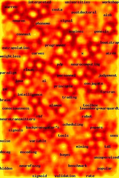
67 Self-Organizing Maps Khnen (1989; Self-Organizatin and Assciative Memry, Springer-Verlag) develped a prcedure called Self-Organizing Maps r SOMs. They quickly becme ppular fr visualizing cmplex data. SOMs have becme widely used in sme aspects f business and infrmatin technlgy, but their underlying thery may be weak. There is n real way t specify uncertainty, and the methd is highly susceptible t utliers. It turns ut that SOMs can be viewed as k-means clustering with the cnstraint that the cluster centers have t lie in a plane. 67

68 SOMs are rather like multidimensinal scaling. The intentin is t prduce a tw-dimensinal (smetimes three-dimensinal) picture f high-dimensinal data, ne that puts similar bservatins clse tgether in the visualizatin. One starts with a set f prttypes, which are just the integer crdinates in the plane frmed by the first tw principal cmpnents f the data. This plane is then distrted, s as t pull the prttypes near t the data. Finally, the data are identified with their nearest pint n the distrted surface. The fllwing tw examples f SOMs are heatmaps shwing the number f dcuments in the newsgrup crpus cmp.ai.neural-nets with different kinds f subject matter, taken frm the WEBSOM hmepage. The first is the entire crpus (with well-ppulated ndes tagged with their keywrd), and the secnd is a blw-up f the heatmap fcused n the regin arund mining. 68

69 69

70 70

71 10.3 Mixture Mdels Mixture mdels fit data by a weighted sum f pdfs: f(x) = k j=1 π j g j (x θ j ) where the π j are psitive and sum t ne and the g j are density functins in a family indexed by θ. The main technical difficulty with mixture mdels is identifiability. Bth Mdel 1 : {π 1 =.5, g 1 = N(0, 1); π 2 =.5, g 2 = N(0, 1)} Mdel 2 : {π 1 = 1, g 1 = N(0, 1); π 2 = 0, g 2 = N( 10, 7)} describe exactly the same situatin. But identifiability is nly an issue at the edges f the mdel space in mst regins it is nt a prblem. 71

72 Bruce Lindsay (1995; Mixture Mdels: Gemetry, Thery, and Applicatins, IMS) gives a cnvexity argument fr slving the identifiability prblem. But this has nt yet wrked its way int data mining practice. Traditinal mixture mdeling ducks the identifiability questin and uses the EM algrithm (cf. Dempster, Laird, and Rubin; 1977, Jurnal f the Ryal Statistical Sciety, Series B, 39, 1-22) fr mdel fitting. T illustrate this, cnsider hw t fit a tw-cmpnent Gaussian mdel t the fllwing smthed histgram. 72

73 The mdel fr an bservatin is f(x) = πφ(x µ 1, σ 2 1) + (1 π)φ 2 (x µ 2, σ 2 2) where φ j is the nrmal density with parameters θ j = (µ j, σ 2 j ). Let θ = (π, µ 1, µ 2, σ1 2, σ2 2 ). A direct effrt t maximize the lg-likelihd leads t n l(θ, x) = ln[πφ 1 (x i µ 1, σ1 2 ) + (1 π)φ 2(x i µ 2, σ2 2 )] i=1 which turns ut t be difficult t slve. The EM algrithm alternates between an expectatin step and a maximizatin step in rder t cnverge n a slutin fr the maximum likelihd estimates in this prblem. 73

74 Instead, assume that there are latent variables (unbserved variables) i that determine frm which mixture cmpnent bservatin x i came. 0 if x i φ 2 i = x 2 2 if x i φ 1 Then we can write the fllwing generative mdel: Y 1i = N(µ 1, σ1) 2 Y 2i = N(µ 2, σ2 2 ) X i = i Y 1i + (1 i )Y 2i where IP[ i = 1] = π. If we knew the { i } then we culd get the mles fr (µ j, σj 2 ) separately fr j = 1, 2, and this wuld be easy. But since we d nt, we use the EM algrithm t btain estimates by iterative alternatin. 74

75 1. Make initial guesses fr ˆπ, ˆµ 1, ˆµ 2, ˆσ 2 1, and ˆσ2 2. Usually we take ˆπ =.5, the ˆµ j are well-separated sample values, and the variance estimates are bth set t the sample variance f the full dataset. 2. Expectatin Step. Cmpute the expected values f the i terms (these are smetimes called respnsibilities ). The respnsibity γ i is: γ i = ˆπφ 1 (x i ˆµ 1, ˆσ 2 1 ) ˆπφ 1 (x i ˆµ 1, ˆσ 2 1 ) + (1 ˆπ)φ 2(x i ˆµ 2, ˆσ 2 2 ). Nte that this is an apprximatin t the psterir prbability the x i cmes frm cmpnent φ Maximizatin Step. Cmpute the new estimates by weighting the sample: ˆµ 1 = n i=1 γ ix i / n i=1 γ i ˆµ 2 = n i=1 (1 γ i)x i / n i=1 (1 γ i) ˆσ 1 2 P = n i=1p γ i(x i ˆµ 1 ) 2 n i=1 γ ˆσ 2 P i 2 = n i=1 P (1 γ i)(x i ˆµ 2 ) 2 n i=1 (1 γ. i) Als, the new ˆπ is n 1 n i=1 γ i. 4. Repeat steps 2 and 3 until cnvergence. 75

76 The EM algrithm climbs hills, s in general it cnverges t a lcal (but pssibly nt glbal) maximum. In part, it is fast because it increases the criterin functin n bth steps, nt just the maximizatin step. The EM algrithm des nt slve the identifiability prblem that can arise in mixture mdels. But it des find a lcal mle. The EM algrithm is cnsiderably mre flexible than this example indicates, and it applies in a wide variety f cases (e.g., imputatin in missing data prblems, inference n causatin thrugh cunterfactual data). The review given here fllws the applicatin in Hastie, Tibshirani, and Friedman (2001; The Elements f Statistical Learning, Wiley, chap. 8.5). 76

77 Mdel-Based Cluster Analysis This is a parametric family f mixture mdels (usually Gaussian mixtures) that are becming widely used in bth cluster analysis and data mining. Essentially, this uses a nested sequence f nrmal mixtures fr cluster analysis. The nesting enables ne t use likelihd rati tests t determine which level f mdeling is apprpriate. 1. At the mst nested level, the mdel assumes that the data cme frm a k-cmpnent mixture f nrmal distributins, each with a cmmn cvariance matrix but different means. 2. At the next-mst nested level, the cvariance matrices are allwed t differ by an unknwn scalar multiple. 3. At the highest level, the cvariance matrices fr different cmpnents are cmpletely unrelated. 77

78 The nesting prblem des nt avid the prblem f identifiability r chice f k. The EM algrithm is used fr estimatin. 78