Multi-Proxy Ostracode Analyses of Paleosalinity in Two Bays, Vieques, Puerto Rico

Transcription

1 Wesleyan University The Honors College Multi-Proxy Ostracode Analyses of Paleosalinity in Two Bays, Vieques, Puerto Rico by Satrio A. Wicaksono Class of 2010 A thesis submitted to the faculty of Wesleyan University in partial fulfillment of the requirements for the Degree of Bachelor of Arts with Departmental Honors in Earth & Environmental Sciences Middletown, Connecticut April, 2010

2 Table of Contents Table of Contents List of Figures and Tables Acknowledgements Abstract i ii iv v 1. Introduction Vieques, Puerto Rico Puerto Mosquito and Puerto Ferro Salinity and paleosalinity Ostracodes Direction and purpose of this study Materials and Methods Background to the Vieques Bioluminescent Bays project Sample Collection Stratigraphy and sedimentology Chronology Grain size analysis Species assemblage analysis Pore morphometric analysis Trace metal geochemistry analysis Bioassemblage Analysis Background Results Discussion Pore Morphometric Analysis Background Results Discussion Trace Metal Geochemistry Analysis Background Results Discussion Synthesis Paleosalinity model Proxy comparison Conclusions and future work 99 References 102 Appendices 112 i

3 List of Figures and Tables Figure 1.1 Google map view of Puerto Rico and Vieques, PR 2 Figure 1.2 Geologic map of Vieques Island 2 Figure 1.3 Google map view of Puerto Mosquito and Puerto Ferro 4 Figure 1.4 Soft body structure of an ostracode 11 Figure 1.5 General anatomy and morphology of an ostracode carapace 12 Figure 2.1 Core locations in PM and PF 18 Figure 2.2 Ideal stratigraphic/sedimentary sequence for PM 19 Figure 2.3 Ideal stratigraphic/sedimentary sequence for PF 20 Figure 2.4 Age model for core PM 4 22 Figure 2.5 Age model for core PM Figure 2.6 Age model for core PM Figure 2.7 Age model for core PM Figure 2.8 Age model for core PF Figure 2.9 SEM photographs of a Cyprideis valve and section of the valve 27 Figure 2.10 SEM images of Cyprideis sieve-type pores 28 Figure 3.1 Abundance of each ostracode taxa for all PM and PF intervals 39 Figure 3.2 Abundance of each ostracode taxa found in dated PM intervals 40 Figure 3.3 Ostracodal assemblages for dated PM intervals 40 Figure 3.4 Abundance of each ostracode taxa found in PM Figure 3.5 Ostracodal assemblages for PM 21 intervals 41 Figure 3.6 Abundance of each ostracode taxa found in dated PF intervals 42 Figure 3.7 Ostracodal assemblages for dated PF intervals 42 Figure 4.1 Distribution of sieve-type pores in recent populations of C. torosa at sites with different salinities Figure 4.2 Distribution of sieve-type pores across dated PM intervals 54 Figure 4.3 Distribution of sieve-type pores in PM Figure 4.4 Distribution of sieve-type pores across PF intervals 56 Figure 4.5 Salinity proxy via circularity vs. area pore morphometrics 58 Figure 5.1 Mg/Ca ratios of Cyprideis shells obtained from PM and PF 74 Figure 5.2 Sr/Ca ratios of Cyprideis shells obtained from PM and PF 75 Figure 5.3 Mg/Ca ratios of Loxoconcha shells obtained from PM and PF 77 Figure 5.4 Sr/Ca ratios of Loxoconcha shells obtained from PM and PF ii

4 Figure 6.1 Table 1.1 Synthesis of ostracodal assemblages, pore morphometric results and trace metal geochemistry results for PM and PF over the past 2 ky Physical and biogeochemical information of Puerto Mosquito and Puerto Ferro Table 1.2 The Venice System for designating salinities 7 Table 3.1 Abridged Belize ostracode biofacies 35 Table 3.2 Paleosalinity interpretation using bioasemblage analysis 46 Table 4.1 Paleosalinity interpretation using pore morphometrics analysis 63 Table 5.1 Table 5.2 Table 6.1 Chemical characteristics of ostracode valves obtained from PM and PF Paleosalinity interpretation using trace metal geochemistry analysis Synthesis of paleosalinity interpretation for PM and PF over the past 2 ky using ostracodal assemblages, pore morphometrics and trace metal geochemistry iii

5 Acknowledgements I am most indebted to Suzanne O Connell, who served as my advisor and mentor throughout my whole Wesleyan career, and who offered me the chance to partake in the Vieques project when I was only a sophomore. I thank her for convincing me that I can produce a high-quality work and for occupying such a pivotal role in what I believe has been an invigorating and consequential liberal arts experience of mine. I aspire to emulate her intelligence, impressive work ethics, and her passion in the interconnection of science and public service. I owe a great debt of gratitude to Tim Ku for laboratory assistance as well as frequent and lengthy discussions on geochemistry and the bays history. I thank Joop Varekamp for his valuable comments on my geochemistry chapter. I am immensely grateful to the faculty of Earth and Environmental Sciences and Environmental Studies for constructive discussions about my project and for all those intellectually stimulating courses. I also acknowledge the help from master ostracodologists: Gene Hunt (Smithsonian; who first introduced me to those tiny yet mighty critters called ostracodes), Tom Cronin (USGS), Patrick DeDeckker (ANU), and Gary Dwyer (Duke). I thank Anna Martini of Amherst College for the ICP-MS analysis. I am thankful for the assistance I received from Jane Wiedenbeck, my writing mentor. For technical and administrative support, I am indebted to Joel Labella, Jeff Gilarde and Ginny Harris. I would like to thank my housemates and all my close Wesleyan friends, mentors and teachers for their patience, understanding and constant support throughout my often-stressful senior year. I owe a big thanks to fellow thesis writers and lab mates Steve and Chris who shared this tumultuous thesis endeavor with me. Finally, I thank my family members in Indonesia, especially Mama and Papa, for their unwavering support and prayers and for always letting me define what constitutes a meaningful and responsible freedom myself. Al-hamdu lillahi rabbil alamin iv

6 Abstract Puerto Mosquito and Puerto Ferro are south-facing bays located less than 2 km apart from each other on the Puerto-Rican island of Vieques. Whereas Puerto Mosquito is one of the world's brightest bioluminescent bays, Puerto Ferro contains so few of the bioluminescent dinoflagellates that human eyes cannot detect bioluminescence (Carpenter and Seliger 1968). My study compares the paleoenvironmental histories of Puerto Mosquito and Puerto Ferro in the past 2 ky, specifically focusing on salinity and paleosalinity, using ostracodes. Ostracodes are carbonate microorganisms, small bivalved crustaceans, occurring in both benthic and planktic forms and in fresh and salt water. Three ostracode-based paleosalinity reconstruction techniques were used: 1) bioassemblages, 2) pore morphometrics, and 3) trace metal geochemistry. Data from these proxies generally correlate with one another. An inverse relationship with salinity was recorded for the abundance of round sieve-type pores and slopes of sieve-type pore area vs. circularity data. Mg/Ca ratios appear to have a positive correlation with salinity. Results from bioassemblage and Sr/Ca analyses were more ambiguous. My data suggest that, over the past two millennia, Puerto Mosquito had a more variable salinity history than Puerto Ferro, which was mostly a euhaline pool. Increases and decreases in salinity across time can be correlated with the mixing of marine and fresh water masses, which is likely to be influenced by factors such as climateforcing mechanisms (e.g. changes in hurricane-related flooding intensities), sealevel rise, and tectonic or seismic-related mechanisms. v

7 1. Introduction 1.1 Vieques, Puerto Rico Vieques, a small island about 21 miles long and 5 miles wide, is located approximately 8 miles off the eastern side of Puerto Rico (Figure 1.1). The climate of Vieques is characterized as warm, averaging 26.4 C annually, and humid (tropical marine). Showers occur year-round, but the summer is wetter than winter. Average rainfall is 36 inches of rain/year. The rainfall increases from east to west, with extremes of 25 inches in the east and 45 to 50 inches in the west. This is because the higher elevations in the western part of the island intersect the easterly trade winds (PREQB 1995 in CH2MHILL 2001). Of the 36 inches of annual rainfall, approximately 90 percent is lost to evaporation, 5 percent infiltrates into the ground, recharging the groundwater aquifer, and the remaining 5 percent ends up as surface runoff which flows either north or south until reaching the sea (CH2MHILL 2001). The underlying geology of Vieques consists of rock and sediment deposits. Upper Cretaceous volcanic rocks and Upper Cretaceous/Lower Tertiary intrusive rocks were deposited in a marine environment between 135 to 45 mya when Vieques was part of an active subduction zone (Schellekens 1999). These igneous rocks are typically found in upland areas of Vieques. Limestone of an upper Paleogene/lower Neogene age formed steep outcrops in a peninsula extending into the sea along the southern and eastern coasts. Upper Paleogene-Miocene limestone is also found along these coasts and is commonly 1

8 referred to as Puerto Ferro limestone. Valleys and coasts of the lowland areas are dominated by unconsolidated sediments of Quaternary age, which consist of alluvial, beach and dune deposits, as well as swamp and marsh deposits (see Figure 1.2). Figure 1.1 Google map view of Puerto Rico and Vieques, PR. Figure 1.2 Geologic map of Vieques Island (1:20,000), from Viruet (2002). 2

9 Humans have inhabited Vieques for about 5,000 years (Langhorne 1987 in Ku et al. 2008). Attempts were made by French, English, Dutch, Danish and Spanish to colonize the island during the exploration and colonization period. The Spanish dominated the island, until the end of the Spanish-American war when Vieques and Puerto Rico became territories of the United States. The land was used for farming, mainly sugar cane, and introduced species began to dominate the floral ecosystem. During the early 1940s, the U.S. Navy acquired approximately 10,000 hectares on the west and east ends of Vieques. The eastern portion was used for amphibious training operations, including bombing, and the western portion was used for ammunition supply (Ku et al. 2008). On May 1, 2003, the U.S. Navy ceased all military operations on and around the island. Most of the lands previously owned by the U.S. Navy were then transferred to the USFWS (United States Fish and Wildlife Service), and designated a national wildlife refuge. Approximately 9,300 Puerto Ricans live in the residential section in the middle of the island (NOAA and Ridolfi 2006). Since the departure of the U.S. Navy, land development as well as tourist influx have greatly increased in Vieques (O Connell et al. 2007). 1.2 Puerto Mosquito and Puerto Ferro Vieques possesses several bioluminescent bays. Puerto Mosquito, a south-facing bay, is one of the brightest bioluminescent bays not only in Puerto Rico but also in the world (Carpenter and Seliger 1968). The bioluminescence in this shallow bay is caused by high concentrations of Pyrodinium bahamense var. 3

10 bahamense, the dominant bioluminescent dinoflagellate in Puerto Mosquito. Puerto Ferro is less than 2 km away from Puerto Mosquito (Figure 1.3). This bay contains so few of the bioluminescent dinoflagellates that human eyes cannot see bioluminescence in this bay (Seliger 2001). Both bays are underlined by QTu sedimentary deposits composed of undivided marine limestone, calcarenite, sandstone, shale, marl, chalk, sand, clay and alluvial landslide beach, dune, swamp, marsh and reef material (see Figure 1.2). Puerto Ferro Puerto Mosquito Figure 1.3 Google map view of Puerto Mosquito and Puerto Ferro Puerto Mosquito is a small (<0.65 km 2 ) bay that has a narrow (<130m), shallow mouth (<2 m), on its southwestern section, which leaves the bay subjected to low flushing rates (see Table 1.1). This low input of seawater keeps the bay cool and prevents the water from becoming stagnant. It also stabilizes 4

11 the dinoflagellate population by preventing them from being swept out to the sea. The bay is very shallow, averaging approximately 1 m deep with a maximum depth of 4 m, which makes the bay susceptible to high evaporation rates. Puerto Mosquito s 16,736,000 square meters watershed contains agricultural land and developed areas (Tainer 2007). West of Puerto Mosquito is a shallow wet area called a salt flat, which drains into the bay. Table 1.1 Physical and biogeochemical information of Puerto Mosquito and Puerto Ferro. Data obtained from Keck 2007 summer research and Cintron and Maddoz (1972). Variables Puerto Mosquito Puerto Ferro Area (m 2 ) 784, ,000 Maximum depth (m) Average depth Width of mouth (m) Salinity (ppt) Pyrodinium cells 20 <1 O 2 consumption rate (nmol/cm 2 /yr) SO 4 reduction rate (nmol/cm 2 /yr) NH 4 production rate (nmol/cm 2 /yr) Puerto Ferro is larger than Puerto Mosquito. Its wide channel (about 250 m) and deeper depth (maximum depth is 9.1 m) allow larger seawater inputs than Puerto Mosquito (Tainer 2007, Table 1.1). Puerto Ferro s watershed, 6,786,000 m 2, is less than half of Puerto Mosquito s (Tainer 2007). Unlike Puerto Mosquito, Puerto Ferro and the majority of its watershed area now lies within the wildlife reserve, but had been heavily used by the Navy. Both Puerto Mosquito and Puerto Ferro are surrounded by mangrove swamps (dominated by Rhizophora mangle and Avicennia germinans) (Connelly 5

12 1993). These, and the southern shores of Vieques in general, are habitats for many invertebrates, fishes and birds, and serve as nesting places for four types of sea turtle (Ku et al. 2008). The roots of mangroves provide nutrients by releasing high level of tannins (a bitter, astringent plant chemical) and other nutrients into the bay. Few studies have been performed to explain the domination of the Pacific species Pyrodinium bahamense var. bahamense. Examining coastal waters of Florida, Phlips et al. (2006) asserts that the bloom potential of the species is closely associated with shallow ecosystems that have long flushing rate, and that peak biomass levels were correlated to high nutrient concentrations. Other affecting factors are temperature (20 C as the lower temperature limit) and salinity (ranging from mesohaline to hypersaline). A related variety, Pyrodinium bahamense var. compressum, has also been studied (Azanza et al. 2001, Azanza et al. 2004, Villanoy et al. 2006). This toxic, Pacific species generally reaches bloom concentrations in environments characterize by low tidal exchange and high nutrient input (Monbet 1992, Phlips et al. 2002, Badylak et al. 2004). However, in the case of Puerto Mosquito, no single surface measurement variable (water or sediment top) stands out as the cause of the domination (O Connell et al. 2007). Puerto Mosquito s ecosystem faces multiple threats. These include the high number of ecotourists, estimated at more than 100 per day, increasing erosion from upslope construction of a stadium, and other construction and 6

13 possible contamination from discarded byproducts of the US Navy (Tainer 2007). 1.3 Salinity and paleosalinity Salinity and paleosalinity studies are critical to the characterization of modern and pre-modern environments of a bay. Salinity is a major parameter of chemical composition and affects the basic physical properties of seawater and the biological processes of the organisms that live there. It is a measure of the quantity of dissolved salts in ocean water. The range of salinity for most of the ocean's water is from to parts per thousand (ppt). Table 1.2 The Venice System for designating salinities. Table modified from Symposium on the Classification of Brackish Waters, Venice, 8-14 April 1958 (1959, Archivio di Oceanografia e Limnologia, v. 11, supplement). Salinity (ppt) Salinity term Typical environment Limnetic Freshwater Oligohaline Near mouth of river or stream 5-18 Mesohaline Upper estuary (influenced by freshwater, more restricted) Polyhaline Middle to lower estuary (influenced by marine environment, more open) Euhaline Marine >40 Hypersaline Shallow bodies of saltwater, subjected to significant evaporation Salinity of seawater is calculated through various indirect measures such as conductivity, chlorinity, water density, sound speed and refractive index (Millero 1984, Stewart 2005, Esteban et al. 1999). Conductivity (how easily electric currents pass through the water sample being tested) is the most common method. The higher the salt content, the higher the conductivity. Salinity is also directly proportional to the amount of chlorine in seawater, and a 7

14 simple chemical analysis of chlorine can be used. Because the density of water is a function of both salinity and temperature, salinity can be determined when both the density and temperature of seawater are known. In a similar fashion, sound speed/velocity can be used to calculate salinity because the sound speed is a function of temperature, salinity and pressure. Using a refractometer, the water s refractive index as well as salinity can also be determined. In general, the refractive index increases with higher salt content. In modern environments, salinity will shift as the hydrological cycle changes. Lower salinity in a bay might be indicative of ground water and surface water inputs that are only partially-flushed by tidal cycles on a regular basis. Higher salinity, on the other hand, might indicate that evaporation outweighs other parts of the water cycle, including freshwater inputs and precipitation. A common classification of salinity values, called the Venice System, is listed on Table 1.2. The amount of salt in the water plays a crucial role in the bays physical and hydrogeological makeup and the success of numerous flora and fauna that inhabit the bays (see Wingard et al. 1995, Ishman et al. 1998, Cronin et al 2002, Wingard et al. 2003, Medley et al. 2008). Knowledge of past salinity values is therefore important to understand marginal marine paleoenvironments. Paleosalinities have been determined via interpretation of any of the available proxy-data, ranging from foraminiferal Ba/Ca ratios (Weldeab et al. 2007) to dinoflagellate- and diatom-based transfer function approaches (e.g. de Vernal et al. 2005), stable oxygen isotope ratios (δ 18 O) of carbonate microfossils (e.g. 8

15 Kammer 1979, Xia et al. 1997), ostracodal assemblages (e.g. Dwyer and Teeter 1991, Wingard et al. 1995), ostracodal trace metal geochemistry (e.g. DeDeckker et al. 1999, Cronin and Dwyer 2002) and pore morphometrics of ostracode valves (Rosenfeld and Vesper 1977). Despite all these attempts, paleosalinity is still one of the major unsolved variables in paleoceanographic studies (Rohling 2000, 2007). 1.4 Ostracodes Ostracodes are bivalved microcrustaceans, often referred to as seed shrimp. They are the most abundant fossil arthropods and are represented by some 33,000 living and fossil species (Cohen et al. 1998). They can occur both in benthic and planktic forms, live in nearly all types of aquatic settings (marine, brackish, freshwater), and grow by molting. The majority of ostracodes have a length between 0.15 and 2 mm (Pokorny 1998). Ostracodes are commonly found as microfossils in core samples because their shells or carapaces are easily preserved. They are formed of chitinous or calcareous valves that hinge above the dorsal region of their body (Figure 1.4). Ostracodes have been around for the last 500 million years. Their fossils have been used as bioindicators in numerous coastal regions throughout the world, especially to study changing environmental conditions in modern and Quarternary environments (Lidz and Rose 1989, Boomer and Eisenhauer 2002, Dwyer and Cronin 2002, Ruiz et al. 2005). This is possible because their faunal composition, population density, diversity, and chemical composition of their carapaces are influenced by 9

16 environmental parameters (e.g., temperature, salinity, water depth, anthropogenic impacts). Many research groups have shown that ostracodes are effective proxies for reconstructing the history of sedimentary deposits, including paleosalinity reconstruction (e.g. Dwyer and Teeter 1991, Wingard et al. 1995, Cronin et al. 2002, Boomer and Eisenhauer 2002, Frenzel and Boomer 2005, Medley at al 2008 and so on). Horne (2002) clusters living taxa of marine ostracodes into three orders: 1) Mydocopida exclusively marine. Most of the suborders of Mydocopida have weakly calcified shells and therefore a poor fossil record. 2) Platicopyda marine (and a few brackish-water species). Platicopyds are benthonic, often with thick, well-calcified valves and are frequently major constituents of Mesozoic to Recent faunas. 3) Podocopida largely marine, with some groups found in brackish and non-marine waters. Podocopids are the most widespread and diverse group through most of Mesozoic and Cenozoic, up until the present. There are three main superfamilies of Podocopida: Bairdioidea exclusively marine. They have wellcalcified shells and are most abundant and diverse in warm, shallow, carbonate environments. 10

17 Cypridoidea marine (including some brackish water species) and non-marine. Calcified but usually thin-shelled. Cytheroidea the dominant marine and brackishwater ostracodes in modern environment, with some important non-marine representatives. Always well-calcified, with some relatively thick and often ornate valves. Figure 1.4 Soft body structure of an ostracode (Athersuch et al. 1989). The soft parts of ostracodes are rarely preserved in fossils. These are compactly built and more or less laterally compressed (Figure 1.4). The body is 11

18 divided by a slight constriction into the head (cephalic) region and the thorax region. The head is large and bears a centrally placed mouth and a dorsal, usually single, eye. The anus is located at the posterior end of the body. Ostracodes have a digestive tract consisting of a mouth, esophagus, stomach, intestine, and anus; they have no special organs for blood circulation, and respiration consists of gas exchanges through the soft body wall. Some ostracodes may have up to eight pairs of jointed limbs in the adult stage, although most commonly they only have seven. These appendages, positioned on the ventral side of the body, are considerably diversified in their shapes and functions (Pokorny 1998, Armstrong and Brasier 2005). Figure 1.5 General anatomy and morphology of an ostracode carapace (Athersuch et al. 1989) 12

19 The whole body of an ostracode is covered by a continuous cuticle, which is secreted by the epidermis and becomes hardened due to sclerotization. The ostracode carapace, usually ovate, kidney-shaped or bean-shaped with a hinge along the dorsal margin, is an integral part of the cuticle. It develops as a single cuticular fold originating on the head region and eventually enclosing the body completely. In general, the cuticular fold, also called the duplicature, has an outer and inner lamella (Figure 1.5). An articulation or joining of the valves, the hinge, is developed in the dorsal margin of the two valves in many ostracodes. The soft body of an ostracode is kept in contact with its surroundings by tactile bristles (sensilla), which penetrate the outer lamella through some, but not all, pore canals. Two categories of pore canals may be distinguished according to their position: marginal (for those located around the marginal zone) and normal pore canals. Normal pore canals can be subdivided into two groups: simple and sievetype pore canals. The former have a simple outer opening, whereas the latter are shaped sieve-plates (Rosenfeld and Vesper 1977, Pokorny 1998, Armstrong and Brasier 2005). As in many crustaceans, non-adult ostracodes grow in discontinous stages called instars. There are usually eight or nine instar stages between the egg and the adult stage. As ostracodes progress toward adulthood, their valves increase in size and become thicker and more heavily calcified. These changes are also accompanied by some modifications towards more complex shape and sculpture (Pokorny 1998, Armstrong and Brasier 2005). 13

20 1.5 Direction and purpose of this study A few hypotheses have been proposed to explain why Puerto Mosquito is able to sustain dinoflagellate blooms. These include differences in available nutrients, water residence times, and environmental stresses. None of these hypotheses are convincing on their own, however (see O Connell et al. 2007, Ku et al. 2008). This study examines the paleoenvironmental and paleohydrologic histories of Puerto Mosquito and Puerto Ferro in the past 2,000 years, specifically focusing on salinity and paleosalinity, using ostracodes as a proxy. In Puerto Mosquito and Puerto Ferro, ostracode assemblages from core tops and bottoms show different environmental histories (Robertson 2007). During the approximate 2,000 years of record, Puerto Mosquito core bottom sediments contain open marine ostracode assemblages while core tops contain hypersaline lagoon assemblages. In contrast, Puerto Ferro core tops and bottoms contain open marine ostracode assemblages. My investigation of the ostracode-based paleosalinity records of the two Vieques bays involves three different methods. Using an ostracodal assemblages technique, I am able to examine how particular taxa of ostracodes respond to the fluctuating environmental conditions over time. The distinctive and welldocumented salinity tolerances for modern ostracode species in marginal marine environments make them well suited for reconstructing paleosalinity (e.g. Carbonel 1978, 1980, 1988, Cronin 1988; DeDeckker 1988; Teeter 1989, Dwyer and Teeter 1991, Boomer and Eisenhauer 2002, Frenzel and Boomer 14

21 2005, Al-Zamel et al. 2007). Therefore, I can estimate the range of salinity of the environments in which the ostracode remains lived The second technique, pore morphometrics, was largely developed by Rosenfeld and Vesper (1977), who correlated the proportion of different lateral sieve pore types in valves of Cyprideis torosa with salinity. They determined an inverse relationship between the percentage of round pores in C. torosa and salinity. Cyprideis has more circular pores in freshwater conditions, whereas irregular pores dominate in hypersaline environments. The principle underlying the third technique, Mg/Ca and Sr/Ca ratios, requires the understanding of ostracode shells biochemistry. The components of the shell are taken directly from the water after molting with no material stored prior moulting (Turpen and Angell 1971). The metal/calcium ratios of ostracode shells have been calibrated to salinity in the modern environment (e.g. Anadón and Julia 1990, Cronin and Dwyer 2002); therefore these ratios can be calculated for ostracode fossils from core samples. Mg incorporation in ostracodes is strongly correlated to the Mg/Ca ratios of the seawater, and there is a strong positive correlation between salinity and water Mg/Ca ratios (Cronin and Dwyer, 2002). The two genera of ostracodes employed using this technique in my study are Loxoconcha (see Dwyer et al. 2002, Cronin et al. 2005) and Cyprideis (see Chivas et al. 1988, DeDeckker et al. 1988, Keatings et al. 2007). My objective is to establish reliable paleosalinity models for Puerto Mosquito and Puerto Ferro using samples from different sedimentological facies in each bay, which will add to the better understanding of past and present 15

22 Vieques marginal coastal environment. The use of three different techniques in this study also allows me to compare the validity of those techniques. I aim to investigate how well each technique correlates to one another and to discuss the challenges associated with each technique. 16

23 2. Materials and Methods 2.1. Background to the Vieques Bioluminescent Bays project This work is one of the many research projects undertaken by undergraduate students and their advisors from academic institutions in the United States during the last decade on Vieques bioluminescent bays. An overarching goal of these projects is to explain why bioluminescent dinoflagellate is dominating Puerto Mosquito and not adjacent bays, e.g. Puerto Ferro. Primarily under the guidance of this project s principal investigators (Suzanne O Connell, Wesleyan University; Tim Ku, Wesleyan University; Anna Martini, Amherst College), students have worked on a variety of topics related to the bay s environmental history, including sediment geochemistry experiments, dinoflagellate-based ecological studies, and hydrological budget analysis of the bay through the construction of a surface environment facies map (see O Connell et al. 2007, Ku et al. 2008) Sample collection The ostracodes analyzed in this study were extracted from Puerto Mosquito (PM) and Puerto Ferro (PF) during field investigations carried out in the summers of 2006 and Sampling processes in 2006 and 2007 primarily involved coring. A total of 38 cores (26 sites in PM, 10 sites in PF) were taken using percussion and vibracoring techniques. Percussion cores were taken by thrusting a clear polycarbonate tube into the sediment with the help of a 17

24 hammer or slide hammer device. This technique was used in shallow water. Vibracores were collected from a boat in aluminum pipes with the use of a gaspowered vibration system. Percussion cores ranged in length from cm, while vibracores reached lengths of up to 232 cm. Bourdeau (2007), and Pain (2008) describe the coring methodology in details. Figure 2.1 Core locations in PM and PF. Samples from six cores were utilized in this study. In this study, ostracodes were obtained from six cores (Figure 2.1), consisting of five PM cores (PM 4, PM 12, PM 13, PM 14 and PM 21) and one PF core (PF 12). These cores were specifically chosen to allow for a comparison of samples representing various ages and locations within the bay where environmental conditions were slightly different (depth, flow velocity, freshwater input, etc). In PM, four cores represent modern shallow water, taken 18

25 in regions with water depths of approximately 1 m (PM4, PM12, PM 13, PM14). PM 4 and PM 12 are located relatively close to the salt pan, which borders on the southwestern side of PM. PF 12 in Puerto Ferro also characterizes the modern shallow depositional environment (approximate water depth of 1.5 m). PM 21 is a channel core with water depth of approximately 1 m. 2.3 Stratigraphy and sedimentology Figure 2.2 Ideal stratigraphic/sedimentary sequence for PM. Three distinct sedimentary facies were observed. Note that the y-axis represents age instead of depth. Age is displayed as though the sediment accumulation rate has been constant over the past 2 ky. The vertical succession of stratigraphic units displayed in Figure 2.2 and Figure 2.3 is an abridged version of the succession of all discrete stratigraphic 19

26 units occurring within PM and PF sediments over the past 2 ky. Only sedimentary facies that correspond with core intervals examined in this study are depicted in Figure 2.2 and 2.3. Nevertheless, comparison with previous studies (e.g. Nelson 2007 and Pain 2008) suggests that these stratigraphic/sedimentary units dominate within the two bays both across time and space, and therefore can be regarded as a general idealized sedimentary sequence for PM and PF. Corresponding age intervals were determined for each sedimentary facies (see Section 2.4 for details). Figure 2.3 Ideal stratigraphic/sedimentary sequence for PF. The stratigraphy is composed primarily by a single type of sedimentary facies. Note that the y-axis represents age instead of depth. Age is displayed as though the sediment accumulation rate has been constant over the past 2 ky. 20

27 Sedimentary facies were determined by combining field notes core descriptions and building upon the previous facies descriptions of D Aluisio- Guerrieri and Davis (1988) and Nelson (2007) for the same study location. PM cores are mainly composed of three distinct facies: mixed carbonate-siliclastic mud, molluscan gravel, and gravelly shell hash and sand (Figure 2.2), whereas PF sediment is generally consisted of a continuous layer of carbonate mud and sand (Figure 2.3). Descriptions for other sedimentary facies discovered in PM and PF can be found in Appendix A. 2.4 Chronology Age models were determined for the cores using radiogenic isotopes of lead ( 210 Pb) and carbon ( 14 C). Dating analyses for PM 12, PM 13, PM 14 and PF 12 were completed using the radiocarbon technique. Marine mollusks and plant remains from carefully selected intervals of these cores were analyzed for radiocarbon at the National Ocean Sciences AMS facility (Woods Hole, MA). Conventional radiocarbon ages were converted to calendar-calibrated ages using the CALIB program. For mollusk samples, correction was done using the Marine04 calibration curve. Age data from plant remains were calibrated using the Northern Hemisphere IntCal04 curve. PM 4 was dated using the lead-dating technique. For this technique, chronologies were determined by plotting the cumulative dry sediment mass (no salt correction) versus excess 210 Pb activities and applying the constant flux rate model (e.g. Appleby and Oldfield, 1992). Dating for core PM 21 was not attempted. 21

28 Relatively good age models were developed for most cores by linking dated points (Figures ). These age models are the basis of age data presented in this thesis. For sediments whose depths are outside the range of the age-depth data, age extrapolation was performed. Data from intervals that had been reworked/bioturbated (e.g. some PM 14 intervals) were treated carefully. Two PM 13 data points (PM and 72-74) were also problematic. These intervals could not be accurately dated and were not included in Figure 2.6. Figure 2.4 Age model for core PM 4 22

29 Figure 2.5 Age model for core PM 12. Figure 2.6 Age model for core PM 13 23

30 Figure 2.7 Age model for core PM 14 Figure 2.8 Age model for core PF 12 24

31 2.5 Grain size analysis A small sample (about half of a small whirl-pak sampling bag) from each core interval was weighed and gently wet sieved with warm water using a 710 μm and 63 μm sieves and squirt bottle. In order to prevent sediment contamination, methylene blue was used to stain the sieves after each sieving session. Each fraction was then weighed and air-dried. One cubic centimeter of the μm dry fraction was measured as the sample size. To obtain the 1 cc sample, a splitter was used to repeatedly divide the sediment until it was relatively close to one cubic centimeter. A microcentrifuge tube cut at 1 ml was used as a scoop to accurately measure the sample. A one cubic centimeter sample gave a uniform and manageable amount of sediment for every interval. The rest of the samples were archived. All ostracodes of μm size fraction were then picked using a fine brush and deionized water. They were stored on microfossil slides for subsequent assemblage, pore morphometrics, and shell isotope analyses. 2.6 Species assemblage analysis Ostracode valves were identified and sorted by genus (or species whenever possible) under the stereomicroscope in order to build an assemblage profile. There were 1547 specimens representing 13 genera recorded in this study. Species identification was based on literature research, particularly via the work of van Morkhoven (1962), Krutak (1971, 1980, 1982), Dwyer and Teeter (1991), Diamond (2002) and Robertson (2007). Those works, along with 25

32 studies done by Wingard et al. (1995), Ishman et al. (1998), Tibert and Scott (1999), Anadón et al. (2002), Boomer and Eisenhauer (2002) and Franzel and Boomer (2005), provide detailed information on ecological tolerance limits of each ostracode species and/or genus living in coastal and estuarine environments worldwide, especially data on salinity ranges. By matching ostracode assemblage profiles found in Vieques bays with those discussed in published studies, a range of paleosalinity was able to be estimated. Salinity fluctuations could then be determined by comparing an interval s assemblage with assemblages from different intervals. In order to quantify salinity changes, the percent abundance of key indicator taxa within each profile was plotted. 2.7 Pore morphometric analysis The techniques employed for pore morphometrics analysis were largely based on the methods defined by Rosenfeld and Vesper (1977). They asserted that there is a positive relationship between irregularity of pore shape and increased salinity. Since then, many studies had been carried out to reconstruct paleosalinity using this technique (see Carbonnel 1983, Gliozzi and Mazzini 1998, Anadón et al. 2002), including several in the Caribbean region (e.g. Robertson 2007, Medley et al. 2008, Bourdeau 2008). In all of these studies, Cyprideis was chosen for investigating changing salinity conditions via pore morphometric analysis, primarily because it has a fairly wide range of salinity tolerances and can survive large shifts in water condition. 26

33 Figure 2.9 SEM photographs of a Cyprideis valve and section of the valve. Pore pictures for analyses were taken at 1000X maginification. Image J was used to measure pore area and determine pore circularity. Valves of Cyprideis from each core and surface sample were coated using a SCD 040 Sputter Coater (Balzers Union, Germany) and then photographed under a JSM-6390LV Scanning Electron Microscope (JEOL, Japan) at Wesleyan University. Gold-coated specimens were pictured with Secondary Electron Imaging (SEI) using a backscatter detector, at 20kV acceleration voltage. After high magnification images (1000X) of the anterior, median, and posterior regions of the external carapace were obtained, the software ImageJ 1.40g (National Institutes of Health) was used to measure the circularity, length, width, and area of the normal sieve pores (Figure 2.9). To minimize errors, pores on the 27

34 margins or on the inflated zones of the valves were not included. On average, 15 sieve pores per sample were analyzed. Length (L) was divided by width (W) to determine circularity according to the original criteria set forth by Rosenfeld and Vesper (1977). Sieve-type pores with a L/W greater than 1.5 were considered oblong; those with a L/W less than 1.5 were considered round. Irregular pores were determined by sight; they were triangular, y, or heart shaped. Abundance of each type of normal sieve pores were then plotted to indicate salinity range. Figure 2.10 SEM images of Cyprideis sieve-type pores taken under SEM. Pictures number 1-3 display round pores. Pictures number 4-6 show oblong pores, whereas pictures number 7-9 show irregularly shaped pores. Bristle or seta can be seen in Pictures 3, 8 and 9. The scale bar measures 10 µm. A technique developed by Medley et al (2008) was also used. Circularity values (0 = irregular; 1 = circular) were plotted against the area of the pore to generate a best-fit linear trend line, which was used to produce the general slope 28

35 for each specimen analyzed. Plots were then compared to those that belong to a small population of living Cyprideis torosa from 66 ppt (of salinity) water in Alicante, Spain (based on work performed by Carbonel 1983). 2.8 Trace metal geochemistry analysis Initially, several ostracode specimens from the genus Cyprideis were selected from each interval and cleaned under a binocular microscope using deionized water and fine brushes to remove adhering sediments. Only A (adult) and A-1 (last juvenile stage) ostracodes were chosen, as past successful trace element analyses were restricted to these two types of ostracode shells (see Dwyer et al. 2002). Since manual brush cleaning commonly leaves contaminants, particularly when dealing with reticulated ostracode carapaces, additional chemical procedures to remove organic matter and clay particles are necessary. Unlike in foramineral preparation, a standard cleaning protocol for ostracodes has not been formulated. Jin et al. (2006) assert that different groups employ a variety of sample preparation and pre-treatment techniques, which often leads to difficulties in comparison of results between laboratories. Cleaning methods and procedures for the preparation of ostracode shells that have been employed include treating with ethanol (e.g. DeDeckker et al. 1999), heating in oxygen plasma (e.g. Boomer 1993), boiling in dilute H2O2 (e.g. von Grafenstein et al. 1994), rinsing in ultrasonic ethanol (Barker et al. 2003), and treating with commercial bleach (Dwyer et al. 2002). 29

36 Ostracode cleaning procedures for geochemistry work as specified by Dwyer et al. (2002) and Cronin et al (2005) were attempted in this study. Following these procedures, individual specimens were soaked in Tundra ultra bleach (~6% NaOCl) to oxidize any remaining organic material for at least 24 hours. This oxidizing procedure is favored over other treatments because it is effective at removing shell-associated organic material, causes no noticeable dissolution of calcium carbonate, and does not alter the original content of Ca and Mg in calcite (Cronin et al. 2005). Note that all equipments, including vials, were acid-washed prior to the cleaning procedure. After immersing samples in commercial bleach, each shell was rinsed in deionized water twice, with the second rinse in a sonication bath. Visual inspections were done in between each rinse to ensure the samples were contaminant-free. Upon examination after sonication (which lasted for about 15 minutes), it was discovered that all specimens had broken apart. This posited a problem because the dry weight of each clean specimen could not be obtained. Even if the dry weight were recorded before the specimens broke apart, it would have been nearly impossible to separate minuscule organic matter from the DI solution in which the broken carapace is immersed. Fifteen minutes was apparently too long for sonication. Gary Dwyer from Duke points out that the best sonication method is to sonicate the sample on a boat for 5-10 seconds. Multiple sonication might be performed until the sample is deemed clean (Dwyer, pers. comm. 2010). Further studies on the impact of 30

37 sonication on various ostracodes genera might be helpful for future researchers who work on ostracodes trace metal geochemistry analysis. Due to the unfortunate loss of samples that resulted from this event, a new cleaning strategy was established. Commercial bleach treatment was performed, however rinsing with DI water did not include sonication. Emphasis was put on ensuring that the specimens were free from contaminants when viewed under the microscope. Ostracodes from genus Loxoconcha were used in addition to those that belong to genus Cyprideis. Both taxa have been used extensively and successfully in numerous ostracode trace metal geochemistry studies (see Chapter 4 for details). A total of 24 dry and clean ostracode specimens were then weighed before being dissolved in ~8 ml of 0.05 N nitric acid. Sample solutions were analyzed for magnesium and calcium using an Inductively-Coupled Plasma-Mass Spectrometry (ICP-MS) at Amherst College. The ppb values for Mg, Sr and Ca were converted into mmol/l, and Mg/Ca and Sr/Ca molar ratios were obtained. Replicate analyses using several standard solutions prepared from pure trial CaCO3 yielded analytical precision of about 2% for Sr, 4% for Mg and 3% for Ca. Several foraminifera specimens of Cibicidoides wuellerstorfi from one of the surface cores were also geochemically analyzed to allow for comparison. For all elements analyzed, total procedural blanks are negligible. 31

38 3. Bioassemblage Analysis 3.1 Background The use of ostracode faunal assemblages to reconstruct past environments, especially coastal environments and the fresh/salt water interface, has been examined extensively in various studies worldwide. In general, ostracodes are regarded as sensitive indicators of environmental parameters including salinity, temperature, solute composition, water depth, transportation, sediment preservation and various oceanographical properties (e.g. Benson 1959, 1988; Peypouquet 1977; Carbonel et al. 1980, 1988; Cronin 1988; De Deckker et al., 1988; Teeter 1989; Stone et al. 2000). When ostracode assemblage data are obtained from several samples through a sequence of sediment, they can provide a history of changes for one or more of those parameters through the period of time represented by the sediment, which can further be correlated to changes in climate. Neale (1988) observed that, broadly speaking, the diversity of ostracodes is much greater in stable environments, such as open marine environments. Conversely, marginal marine environments are typically marked by an abundance of one or two species. As with temperature, salinity tolerances vary among ostracode taxa; some are restricted to limited salinity conditions (stenohaline) whereas others may be able to adapt to a wide range of salinity conditions (euryhaline) (Reeves 2004, Medley et al. 2008). Salinity affects ostracodes mainly through its degree of variability, concentration (Boomer and Eisenhauer 2002) and ionic 32

39 composition (Forester and Brouwers 1985 in Frenzel and Boomer 2005). Boomer and Eisenhauer (2002) as well as Neale (1998) noted that in the marginal marine environment, the occurrence (presence/absence) and the abundance of certain species of ostracodes are commonly controlled by salinity. Marginal marine settings are the areas extending from the lowest to the highest tide level and include areas influenced by marine waters via salt spray and groundwater (Reeves 2004). Salinity of these settings varies from freshwater (<3 ppt) through brackish (3-30 ppt) to marine (30-40 ppt) and hyperhaline (>40 ppt) in evaporative environments (Neale 1988). The majority of ostracodes living in marginal marine environments are podocopids (Smith and Horne 2002), and they may be divided into the following three groups based on their ecological affinities: 1) Non-marine genera that are able to adapt to increased salinity and are commonly found in stable water far from marine influence. Some examples are Darwinuloidea (e.g. Darwinula stevensoni) and Cypridoidea. 2) Genera that are essentially marine in character, but may tolerate reduced and/or fluctuating salinities. These taxa are commonly found in sandflat environments and include the Cytherocopina (e.g. Semicytherura and Paradoxostoma) and Cypridocopina (e.g. Propontocypris). 3) Genera associated with brackish waters, such as the Cytheroideans Cyprideis, Leptocythere, Loxoconcha and Venericythere. Each genus 33

40 includes representatives in either marine or non-marine settings. This is the most dominant group among the three. Comparison of data from modern ostracode assemblages is essential for interpretation of past conditions, especially in Quaternary studies. In this study, ecological data from comparable marginal marine environment assemblages in other parts of the Caribbean are used to relate the past 2 ky relate ostracode assemblages from Puerto Mosquito and Puerto Ferro to their corresponding salinity ranges. Puri and Hulings (1957) examined ostracode assemblages from various parts of Florida. The assemblage at Alligator Harbor, with an average depth of 1.2 m, temperature of C, salinity values of ppt, and sediments ranging from sandy to sandy mud, was dominated by Cyprideis. In a more subtidal area of Alligator Harbor, species of Cytherura and Xestoleberis were more common. Near Panama City beach, where the sediments were mostly noncarbonate flat sands, temperatures ranged from 12.7 to 13.5 C and salinities from 35.6 to 36.8 ppt, species of Cytherura and Loxoconcha were abundant. Xestoleberis spp. together with Loxoconcha spp. were the most populous in Florida Bay, a location where sediments were primarily carbonate and where salinities were categorized as slightly elevated (> ppt). Another study conducted by Hulings (1958) on Apalachee Bay ostracodes revealed that Xestoleberis spp. and Cytherura spp. were limited to the main segment of the bay, where water depths range from 1.2 to 750 cm, sediments ranged from mud to 34

41 sand with high percentages of quartz and vegetation cover, 19 to 35 ppt salinities and temperatures from 13 to 30 C. Kornicker (1958) linked ostracode species with salinity in the Bimini Area of the Great Bahama Banks. Cyprideis was found to dominate in ponds of 31.5 ppt with patches of mangroves, whereas L. levis were distributed in areas of ppt and L. dorsotuberculata in areas of 39 to 43.5 ppt. Baker and Hulings (1966) specifically focused on recent Puerto Rican ostracodes. No correlation with salinity was established, however; this could be because the salinity range for the Puerto Rican water bodies examined in the study were too narrow. Correlation was made with specific water depths, organic contents of the water, topography, energy and types of sediments. Overall, Xestoleberis and Loxoconcha were the two dominant genera in the study. Table 3.1 Abridged Belize ostracode biofacies (adapted from Teeter 1975). Only ostracodes found in this study are listed. Location Salinity Depth Range Diversity Associated Species Range (avg) (avg) (avg) Upper Bay 1-21 (15) ppt 3-10 (7) ft 1-10 (7) spp. Loxoconcha levis, L. sp., Cytherura sp. ex. gr. C. johnsoni Middle Bay (23) ppt 1-9 (5) ft 2-16 (9) spp. Loxoconcha sp., Xestoleberis sp. Lower Bay (32) ppt 4-17 (10) ft 1-24 (13) spp. Loxoconcha sp., Xestoleberis sp. Nearshore (20) ppt 3-18 (11) ft 1-14 (8) spp. Cytherura maya, Loxoconcha avellana, Main Lagoon (34) ppt Reussicythere reussi (62) ft 1-20 (11) spp. Cytherura maya, Loxoconcha avellana, Reussicythere reussi Barrier Rim (32.6) ppt 3-17 (7) ft 5-33 (23) spp. Bairdoppilata, Loxoconcha, Xestoleberis sp. Reef apron (34) 3-25 (11) ft 1-37 (15) spp. Bairdoppilata, 35

42 Thalassia shoals ppt (37) ppt Loxoconcha, Xestoleberis sp (9) ft 3-36 (19) spp. Loxoconcha fischeri minima, L. suboculocrista Teeter (1975) associated recent ostracode biofacies in Belize and their abundance with salinity (Table 3.1). For example, in the main lagoon where the average salinity was 34 ppt and where the highest average depth could be found (19 m), Cytherura maya, Loxoconcha avellana and Reussicythere reussi dominated. Those species were also found in the nearshore location, where the average salinity was 34 ppt, although their populations in the nearshore environment were not as abundant as in the main lagoon. In the Upper Bay area, the farthest from the mouth and the closest to two freshwater inlets (average salinity is 15 ppt), Loxoconcha levis and other species of Loxoconcha as well as Cytherura sp. ex. gr. C. johnsoni dominated the water body. Closer to the mouth, the water becomes fresher and Loxoconcha spp. as well as Xestoleberis spp. became dominant. In middle bay the average salinity was 23 ppt; in lower bay the average salinity was 32 ppt. In a study of a coastal salina in British West Indies, Dwyer and Teeter (1991) inferred that Cyprideis similis and Cyprideis americana typically occur in brackish to hypersaline conditions. They also found that in transitional environments, in between lacustrine and marine, Xestoleberis curassavica and Loxoconcha purisubrhomboidea abound. Wingard et al. (1995) examined various biotic assemblages to reconstruct the paleoecological history of the past 550 years of Featherbed Bank, Biscayne Bay, Florida. Loxoconcha matagordensis and 36

43 Xestoleberis spp. were common 150 to 400 yr BP. Modern Loxoconcha and Xestoleberis thrive in environments of reduced salinity and have a preference for sub-aquatic vegetation habitat. Wingard et al. (1995) therefore concluded that between 1600 and 1850 AD, salinity of the bay was fluctuating between 20 to 35 ppt, and the bay was also marked by abundant seagrass and marine algal habitats. 3.2 Results A total of 1547 ostracodes were collected from the µm fraction of the core samples from Puerto Mosquito (PM) and Puerto Ferro (PF) (Appendix B). Approximately 1195 ostracodes were obtained from 5 cores in Puerto Mosquito: PM 4, 12, 13, 14 and 21. Carefully selected intervals of all PM cores, but core PM 21 were dated using either radiocarbon or lead. Relatively good age models were developed for most cores (Section 2.4). The age of the youngest PM sample is 5 yr BP and the oldest dated back to 1773 yr BP. About 352 ostracodes were collected from PF 12, the only PF core examined in this study. An age model was established for core PF 12 (see Section 2.4). Thirteen ostracode genera were found within Puerto Mosquito and Puerto Ferro (Figure 3.1, Appendix B). Of these, seven genera could be further identified at the species level. In total, seventeen taxa (including eleven distinct species) were positively identified. Fourteen specimens could not be identified due to difficulties in finding a good match in the literature. Unidentified specimens were provisionally grouped into two taxa and named Species A and 37

44 Species B for the purpose of this thesis. The species Cyprideis similis was found in almost all intervals in both PM and PF, dominating the overall assemblages. A total of 679 (43.9 %) specimens of C. similis were found in the core intervals. Overall, 830 specimens (53.7 %) belong to the genus Cyprideis, an important marker for brackish environments. In general, older PM sediments tend to have fewer ostracode specimens than younger sediments (Figure 3.2). The oldest sample (1773 yr BP) contains only 3 specimens, and only 1 specimen was found in the samples dated 1000 yr BP and 1654 yr BP. However, there were a few exceptions. Sediment from 375 yr BP had the largest number of ostracodes (136 specimens), whereas sediments dated 6, 7, 11 and 21 year BP have a relatively small number of specimens compared to other younger sediments. Approximately specimens were found for each PM 21 interval examined in this study (Figure 3.4). The abundance of ostracodes (in terms of the number of taxa) varies across the PF 21 intervals examined in this study (Figure 3.6). The maximum (106 specimens) was found for 29 yr BP, whereas the minimum (29 specimens) was found at 10 and 1179 yr BP. Ostracode abundance (in terms of percentage) for PM, PM 21 and PF are shown in Figure 3.3, 3.5 and 3.7 respectively. The type, abundance and diversity of ostracodes become the criteria to infer paleosalinities in PM and PF. 38

45 39

46 Figure 3.2 Abundance of each ostracode taxa found in dated PM intervals. Figure 3.3 Ostracodal assemblages for dated PM intervals (displayed in terms of percentage). 40

47 Figure 3.4 Abundance of each ostracode taxa found in PM 21 (no age constraints). Figure 3.5 Ostracodal assemblages for PM 21 intervals (displayed in terms of percentage). 41

48 Figure 3.6 Abundance of each ostracode taxa found in dated PF intervals. Figure 3.7 Ostracodal assemblages for dated PF intervals (displayed in terms of percentage). 42

49 3.3 Discussion Assemblages from PM s top intervals (recent, 5-24 yr BP) contained C. similis, C. salebrosa, L. wilberti and R. reussi. In each sample, at least 20 % of the total number of ostracodes is made up of C. similis. As the depth increases, the percentage of C. similis, C. salebrosa as well as L. wilberti tends to decrease. Conversely, the number of R. reussi increases. Several intervals of recent sediments were also inhabited by a sparse number of L. fischeri, Propontocypris and Xestoleberis. The high abundance of Cyprideis in an environment combined with a relatively high taxa diversity indicates an open marine environment. In PM, this type of environment correlates with salinity values ranging from 35.8 to (based on salinity measurements of the bay s surface water, Appendix C), which can be classified as high euhaline or marine environment with slightly elevated salinity. High species diversity may indicate that the competition is high and/or that there is a wide variety or an abundance of nutrients. Variations of the type of taxa might be caused by the spatial variance within the bay itself. R. reussi was abundant in PM 4, PM 12 and PM 14 (Figure 3.1); these are cores located nearshore on the northwestern part of Puerto Mosquito, far away from the inlet (mouth of the bay) yet presumably influenced by the influx of saline runoff from the nearby salt flat. Cytherura maya was found mainly in PM 13, located at the northern tip of the bay, where salinity is probably not as high as in PM 4, 12 and

50 The period between 24 and 87 yr BP is characterized by the presence of C. salebrosa and Cytherura maya, with reduced diversity of species. This might indicate a more restricted environment than the more recent period. The high abundance of Cyprideis with few competitions with other species likely indicates a hypersalinity environment. Cytherella, also found in this period, is a typical brackish-water genus similar to Cyprideis that is also tolerant to a wide range of salinities. Its presence in an environment where not many other species are present suggests a hypersaline environment, where interspecific competition is scarce. However, only approximately 10 specimens per sample were found in this period, probably due to poor preservation of ostracode valves. Between 87 to 816 yr BP, both the number and diversity of species were low, except for the sample dated to 375 BP. The 375 BP sample has similar characteristics with the most recent sediments (5-24 yr BP), including the types of taxa present in the sediment, suggesting a high euhaline environment. The rest of the sediments within this period are more similar to sediments from 24 to 87 yr BP. For example, R. reussi, which was not found in yr BP sediments, occurred in some of the yr BP sediments. Sediments dated 1000, 1654 and 1773 yr BP have only limited number of ostracode samples (1, 1 and 3 specimens respectively). Hence, any interpretation regarding past environments using bioassemblages for the oldest PM section examined should be treated with caution. All ostracodes from these three older sediments belong to the genus Cyprideis, and therefore multiple interpretations (the bay being hypersaline, euhaline or hyposaline) might ensue. 44

51 Sediments from PM 21, located near the mouth of the bay, are not included in the age vs. ostracode abundance graphs because the sediments have not been dated. PM 21 sediments contain some taxa, such as Cytherelloidea, Triebelina sertata, Pellucistoma, Bairdia, Orionina semulata, Keiji demissa, Quadricythere, and Species A, that were not found in other PM cores. Cytherelloidea was found in all examined PM 21 intervals. Keiji demissa was found in the upper intervals, whereas Pellucistoma and Quadricythere were present deeper in the core. PM 21 sediments also have more Loxoconcha (of various species) than Cyprideis (only represented by C. similis). Such high diversity can be expected from an open marine environment. PM 21 ostracodal assemblages, however, look very different from those of most recent sediments (5-24 yr BP). Three possible interpretations are offered. First, PM 21 assemblages represent low euhaline environment, which are still open marine yet having somewhat lower salinity values than the average open marine values. It has been suggested that when present with many other taxa, Loxoconcha often occupies habitats with salinity values lower than 35 ppt, ranging from low euhaline to polyhaline and mesohaline (Teeter 1972, Wingard et al. 1995). Second, PM 21 intervals assessed in this study might be older than intervals from other PM cores, therefore PM 21 ostracodal assemblages captured an older picture of the bay s environment. Third, PM 21 samples are indicative of high euhaline environment or even hypersaline, despite having a different type of assemblages from other PM cores. Spatial differences might have caused microhabitat 45

52 variations. PM 21 is located close to the inlet, therefore inhabited by different types of high euhaline ostracodes. The third interpretation is supported by the presence of Cytherelloidea in PM 21 intervals. According to Kornicker (1963), Cytherelloidea is primarily a marine genus, with some species adapted to higherthan-normal marine salinities. The lowest salinity value recorded for an environment where Cytherelloidea is present is only 33 ppt. Table 3.2 Paleosalinity interpretation using bioassemblage analysis Puerto Mosquito Puerto Ferro Age (yr BP) Interpretation Age (yr BP) Interpretation Recent High Euhaline Recent Euhaline 34 Hypersaline 87 Euhaline 50 Hypersaline 1179 Euhaline 53 Hypersaline 2039 Hypersaline 69 Hypersaline 2200 Hypersaline 87 Hypersaline 164 Hypersaline 375 High Euhaline 392 Hypersaline 464 Hypersaline 816 Hypersaline 1000? 1654? 1773? 46

53 The composition of Puerto Ferro s top three intervals (10, 20 and 78 yr BP) is roughly similar. The assemblage is composed of C. similis, L. fischeri, L. wilberti and Bairdia sp. No C. salebrosa was found. The presence of Bairdia sp. as well as a large number of equally dominant species is indicative of open marine environments (Tibert et al. 2007). It is important to note that PF s very deep and wide channel creates a bay that is in constant flux with the ocean. The percentage of Bairdia sp. increases downcore. More than 40 % of the 78 yr BP sediment is composed of Bairdia. Propontocypris is present in the sediment dated 1179 yr BP. Deeper or older PF intervals contain specimens of Cytherelloidea and Species B. This indicates that PF had elevated salinity, with the possibility of being hypersaline. Table 3.2 summarizes my interpretation regarding paleosalinities both in PM and PF (for dated intervals only) using ostracodal bioassemblages as a proxy. There are limitations of faunal assemblage analysis as a paleosalinity proxy for PM and PF. Limited amounts of ostracodes in several intervals inhibited the analyses of the type, abundance and diversity of ostracodes diversity from being performed effectively. Although some ostracodes taxa are found only in very specific conditions, others have a broad tolerance range and therefore may be identified from a range of environments. Other environmental and ecological factors such as substrate, dissolved oxygen, food and nutrients may also influence the abundance of each ostracode taxa. For instance, Cronin et al. (2002), in a study of L. matagordensis found in Florida Bay, suggest that it is an epiphytal species that lives on the leaves of seagrassess. Stratigraphic records 47

54 as well as monitoring data over the past century from PM and PF show that the abundance of seagrasses (from the genus Thalassia) has fluctuated (Tainer 2007, Ku et al. 2008). These factors suggest that the use of faunal assemblage analyses for salinity determination must be treated with care. 48

55 4. Pore Morphometric Analysis 4.1. Background The ostracode genus Cyprideis has a worldwide distribution and is euryoecious (occupies a broad variety of ecological living conditions). The taxon has existed since the uppermost Oligocene and has a fairly wide range of salinity tolerances, from brackish-water to freshwater and hypersaline environments (Sandberg 1964). Robertson (2007) notes that the taxon s optimal habitat is a high salinity environment without competition. The taxon has been used to identify particular events such as the Messinian salinity crisis in the Mediterranian (Benson 1976). In the Americas, the genus can be found geographically from Maryland and California to the Magellan Straits, and stratigraphically from Middle Miocene to the present (Sandberg 1964). In the 1970s, Vesper began to investigate the relationship between various aspects of Cyprideis torosa s carapace morphology and salinity. Two morphological characteristics seem to display strong positive relationships with the salt concentrations: the development of nodal structures (Vesper 1972), and the formation of certain types of sieve-pores (Rosenfeld and Vesper 1977). The work by Vesper has since been further examined and refined (e.g. van Harten 1975, 1996, 2000; Carbonel 1988, Anadón et al. 2002). 49

56 Figure 4.1 Distribution of sieve-type pores in recent populations of C. torosa at sites with different salinities (Rosenfeld and Vesper 1977). White = round, dotted = oblong, black = irregular. Although in most ostracode taxa sieve-pores are round, sieve-pores in C. torosa (Jones 1850) show variability from round to oblong to irregular. Rosenfeld and Vesper (1977) described the type of sieve pores that occur in C. torosa as a sieve plate with a well-defined central or subcentral pore, within which is a bristle or seta (see Figure 2.10). After analyzing recent specimens of adult C. torosa from different saline environments in Northern Germany and Israel, Rosenfeld and Vesper (1977) determined an inverse relationship between 50

57 the percentage of round pores in C. torosa and salinity (see Figure 4.1). In fresh water (salt concentration ranging from 0.3 to 0.6 ppt), 90% of the sieve pores on the specimens valves were round sieve pores, 5% are oblong, and the remaining 5% are irregular. As salinity increased, the abundance of round sieve pores decreased and the proportion of oblong pores increased. For example, when salinity ranged from 13 to 15 ppt, 41% of the pores were round, 47% were oblong and about 10% were irregular. When the salinity was approximately 15 to 17 ppt, the frequency distribution was as follows: 25% were round, 60% were oblong, and 15% were irregular. At hypersalinities, irregular sieve pores dominated, and the percentage of round sieve pores was relatively small. At a site that was very saline (50 to 80 ppt), only 6% of the sieve pores were round, 20% were oblong and 74% were irregular. Rosenfeld and Vesper (1977) found that there was no essential difference in the sieve-pores between the sexes or with respect to the valves from the same sample. Rosenfeld and Vesper (1977) also reconstructed paleosalinity values for various Pleistocene occurences of C. torosa from Northern Germany, Denmark, and Israel. The results were in agreement with previous paleoecological investigations. Since then, the variability of the sieve-pores in recent and fossil species of C. torosa and other species of genus Cyprideis has been used as an indicator of salinity and palaeosalinity, with a certain degree of success (see Gliozzi and Mazzini 1998, Anadón et al. 2002, Medley et al. 2008). For example, Medley et al. (2008) claim that the circularity versus pore size analysis of a small population of living C. torosa in a highly saline water (66 ppt) in Alicante, Spain 51

58 is consistent with Rosenfeld and Vesper s (1977) model. The results of a study undertaken by Anadón et al. (2002) on specimens from marginal-marine sites in central Italy was also in agreement, although a few discrepancies did occur. Anadón et al (2002) noted that differences between palaeosalinity values obtained by pore morphomoetric analysis and those established via ostracodal assemblages analysis can be explained by mixing waters of different origins. Keatings et al. (2007) compared instrumental salinity values of an endorheic lake in Egypt for with pore morphometric data of C. torosa from the same period. They concluded that the salinity reconstruction using Rosenfeld and Vesper s model is unreasonable for the athalassic (non-marine) waters of their lake. Carbonel et al. (1988) linked the variability of type and abundance of sieve pores in Cyprideis with the osmoregulation mechanism in ostracodes, which can be linked to environmental factors. Specifically, the abundance of irregular shapes was interpreted as a physiological response to changing and/or mixed chemical compositions of the water or availability of major cations such as Mg and Ca. They also hypothesized that the increase in ostracode sieve pore size assists in osmoregulation in increasingly saline water. However, Frenzel and Boomer (2005) asserted that the timing of mineralization within a highly variable environment is a crucial factor to take into account when analyzing the proportion of each sieve pore shape, because the proportion might represent an extreme value environment rather than a mean. Peypouquet et al. (1988, in Medley et al. 2007) alternatively stated that although environmentally cued, the 52

59 characteristics of the pores are intrinsically controlled. Even though the biological mechanisms underlying the use of pore morphometrics as a salinity proxy are unclear, successful applications to reconstruct paleosalinity lend credibility to this technique in the Vieques project. I intend to compare and contrast this method with other paleosalinity reconstruction methods Results Two types of salinity-linked pore morphometrics data are presented in this section. The first presents the abundance of each type of sieve pores (related to circularity), which are then linked to variation in salinity (Rosenfeld and Vesper 1977). The second type of data was developed by Medley et al. (2008) after the assertion made by Rosenfeld and Vesper (1977). Circularity values (0 = irregular; 1 = circular) were determined using ImageJ and then plotted against pore area to generate a best-fit linear trend line, which was used to produce the general slope for each sample analyzed. The slopes were then correlated with salinity ranges. Abundance of sieve-pore types 53

60 Figure 4.2. Distribution of sievetype pores across dated PM intervals. According to Rosenfeld and Vesper (1977), there is an inverse relationship between the percentage of round pores and salinity. Figure 4.2 displays data for all dated PM intervals. The data points for the past 50 years for all pore types were messy. With one exception, round pores predominated throughout. For the recent or top intervals, the majority of data points for round pores fell between 60 and 75 %. The maximum was found at 816 yr BP, where 100 % of the pores are round. The minimum was observed at 1000 yr BP, where only 13 % of the pores were round. The data for oblong pores also have a wide variability. The minimum (0 %) was found only at 816 yr BP. 54

61 The overall trend shows that oblong pores increased with increasing age. At 1000 yr BP, 88 % of the pores were oblong. This high value then decreased to 14.29% at 1773 yr BP. Irregular pores in PM intervals were found only at some of the top intervals (during the past 50 yr) and at 164, 464 and 1773 yr BP. The proportion of irregular pores across PM intervals only varies between 0 and 25 %. Appendix D contains figures of sieve-type pore data for each individual core. Figure 4.3 Distribution of sievetype pores in PM 21, where no age constraint exists. According to Rosenfeld and Vesper (1977), there is an inverse relationship between the percentage of round pores and salinity. 55

62 Figure 4.4 Distribution of sieve-type pores across PF intervals. According to Rosenfeld and Vesper (1977), there is an inverse relationship between the percentage of round pores and salinity. In PM 21, at a depth of 77 cm, the sieve-pre type distribution was approximately: 71 % of the oblong form, 29 % round, and 0 % of irregular shape (Figure 4.3). At the depth of 101 cm, about 55 % of the pores were round, 36 % were oblong, and the remaining 9 % were irregularly shaped. The last two intervals (143 and 205 cm) were dominated by round pores, with a few oblong 56

63 pores and no irregular pores. Round pores also dominated across dated PF intervals (Figure 4.4). The minimum for round pores in PF was 60 %, found for samples dated to 20 yr BP. Irregular pores are only present at the core bottom. Oblong pore abundance was 10 to 40 % near the top, fell to zero at 1179 yr BP and increased to 24 % at 2039 yr BP. Circularity versus area slopes Circularity versus area was plotted for each interval across all cores (Appendix E). A best-fit linear trendline was generated for each sampling interval, and the slope for each line was recorded. The slopes ranged widely across space and time, particularly near the top (Figures 4.5.a, 4.5.b, 4.5.c), indicating a difference in salinity based on the irregularity and size of the sieve pores observed in these ostracodes. The lowest circularity value across all samples was Typically, circularity below 0.5 correlates with irregular sieve pore shapes. Many samples had near perfect (close to 1.0) circularity. A striking difference between PM and PF samples is that Cyprideis obtained from PF tended to have smaller pore areas. Based on visual observation under the microscopes, however, Cyprideis from PF have similar carapace sizes and areas to those from PM that are in similar stages. The largest pore area found for PF samples was 57 µm 2, whereas the maximum for PM samples was µm 2. 57

64 A C B Figure 4.5 Salinity proxy using pore morphometrics (circularity vs. area slopes). Negative slopes are associated with higher salinity, whereas slopes approaching zero represent high euhaline environments. Positive slopes are associated with freshwater environments. Area versus circularity slope for a modern specimen of C. torosa, collected from 66 ppt waters at Alicante, Spain, is presented as a vertical straight line. Data for PM intervals (dated) are presented in (a), (b) shows the slopes for PM 21, and (c) portrays the plots for PF. The slope gradients were compared with a slope that belongs to a small population of living Cyprideis torosa collected from Alicante, Spain in 66 ppt 58

65 waters (used for comparison by Anadon et al. 2002, Medley et al and Robertson 2007). The greater the slope (more positive), the lower the salinity of the environment. Conversely, negative slopes usually represent hypersaline environments. Three types of slope values were identified: 1) values lower than , which indicate hypersalinity, 2) values higher than , correspond with hyposalinity/fresher environment, 3) values near zero (represented by many of the recent data), which might indicate the current salinity of the two bays: open marine (euhaline) with a slightly elevated salinity. Pore morphometrics data for all dated PM intervals show a high variability during the last 70 years (Figure 4.5.a). Slope of area vs. circularity ranged between and , with maximum at 1000 yr BP and minimum at 34 yr BP. The slopes for PM 21 varied between and , with maximum at 77 yr BP and minimum at 101 yr BP (Figure 4.5.b). A declining trend was noted for PF (Figure 4.5.c). The maximum (0.0027) was found at 78 yr BP and the minimum ( ) was found at 2039 yr BP. 4.3 Discussion Using Rosenfeld and Vesper s (1977) original calibration, based solely on the abundance of sieve-pore types, an interval in which 100 % of the pores are round (such as at 816 yr BP in PM) would have been a freshwater environment (Figure 4.2). Conversely, where the abundance of round pores is minimum (e.g. 59

66 1000 yr BP), PM might have been a highly saline bay. Judging by the proportion of pore types in the sample, the environment at 1773 yr BP as well as during the period younger than 800 yr BP, might have been similar to recent environment (euhaline) or at least somewhere in between hypersaline and freshwater. The presence of irregular pores, often associated with brackish environment (Rosenfeld and Vesper 1977), supports the hypothesis that during the period younger than 800 yr BP as well as at 1773 yr BP, PM was a euhaline bay. It can also be assumed that deeper intervals of PM 21, with high percentages of round pores, were fresher than the intervals above them. PF was under freshwater influence for most of the time, and recent intervals as well as the oldest interval (2039 yr BP) appear to be indicative of euhaline environment similar to modern environment. In general, cluttered data for top-most intervals indicate that on a fine timescale, factors other than salinity per se (e.g. flow restrictiveness as well as distance from the mouth) may be important. In modern PM and PF environments, where humans are actively using the bays for various purposes, bioturbation is also more likely to occur. Frenzel and Boomer (2005) also assert that the timing of mineralization within a highly variable environment is a crucial factor to take into account when analyzing the proportion of each sieve pore shape, as the proportion might represent an extreme value for the given environment rather than a mean. The older data points, however, is likely to represent the average, more stable ambience developed in the bay over a longer time scale. 60

67 Several issues regarding the interpretation of this first type of pore morphometrics data shall be noted. Irregular pores are very rare in PM and PF samples, unlike in Rosenfeld and Vesper s samples (see Figure 4.1), which makes interpretation more complicated. As a result, it is difficult to obtain high precision of possible paleosalinity ranges for PM and PF samples (assuming that the calibration portrayed in Figure 4.1 is widely applicable). The use of Rosenfeld and Vesper s (1977) calibration in this project also assumes that the chemistry of the water bodies (marginal-marine waters and lakes) examined by Rosenfeld and Vesper is equivalent to the water chemistry of PM and PF. However, comparison of PM and PF water chemistry (particularly composition of major cations and anions) with the chemistry of water bodies used by Rosenfeld and Vesper (1977) has not been attempted. To the best of my knowledge, no record of anion and cation composition is available for Rosenfeld and Vesper s samples. It is also possible that pore type abundance represents an extreme value for the given environment rather than a mean. Finally, pore morphometrics data using only abundance of sieve-pore types as a basis for comparison do not include pore size analysis. It is purported that the increase in ostracode pore size facilitates osmoregulation in increasingly saline water (Carbonel et al. 1998). Since size and type are two ecophenotypic characters of sieve pores that might be intertwined in response to paleosalinity, incorporating size in the analysis maybe helpful. This is exactly what the second type of pore morphometrics data attempts to capture. 61

68 For the circularity versus area data, slopes in PM cores varied widely in the last 70 years. Given that these large variations occurred within a short period of time, it is reasonable to assume that this trend might be attributed to the spatial differences relating to core locations and distance from the bay s opening. Two samples whose values were lower than (34 and 69 yr BP), and thus represent a hypersaline environment were from PM 12 and PM 4. These cores are located on the western side of the bay, where seepage from the nearby salt flat might influnce the salinity. The possibility that PM was a wholly hypersaline pool sometime in the past 70 years, however, should not be eliminated, but is unlikely given the size and shape of the pond in the aerial photographs going back 70 years (Tainer 2007). Unfortunately, no instrumental salinity record of respective ages is available to further investigate this possibility. From approximately 500 to 150 yr BP, PM was an open marine bay, but with slightly elevated salinity. The slope values for this period were concentrated near zero. A dramatic change was found between 816 and 1000 yr BP. PM was probably a hyposaline pool with much fresher water at 1000 yr BP. However, around 816 yr the data indicate that the environment became very saline (the value was close to the slope value obtained from the 60 ppt waters). About 1773 yr BP, the data indicate that the environment in PM resembled what the bay looks like today. In PM 21, samples from the depths of 77 and 143 cm indicate an open marine lagoon. In contrast, samples from 101 and 205 cm suggest a hypersaline environment. The open marine peak at 143 cm might be related to the peak 62

69 around 800 yr BP (Figure 4.5.a), because of their similar values. If this is the case, there is a possibility that the sample from 205 cm is older than 1750 yr BP and there might have been a change from hypersaline to open marine environment sometime before 1750 yr BP. Table 4.1 Paleosalinity interpretation using pore morphometrics analysis Puerto Mosquito Age (yr BP) Abundance of sieve-pore type Area vs. circularity slopes Recent High Euhaline High Euhaline 34 High Euhaline Hypersaline 50 High Euhaline Hyposaline 53 High Euhaline High Euhaline 69 Hypersaline Hypersaline 164 High Euhaline High Euhaline 375 High Euhaline High Euhaline 392 High Euhaline High Euhaline 464 High Euhaline High Euhaline 816 Hyposaline Hypersaline 1000 Hypersaline Hyposaline 1773 High Euhaline High Euhaline Puerto Ferro Age (yr BP) Abundance of sieve-pore type Area vs. circularity slopes Recent Euhaline Euhaline 87 Euhaline Euhaline 1179 Euhaline Euhaline 2039 Euhaline Hypersaline 63

70 Although interpretation of PF s past history using area vs. circularity data is hindered by the lack of samples, several observations are worth discussing. Slopes of all top (recent) samples lie on the positive side of the graph (Figure 4.5.c), indicating that the environment ranged from hyposaline to low open marine in the past decades. The same type of environment might have occurred during the interval from 1179 yr BP. Samples from 2039 yr BP show that PF was once a hypersaline bay. Table 4.1 summarizes my interpretation regarding paleosalinities both in PM and PF (for dated intervals only) using pore morphometrics as a proxy. Note that there are several discrepancies between the area vs. circularity data and the abundance of round pore data (see Table 4.1). Chief among them is the fact that for some PM intervals, the trend for the abundance of round pore data is the opposite of the trend for area versus circularity data. For example, because round pores tend to abound in hyposaline environments, using the area vs. circularity data, we can assume that at 816 yr BP, PM was a freshwater bay. However, using the pore-type abundance data, PM was a hypersaline or close to hypersaline pool at 816 yr BP. There is a better agreement between the two types of data for PF (Figure 6.1). To resolve the problem regarding discrepancies, a comparison with other proxies will be discussed in Chapter 6. As with the pore-type abundance data, the interpretation for circularity vs. area should also be treated with care. Although, based on microscope observation, it seems as though valve size is not a factor causing PF pore sizes to 64

71 be smaller than their PM counterparts, there is still a possibility that the size of sieve pores is controlled by valve size in addition to salinity. Another concern arises because measuring only the slopes of area vs. circularity may oversimplify the trend between area and circularity. While slopes can provide the general direction of the trend (positive or negative), r-squared values can show the strength of the trend. A high r-squared value can be associated with a high positive or negative slope, and therefore correspond to a strong trend. Overall, most r-squared values for PM and PF data are near zero (see Appendix F), indicating that the trends are not very strong and therefore making inter-trend comparison statistically difficult. Future work should incorporate some of the more advanced statistical analyses, so as to better examine any association between variables and to take into account differences in sample sizes. 65

72 5. Trace Metal Geochemistry Analysis 5.1. Background Ostracode shells posses several biological characteristics that make them ideal for trace element analysis. Their bivalve carapaces are composed of low-mg calcite (CaCO3) obtained from the ambient waters during shell secretion. They grow by moulting or ecdysis, typically undergoing eight instar stages before reaching adulthood. During each molt, a new chitinous cuticle is secreted under the old cuticle by epidermal cells. The carapace regeneration is usually complete within a few hours but can take up to a few days, when the old cuticle is shed and the new cuticle becomes calcified (Dwyer et al. 2002, Ruiz et al. 2005). Turpen and Angell (1971) showed that ambient water is the direct source of new carapace material. Specifically, all Ca of the CaCO3 in the ostracode carapaces originates from the surrounding waters, and is not obtained from earlier moults. Thus, both adult and juvenile carapaces are ideal to record water conditions. Moreover, the open, chamber free shells of ostracodes make them less susceptible to intra-shell diagenetic contamination than chambered or enclosedshell carbonate microfossils (Dwyer et al. 2002). Ostracode shell chemistry is a useful paleoenvironmental indicator, particularly to reconstruct past salinity and temperature values. For instance, Carpenter et al. (1991), Chivas et al. (1988) and Cronin et al. (2002) investigated the use of Mg/Ca and Sr/Ca ratios to reconstruct past salinity changes in marine environments, whereas Chivas et al. (1985), DeDeckker et al. (1988), Engstrom 66

73 and Nelson (1991) and Zhang et al. (2004) attempted to do the same for lacustrine environments. They have also been widely used to reconstruct past temperature (e.g. Correge 1993, Dwyer et al. 1995, Correge and DeDeckker 1997, Cronin et al. 2000, Dwyer et al. 2002, and Cronin et al. 2005). The results of using ostracode shell chemistry as a paleosalinity proxy can be described as mixed at best. Chivas et al. (1986, 1988) discovered that unlike the uptake of Mg, the uptake of Sr shows negligible thermodepence. There is a correlation between the Sr/Ca ratios of shells and the Sr/Ca ratios of the seawater, which Chivas et al. (1986, 1988) concluded is a function of salinity in some natural waters. Chivas et al. (1983, 1986) also established distribution coefficients for Mg (Kd[Mg], where Kd[Mg] = [(Mg/Ca)shell] / [(Mg/Ca)water]) for the following taxa: Cyprideis, Australocypris, Limnocypris, Diacypris, Reticypris and Cyprinotus. Cyprideis was used by DeDeckker et al. (1988) to determine paleosalinities during the past 40 ky of the Gulf of Carpentaria, a shallow epicontinental sea located between Australia and New Guinea. It became a closed depression called Lake Carpentaria when sea level dropped. The Cyprideis genus was chosen because it could be found in nearly all the samples examined from the Gulf of Carpentaria cores. Moreover, Cyprideis is well studied, cosmopolitan and inhabit a wide range of salinities, although it is a strongly euryhaline genus (Sandberg 1964 and Robertson 2007). DeDeckker et al. (1988) provided a good estimate of the salinity using the Mg/Ca ratio, however they also noted that this calculation could be refined if the temperature dependence of Mg uptake (Kd) in Cyprideis is known. This is because the uptake of Mg is 67

74 controlled by both Mg/Ca ratio and temperature of the water. They determined that the Sr/Ca of the Cyprideis carapaces is independent of salinity. Teeter and Quick (1990) demonstrated that there is an inverse relationship between salinity and Mg uptake of Cyprideis shells from brackish to hypersaline ponds in the Bahamas. Conversely, an analysis of Cyprideis specimens cultured in controlled salinity and temperature conditions showed no apparent relationship between Mg/Ca or Sr/Ca ratios in the shells and salinity, although both ratios were correlated with Mg/Ca and Sr/Ca ratios of the waters (DeDeckker et al. 1999). In regards to water temperature, DeDeckker et al. (1999) concluded that there is a major thermodependence for the uptake of Mg in Cyprideis, and a minor thermodependence for the uptake of Sr. Comparison of historical records with trace element analyses of C. torosa shells from an Egyptian lake shows no relationship between Mg/Ca and Sr/Ca ratios and salinity, most likely due to the large number of factors that control Mg/Ca and Sr/Ca ratios in the endorheic lake (Keatings et al. 2007). Cronin et al. (2005) and Dwyer et al. (2002) claim that the genus Loxoconcha is an ideal ostracode for paleoenvironmental reconstruction using shell chemistry in middle and low latitude coastal and estuarine environments. Loxoconcha is a cosmopolitan genus and its fossils are common throughout the Cenozoic. It is estimated that there are more than 150 living species and 350 fossil species of the genus Loxoconcha (Kempf 1986). In a study of middle Tertiary ostracodes in parts of Puerto Rico, van den Bold (1965) showed that species of Loxoconcha have inhabited Puerto Rican waters for a considerable 68

75 amount of time, although specific assemblages within Vieques waters are practically unknown. In the Northern Americas, the genus can be found in shallow coastal habitats along the North American Atlantic and the Gulf coasts, and the Caribbean (see Swain 1955, Baker and Hulings 1965, Cronin et al. 2005, King and Kornicker 1970, Teeter 1972). Mg/Ca ratios of Loxoconcha from the Cheasapeake Bay are positively correlated with the water temperature in which the adult carapace was formed (Cronin et al. 2005). Further, Cronin et al. (2005) showed that the intra-shell variability of Mg/Ca ratios observed in the valves did not strongly influence the utility of whole shell Mg/Ca analyses for paleoenvironmental reconstruction. Using salinity control obtained from Mg/Ca analysis of Loxoconcha carapaces, Cronin et al. (2002) demonstrated that the salinity variability in Florida Bay over the past century was driven by ENSO (El-Nino Southern Oscillation). Mg/Ca ratios appear to vary with salinity in Florida Bay possibly as a result of mixing between freshwater runoff with discharge from adjacent wetlands as well as seawater (Cronin et al. 2002). Conversely, a study by Dwyer et al. (2002) on cultured Loxoconcha showed that there is no correlation between Sr/Ca, Na/Ca and Mg/Ca with salinity. Dwyer et al. (2002) discussed several factors that might affect the interpretation of Mg uptake analysis in ostracode shells, such as biological or vital effects at the time of moulting, diagenetic alteration, bioturbation, downslope sediment transport (via admixing of allocthonous shells from shallower, warmer environments), and in situ seasonal to centennial variations 69

76 of water temperature. DeDeckker et al. (1999) and Keatings et al. (2007) suggested that the removal of cations from water solution via authigenic formation of aluminosilicate minerals might also affect the reading of Mg/Ca and Sr/Ca values obtained from ostracode shells. Throughout Quaternary, the Sr/Ca of seawater remained approximately constant, even for salinities up to ~100 ppt, and those far below 35 ppt (Kinsman 1969 in DeDeckker et al. 1999). According to Dwyer et al. (2002), the same assumption can be applied to Mg/Ca ratio of seawater during Quaternary period because of the long residence times for Mg and Ca and because of the lack of any mechanism that would alter Mg/Ca ratio of seawater, such as the sea-level related fluctuations of Sr/Ca ratios. However, the seawater consistency would not be expected in coastal environments where the ratios could be altered by local effects Results Twenty-four ostracode samples were analyzed from two PM cores and one PF core (Table 5.1). All specimens were either adults or A-1 juveniles; both types are effective for trace metal geochemistry analysis (Dwyer et al. 2002). Of these samples, thirteen were from the genus Cyprideis and eleven were from the genus Loxoconcha. All Cyprideis belong to C. similis. By contrast, two species of Loxoconcha were used in this project: L. wilberti and L. levis. For each interval, I attempted to collect and individually analyze two specimens (one Cyprideis and one Loxoconcha). Not all intervals have a pairing of Cyprideis and Loxoconcha, chiefly because I had previously lost some of the specimens (see Chapter 2 for 70

77 Table 5.1 Chemical characteristics of the ostracode valves obtained from PM and PF # Core Interval Species Stage Weight Ca (ppb) Sr (ppb) Mg (ppb) Mg/Ca (molar) Sr/Ca (molar) (µg) 1 PF C. similis A-1 4 MEAN STDEV PF L. levis A-1 3 MEAN n/a STDEV PF C. similis A 7 MEAN STDEV PF L. levis A-1 5 MEAN STDEV PF C. similis A-1 21 MEAN STDEV PF L. levis A 3 MEAN n/a STDEV PF C. similis A-1 2 MEAN STDEV PF L. levis A < 10 MEAN STDEV PF C. similis A-1 3 MEAN STDEV PF L. levis A 4 MEAN STDEV PF C. similis A-1 3 MEAN n/a STDEV PF L. levis A 2 MEAN STDEV PM C. similis A 7 MEAN STDEV PM C. similis A-1 9 MEAN STDEV PM C. similis A < 10 MEAN n/a STDEV PM C. similis A-1 6 MEAN STDEV PM L. wilberti A-1 7 MEAN STDEV PM C. similis A-1 4 MEAN STDEV PM L. levis A-1 9 MEAN STDEV PM L. wilberti A <10 MEAN STDEV PM C. similis A-1 9 MEAN STDEV PM L. wilberti A 8 MEAN STDEV PM C. similis A-1 3 MEAN STDEV PM L. levis A-1 8 MEAN STDEV Foram G. bulloides 65 MEAN STDEV Foram G. bulloides 42 MEAN STDEV CaCO3 113 MEAN STDEV CaCO3 88 MEAN STDEV Blank 0 MEAN n/a STDEV Blank 0 MEAN n/a STDEV

78 details). Some of the Sr values are negatives (below ICP-MS detection limits), which suggests that the accuracy of the Sr data is doubtful. Sr/Ca calculations were not attempted for these negative results. Subtraction of detectable Mg values from the individual analyses was not attempted. In general, Mg/Ca and Sr/Ca ratios found in this study were a bit higher than those observed in many non-cultured specimens geochemical studies in the literatures (see Section 5.1 for list of references). This is expected, however, because many of those studies were performed in the subtropics. Surface water temperatures in PM and PF are higher because Vieques is located in the tropics (17 N). Because there are perceived linear relationships between Mg/Ca as well as Sr/Ca and temperatures (e.g. Dwyer et al. 2002), obtaining higher values of Mg/Ca and Sr/Ca is therefore predicted. Another potential source of the high Mg/Ca and Sr/Ca ratios is the use of ostracodes younger than A-1 juveniles (i.e. ontogeny-related misidentification). High levels of Mg in comparison with Ca can be obtained if the ostracodes used for geochemistry analysis are poorly calcified, which is a common case for ostracodes in stages lower than A-1. Following the Kd equation, the trend might also mean that the Mg/Ca and Sr/Ca ratios of PM and PF waters are higher than those of other studies. Cyprideis Mg/Ca ratios for PM 13 and 21 are shown in Fig 5.1 (a, c and d). PM 13 (Figure 5.1.c) has several problematic dates; PM 21 (Figure 5.1.d) does not have age constraints (see Section 2.4 for details). The Mg/Ca ratio of ostracode shells 72

79 in the modern environment appears to be the same as the ratio (approximately 0.04) for 350 yr BP (Figure 5.1.a). The data, however, are too few to define a clear trend of Mg/Ca ratios for PM in general. Figure 5.1.c essentially contains two data points in Figure 5.1.a in addition to two points that could not be precisely dated. The maximum ratio is recorded at 29 cm (0.121). The ratio value then decreases in an almost linear fashion to (143 cm, 350 yr BP). Three ostracodes were analyzed from PM 21 (Figure 5.1.d). The ratios vary within a narrow range (between and 0.085). Figure 5.1.b presents Mg/Ca ratio data for PF, obtained from six Cyprideis. The values range from to 0.130, with maxima at 2200 yr BP and a minima at 78 yr BP. The ratios generally increased with time, except in the most recent period (0-78 yr BP), where they decreased. A huge jump was observed between 78 yr BP (0.029) and 1179 yr BP (0.08). The highest rate of change is recorded for the interval between 2039 and 2200 yr BP. Sr/Ca ratios for PM decreased from at 5 yr BP to at 375 yr BP (Figure 5.2.a). Figure 5.1.c exhibits that there was a little variation for Sr/Ca ratios in core PM 21; values ranging from to For PF samples, the overall trend of Sr/Ca ratios was the reverse of Mg/Ca ratios; Sr/Ca values generally decreased over time (Figure 5.1.b). The top intervals show a wide variation. 73

80 A C B D Figure 5.1 Mg/Ca ratios of Cyprideis shells obtained from PM and PF. In (a) and (b), molar ratios are plotted against age whereas in (c) and (d), molar ratios are plotted against depth. (a) shows data for PM and (b) displays data for PF. (c) and (d) plot ratios for PM 21 and PM 13 respectively. 74

81 A C B D Figure 5.2. Sr/Ca ratios of Cyprideis shells obtained from PM and PF. In (a) and (b), molar ratios are plotted against age whereas in (c) and (d), molar ratios are plotted against depth. (a) and (b) are graphic representations of PM and PF data respectively, while (c) and (d) plot Sr/Ca ratios for PM 21 and PM 13 respectively. Loxoconcha 75

82 There was only one Mg/Ca data point (0.068) for PM with a known age (375 yr BP), which was also the only data point from core PM 13 (Figure 5.3.a). The Loxoconcha Mg/Ca ratio was higher than the value obtained from Cyprideis for the same depth/age (0.04). Four Loxoconcha Mg/Ca ratios were obtained from PM 21 (Figure 5.3.c). The values ranged between and 0.071, with maximum at 77 cm and minimum at 101 cm. Six Loxoconcha were analyzed from PF (Figure 5.3.b). The first three samples (which represent the history of the past 78 yr BP) show a positive excursion, peaking at 20 yr BP (0.001). The value then declined to at 1179 yr BP. This is the opposite of what was observed for Cyprideis (Figure 5.1.b), where Mg/Ca ratios increased for this interval. The ratio then continued to increase until it reached a value of at the depth of 2200 m. For Sr/Ca analysis in PM, only one PM data point ( ) has an age constraint (375 yr BP) (Figure 5.4.a). The value for this data point was not very different from that of Cyprideis ( , Figure 5.2.a). Similar to the Mg/Ca ratios, the three Sr/Ca values obtained for PM 21 also did not vary widely, and in fact the values form a nearly vertical line ( to ) (Figure 5.4.b). The trend of Sr/Ca values for PF (Figure 5.4.b) did not change much throughout (Figure 5.3.b). The range ( to ) was smaller than what was found for Cyprideis Sr/Ca observation. 76

83 A B C Figure 5.3 Mg/Ca ratios of Loxoconcha shells obtained from PM and PF. Molar ratios are plotted against age in (a) and (b), whereas in (c) and (d), they are plotted against depth. (a) shows data for PM and (b) displays data for PF. (c) plots Mg/Ca ratios for PM

84 A B C Figure 5.4 Sr/Ca ratios of Loxoconcha shells obtained from PM and PF. Molar ratios are plotted against age in (a) and (b), whereas in (c) and (d), they are plotted against depth. (a) shows data for PM and (b) displays data for PF. (c) plots Sr/Ca ratios for PM Discussion The loss of a considerable amount of samples during sonication led to a modification of the method. The initial plan was to dissolve several clean 78

85 specimens from each interval jointly so as to obtain closer-to-average values and reduce the possibility of aberration due to processes such as vital effects and post-mortem shell alteration. After the loss of samples during sonication, only one species per sample was picked for each geochemistry analysis performed (Cyprideis Mg/Ca, Loxoconcha Mg/Ca, Cypridies Sr/Ca, Loxoconcha Sr/Ca). An assumption held in this study is that the variations of Mg/Ca and Sr/Ca of waters in PM and PF (inferred from ostracode Mg/Ca and Sr/Ca ratios) portray salinity-related scenarios. Increases and decreases in salinity across time can be correlated with the mixing of marine and fresh water masses. Specifically, this assumes that the Mg/Ca and Sr/Ca values of the incoming river waters that dilute the bays waters are different from those of local seawater. Unfortunately, Mg-Ca-Sr measurements in the water column of the bay were not conducted. A comparison of Sr/Ca and Mg/Ca ratios of ostracodes with historical records of salinity (and temperature) was also not attempted because no historical data are available. Such measurements and comparison would have been useful to ground-truth my observations and to assign salinity values for older sediments. One possible solution to this lack of historical records is to use plotted salinity versus trace metal ratios obtained from previous studies. However, as previously explained in Section 5.1, the results of studies examining the relationship between salinity and Mg/Ca as well as Sr/Ca ratios vary. For example, Teeter and Quick (1999) show that there is an inverse relation between salinity and Mg uptake of Cyprideis shells from brackish to hypersaline ponds in the Bahamas. Conversely, Cronin et al. (2005) suggest that Mg/Ca ratios 79

86 of Loxoconcha shells are positively correlated with salinity in Florida Bay. This study therefore focuses only on observing the trends that might appear on the graphs and comparing these trends with the results obtained from two other proxies. Effects of temperature changes are possibly minor due to tropical conditions. The data also do not show noticeable correlation with major temperature-related events in the past two millennia, such as the Medieval Warm Period (approx. AD ), the Little Ice Age (~16th to ~19th century) and the subsequent temperature rise. This interpretation is however not conclusive given the lack of samples from both PM and PF. Since the core top data (samples younger than 50 yr BP) were obtained from a single core, factors other than spatial variation might play a role in causing the wide-ranging variations in the core top. Salinity seasonal variations are likely to cause these discrepancies, indicating that the composition of the shell is strongly determined by the momentary environmental parameters during calcification. Although there are only limited Cyprideis Mg/Ca data available for PM samples, several features shall be noted. First, it can be assumed that the core top value represents the salinity of the modern environment. Ratios close to 0.04 are deemed to typify high euhaline environment (open marine with slightly elevated salinity). Therefore, at 375 yr BP, PM might have been a high euhaline pool. Second, between 375 yr BP and the present, PM might have turned into either a hypersaline or hyposaline pool before reverting to the high euhaline environment. Third, given what ostracode assemblage and pore morphometrics 80

87 data show, the values obtained for PM 21 might represent a higher range of salinity than what is observed in the current condition. The trend of Mg/Ca ratios observed for PF is similar to what was observed in the pore morphometrics analysis. Core-bottom values (older than 1000 yr BP) might represent a hypersaline environment, with the oldest sample being the most hypersaline. Table 5.2 Paleosalinity interpretation using trace metal geochemistry analysis Puerto Mosquito Age (yr BP) Cyprideis Mg/Ca Loxoconcha Mg/Ca Cyprideis Sr/Ca Loxoconcha Sr/Ca Recent High Euhaline N/A High Euhaline? N/A 375 High Euhaline? Puerto Ferro High Euhaline?? Age (yr BP) Cyprideis Mg/Ca Loxoconcha Mg/Ca Cyprideis Sr/Ca Loxoconcha Sr/Ca Recent Euhaline Euhaline Euhaline Euhaline 87 Euhaline Euhaline Euhaline Euhaline 1179 Hypersaline? Euhaline Euhaline Euhaline 2039 Hypersaline? Euhaline Hypersaline? Euhaline 2200 Hypersaline Euhaline N/A N/A If Cyprideis Sr/Ca data correlate with salinity, their degree or pattern of 81

88 correlation seems to be different from that of Mg/Ca. The Cyprideis Sr/Ca trend observed for PF is the opposite to that of Cyprideis Mg/Ca. This observation leads to two different interpretations, either there is no correlation between Sr/Ca ratios and salinity or the relationship between Sr/Ca ratios and salinity opposes the Mg uptake and salinity relationship. Similar to what was found for Mg/Ca analysis, however, Sr/Ca value for 350 yr BP is not very different from Sr/Ca value of modern period. Based on Loxoconcha Mg/Ca analyses, modern salinity values seem to correspond with the ratio of around In PM, salinity at 350 yr BP might have been similar to the current salinity. This observation resembles to that of PM Cyprideis analysis. Mg/Ca values for all PM 21 intervals and older intervals of PF did not deviate much from PF sediments older than 2000 yr BP, however, was likely to have higher salinity values (the ratios are slightly higher), which is consistent with the results of Cyprideis Mg/Ca analysis. Loxoconcha Sr/Ca analyses for PM appear to be similar to that of Cyprideis Sr/Ca analyses for PM, including in terms of ratio values. Sr/Ca values in Loxoconcha shells for older intervals of PF do not seem to differ much from modern values. Table 5.2 summarizes my interpretation regarding paleosalinities both in PM and PF (only for sampled intervals that were dated) using trace metal geochemistry as a proxy. 82

89 6. Synthesis 6.1. Paleosalinity Model Figure 6.1 provides a synthesis of the local paleosalinities of Puerto Mosquito and Puerto Ferro. The synthesis was fabricated using a combination of the ostracodal assemblage, pore morphometric, and trace metal geochemistry analyses. Puerto Mosquito For the majority of the past 1.8 ky, PM was a high euhaline lagoon, interspersed with several occurrences of hypersalinities and one occurrence hyposalinity. Although spatial variability does exist within the bay, as evidenced by the dispersion of recent values within only a short duration, temporal variability is clearly detected when examining older intervals through a larger time window (Figure 6.1). In the case of PM, spatial disparity in coastal ocean salinity occurs as a result of both variability in freshwater/saline runoff from the land (i.e. salt lagoon is located to the west of PM, close to PM 4, 12 and 14) and of the differences related to geographical features of the bay. For the latter, distance from the outlet channel to the ocean plays a crucial role, as it determines the turbidity and restrictiveness of the flow at a given location. For example, PM 13 was taken from the shallower part of the bay (Figure 2.1), where currents are more restricted than PM 21. In general, samples from shallower parts of the bay are also more susceptible to high evaporation rates, thus making 83

90 them more saline. These differences are reflected in the analyses via various proxies (Figure 6.1). Increases and decreases in salinity across longer timescales are correlated with the mixing of marine and fresh water masses. The mixing, in turn, is likely to be influenced by shifts in climatic conditions, either due to a change from wet to arid environments (and vice versa) or due to changes in hurricane-related flooding intensities. Vieques is located near the intertropical convergence zone (ITCZ). In general, the progressive southward shift of ITCZ during the Holocene can be interpreted as an indicator of a drying trend whereas increased humidity, which might have caused an increase in hurricane intensity and frequency, has been linked to a northward shift of the ITCZ (Medley et al and Wanner et al. 2008). The impact of sea level rise is also important, especially in light of the rather narrow makeup of the outlet channel at PM. Toscano and McIntyre (2003) assert that the rate of sea-level rise for yr BP is approximately 0.9 mm/yr, roughly translated to an increase of sea level of 1.8 m over the past two millennia. Overall, six temporally distinct salinity intervals were identified from PM: Interval I (ca yr BP): High euhaline phase This interval is primarily characterized by the near-zero slope value (0.0005) of circularity versus area curve, which is similar to the average value obtained for present condition (indicative of high euhaline). The bioassemblages result (all found were Cyprideis) is questionable, simply because there were not 84

91 enough specimens available to make reliable estimate of paleosalinity using this method. Irregular pores, often linked with more saline conditions, are however present in this interval. No Mg/Ca and Sr/Ca analysis was attempted for this interval. Interval II (ca yr BP): Hyposaline phase Similar to Interval I, the characterization of this interval is solely based on the slope analysis of ostracodal pore morphometrics because no data from other proxies were available. The slope value for this interval is the lowest across all samples, indicative of a hyposaline phase. This period is the only hyposaline period recorded for both PM and PF. The beginning of this interval coincides with a large hurricane event at Laguna Playa Grande, a south-facing Vieques bay located 7.5 km to the west of PM. Woodruff et al. (2008), who associate the increase in bulk sedimentary Ti with changes in terrestrial run-off and subsequently with major hurricane events, asserted that the hurricane event at 1350 yr BP was similar in magnitude with the category 5 San Felipe hurricane of 1928, one of the most intense hurricanes to hit Vieques in the past 100 yr. This hurricane event might have occurred due to a general increase upward migration of the ITCZ (i.e. not solely due to seasonal variation). Such a large hurricane event would have caused a large influx of freshwater to PM, resulting in hyposalinity. Interval III (ca yr BP): Hypersaline phase 85

92 The interpretation for Interval III as a hypersaline phase in the bay is based primarily on the slope of area vs. circularity analysis. The value is quite high, approaching the vertical line that represents area versus circularity slope for modern specimens of C. torosa, collected from 66 ppt waters at Alicante, Spain. This period is possibly indicative of dry or evaporative environments in the bay, representing the more arid climate during that period. Scott et al. (2003) report that there was relatively low storm activity starting AD 1000 along the southeast coast of North America. Hypersalinity during this period could also be formed in a situation in which the depth of the bay is very shallow and the current is restrictive. Because the rate of sea level rise for the region did not change drastically from that of the previous interval (Toscano and McIntyre 2003), it is possible that there was a change in baselevel (possibly an uplift that caused shoaling) during this period, most likely due to the occurrence of earthquakes. This explanation is plausible, given that earthquakes are relatively common in this region of the Caribbean. The southern side of the Puerto Rico Trench, an oceanic trench associated with a complex active fault zone in the Caribbean region, is located only about 100 km from the northern side of Puerto Rico (Nealon and Dillon 2001). Interval IV (ca yr BP): High euhaline phase This interval is characterized by proxy values similar to Interval VI, including those from Loxoconcha trace metal analysis (both Mg/Ca and Sr/Ca). The trace metal analysis results indicate that the ionic composition of the bay 86

93 during this period was roughly the same as the ionic composition of the bay today. This might be an indication that during this period PM was already a biobay where high concentrations of dinoflagellates accumulated. Interval V (ca yr BP): Hypersaline phase Although hypersalinity during this period (measured by all proxies but trace metal geochemistry) might be an expression of spatial variability, especially noticed in the samples from the last half of the 20 th century, the contrast in ostracodal assemblages between this period and the more recent samples is conspicuous. A spike in the abundance of round pores is also noted. Changes in rate of sea-level rise or earthquake events might have caused this hypersalinity. A major earthquake in 1918 struck Vieques as well as the western coast of Puerto Rico, causing a tsunami. There is a possibility that the earthquake shifted the baselevel of the bay. The average rate of sea-level rise over the past 100 years in the region (1.8 mm/yr) is twice as high as the rate recorded for yr BP (Toscano and McIntyre 2003). In places such as in the Delaware Estuary (Hull and Titus 1986) and Chesapeake Bay (Hilton et al. 2008), sea level rise has been linked with an increase in salinity, mainly due to saltwater intrusion. The impact of the major 1928 hurricane, however, is not observed in the paleosalinity records for this interval. The impact of hypersalinity to the population of bioluminescent dinoflagellates is unknown. Interval VI (ca. 60 yr BP present) High euhaline phase 87

94 Despite the variability of PM s recent samples, this phase can be described as high euhaline (confirmed via salinity measurements of modern surface water). This interval is in many respects similar to Interval IV (bioassemblages, pore morphometrics, both abundance and slope, as well as Loxoconcha Mg/Ca ratios). The majority of the bay is very shallow, with an average depth of approximately 1 m deep (maximum depth of 4 m), therefore making the bay susceptible to higher evaporation rates and creating a slightly elevated salinity. Bioluminescent dinoflagellates currently thrive in PM. Puerto Ferro Despite being located only 2 km apart from PM, PF underwent a different salinity history than PM. Although the analyses are hindered by the limited amount of PM samples that were analyzed, it is probable that PF was mostly a euhaline bay during the past 2000 yr. The present salinity condition of the bay is also euhaline, tending to be in the lower range of euhaline. Surface measurements of salinity tend to have lower values in PF than in PM (Appendix C). Some variability among top (recent) intervals is noted, which indicates the range of euhaline environments that they bay is subjected to. This variability is probably due to either seasonal variation or shifts in the water circulation. Climate-forcing mechanisms as well as tectonic-related factors that affect PM s paleosalinity histories must have affected PF as well. PF s deeper bathymetry and its wide, deep channel (the mouth is approximately twice as wide as PM s) in general allow for greater mixing with the open ocean. Therefore, the bay s 88

95 salinity is likely to mimic the average salinity of the typical surface water in the Caribbean region. Tectonic and seismic activity might cause a shift in salinity but only to a small extent, presumably because PF s wide mouth might have compensated the mixing or partitioning processes of the waters. Interval I (ca yr BP): Hypersaline phase Analyses of almost all proxies strongly suggest that PF was once a hypersaline bay. Only Sr/Ca results disagree with other proxies. Sr/Ca, however, seems to be an unreliable paleosalinity proxy. At this interval, the bay might have had shallower depths and was susceptible to high evaporation rates. An earthquake circa 1600 yr BP (+/- 200 yr) might have caused the baselevel to drop, thus prompting the occurrence of the euhaline phase. PM was subject to high euhaline conditions during approximately the same time interval. Interval II (ca yr BP present): Euhaline phase Limited samples makes it difficult to confirm whether the euhaline phase was a continuous phase over the past 1600 yr. Bioluminescent dinoflagellates might prefer high euhaline environments to lower euhaline, and this may be the reason why PF is not a bioluminescent bay. If the interpretation for Interval II is correct, it can be inferred that PF has never hosted a large amount of bioluminescent dinoflagellates over the past two millennia. 89

96 90

97 Figure 6.1 Synthesis of ostracodal assemblages, pore morphometric results and trace metal geochemistry results for PM and PF over the past 2 ky. Idealized stratigraphic sequence for each bay, which assumes constant accumulation rates, is displayed. PM stratigraphy is mainly composed of three distinct sedimentary facies (from top to bottom): mixed carbonate-siliclastic mud (black), molluscan gravel (greenish gray), and gravelly shell hash and sand (whitish gray). PF stratigraphy is made up of a continuous layer of carbonate sands and muds (gray). Details for each sedimentary facies can be found in Section 2.3. For ostracodal assemblages, three types of assemblages were identified: E (euhaline), HE (high euhaline), and HS (hypersalinity). For other proxies, values to the left usually indicate increased salinity and values to the right indicate decreased salinity. 6.2 Proxy Comparison Table 6.1 provides a side-by-side comparison of each interval s paleosalinity interpretation as inferred from the three proxies used in this study: ostracodal assemblage, pore morphometric, and trace metal geochemistry. Discussions about the challenges associated with each method are discussed below. Bioassemblages Among the three proxies analyzed in this study, ostracode-based bioassemblages is the most conventional method. Despite its extensive and longstanding use as well as improvements on quantitative and morphological methods regarding bioassemblages, recent and fossil ostracode assemblage analysis involves many uncertainties. According to Frenzel and Boomer (2005), problems regarding ostracode-assemblage analysis include limited knowledge of ostracode autology, uncertainties regarding taphonomic alterations (especially pertaining to distinguishing living and death assemblage) and redeposition 91 83

98 Table 6.1 Synthesis of paleosalinity interpretation for PM and PF over the past 2 ky using ostracodal assemblages, pore morphometrics and trace metal geochemistry. N/A denotes the circumstance in which no sample is available for a particular analysis. Puerto Mosquito Age (yr BP) Bioassemblages Abundance of round pores Area vs. circularity slopes Mg/Ca Analysis - Cyprideis Mg/Ca Analysis - Loxoconcha Sr/Ca Analysis - Cyprideis Sr/Ca Analysis - Loxoconcha Recent High Euhaline High Euhaline High Euhaline High Euhaline N/A High Euhaline? N/A 34 Hypersaline High Euhaline Hypersaline N/A N/A N/A N/A 50 Hypersaline High Euhaline Hyposaline N/A N/A N/A N/A 53 Hypersaline High Euhaline High Euhaline N/A N/A N/A N/A 69 Hypersaline Hypersaline Hypersaline N/A N/A N/A N/A 87 Hypersaline N/A N/A N/A N/A N/A N/A 164 Hypersaline High Euhaline High Euhaline N/A N/A N/A N/A 375 High Euhaline High Euhaline High Euhaline High Euhaline? High Euhaline?? 392 Hypersaline High Euhaline High Euhaline N/A N/A N/A N/A 464 Hypersaline High Euhaline High Euhaline N/A N/A N/A N/A 816 Hypersaline Hyposaline Hypersaline N/A N/A N/A N/A 1000? Hypersaline Hyposaline N/A N/A N/A N/A 1654? N/A N/A N/A N/A N/A N/A 1773? High Euhaline High Euhaline N/A N/A N/A N/A Puerto Ferro 92

99 Age (yr BP) Bioassemblages Abundance of round pores Area vs. circularity slopes Mg/Ca Analysis - Cyprideis Mg/Ca Analysis - Loxoconcha Sr/Ca Analysis - Cyprideis Sr/Ca Analysis - Loxoconcha Recent Euhaline Euhaline Euhaline Euhaline Euhaline Euhaline Euhaline 87 Euhaline Euhaline Euhaline Euhaline Euhaline Euhaline Euhaline 1179 Euhaline Euhaline Euhaline Hypersaline? Euhaline Euhaline Euhaline 2039 Hypersaline Euhaline Hypersaline Hypersaline? Euhaline Hypersaline? Euhaline 2200 Hypersaline N/A N/A Hypersaline Euhaline N/A N/A 93

100 (autochthonous vs. allochthonous samples), as well as the poor knowledge of the effects of environmental change on valve morphology and chemistry. This proxy has close ties with the other proxies, primarily because taxa identification (upon which bioassemblages are based) is also essential to the use of other proxies. Limitations of the ostracode-based bioassemblage technique can therefore impact other proxies. To minimize the extent of uncertainties related to ostracode autology, an extensive literature review was undertaken. Ecological data from comparable marginal marine environment assemblages were utilized to relate ostracode assemblages from PM and PF over the past 2 ky to their corresponding salinity ranges. Most of the bioassemblage data used as a basis of comparison in this study were obtained from the Caribbean region and from sites that share similar environmental parameters with PM and PF. Population structure determination, deemed useful to distinguish between the autochthonous and allochthonous elements of an ostracode assemblage (Whatley 1983, Frenzel and Boomer 2005), was not attempted in this study, because population structure determination is primarily related to high/low energy establishment and not to salinity inference. No measurement of visual preservation index (VPI) was attempted. However, general visual observation showed that the majority of the samples were opaque valves filled with various matrices (mud, shell fragments, etc), indicative of dead individuals. A thorough VPI analysis would have been useful not only to help distinguish between living and dead individuals, but also 94

101 to check for possible sample contamination (e.g. contamination due to sampling technique). The interpretation of my data was limited by the lack of samples, especially for older intervals (pre-1000 yr BP). It is also more difficult to assign salinity ranges that correlate with each type of ostracode bioassemblage, unlike the other proxies, in which numerical values obtained from the analyses can hypothetically be correlated directly with salinities. Moreover, some ostracode taxa, such as Cyprideis, have a broad tolerance range and therefore may be identified from a variety of environments. One bioassemblage type found in PF (euhaline) covers a broad range of the typical open marine salinity (30-40 ppt). Narrowing down the assemblage type to either high euhaline, low euhaline, or mid-euhaline was very difficult. The biggest uncertainty regarding the interpretation of my data was probably the amount of seagrass Thalassia over time in PM and PF. The presence of some ostracode taxa, particularly Loxoconcha, has been strongly correlated with the abundance of Thalassia (Cronin et al. 2002). Combining results of ostracode assemblage analysis with results of foraminifera, mollusk or diatom-based bioassemblage analysis might resolve some uncertainties and provide a better constraint for paleosalinity range. Pore Morphometrics In this study, pore morphometric analyses of Cyprideis valves provided some useful paleosalinity information. Sieve pore morphometrics is only one of 95

102 several ecophenotypic responses to salinity that has been recorded in ostracodes. Other responses include valve length variation (Kuhl 1980), changes in ornamentation (Hartmann 1963), and the formation of nodes (Vesper 1972). Analyses of pore morphometrics and other types of ecophenotypic responses are especially useful when ostracode-based bioassemblage analysis yields monospecific or near-monospecific association or when the number of specimens available is not sufficient to make a reliable estimate of paleosalinity. In my study, pore morphometrics is the primary proxy of paleosalinity for PM intervals older than 1000 yr BP, for which trace metal analyses were not attempted and there were not enough specimens to produce a reliable bioassemblage analysis. Pore morphometric analysis is more time-consuming than the other two analyses, because the analysis involves long hours of capturing images via SEM, followed by extensive image analysis using the software ImageJ. The main characteristic of Cyprideis sieve pores examined using this proxy is the circularity. The shape of Cyprideis sieve pores (round, oblong/elongated and irregular) is known to vary with salinity. Although the mechanism behind the relationship is not well understood, it is likely that salinity-related ionic composition of the water affects the abundance of certain sieve-pore types (Carbonel et al. 1988). A calibration relating the proportion of different sieve-pore types and salinity was produced by Rosenfeld and Vesper (1977), and was used successfully to make reasonable paleosalinity estimates for marginal-marine sites (Gliozzi and Mazzini 1998, Anadon et al. 2002). 96

103 However, in the cases of PM and PF, the distribution of sieve-pore types does not seem to follow the calibration model set forth by Rosenfeld and Vesper (1977). Since it is also hypothesized that the increase in ostracode sieve pore size assists in osmoregulation in increasingly saline water (Carbonel et al. 1998), some studies have incorporated the calculation of pore area into the analysis (e.g. Medley et al. 2006, Robertson 2007), specifically by plotting slopes of area versus circularity for Cyprideis sieve pores. Analysis of sieve pore area vs. circularity was also completed in this study. One important concern regarding the analysis of area vs. circularity is the possibility that measuring only the slopes of area vs. circularity may oversimplify the relationship between area and circularity and its association with salinity. Both types of data (round pores abundance as well as area vs. circularity) generally correlate with each other. Both also show some correlation with the assemblage data as well as Cyprideis Mg/Ca ratio data, suggesting that pore morphometrics are reliable paleosalinity indicator, despite uncertainties regarding the mechanism. Trace Metal Geochemistry Similar to pore morphometrics analysis, trace metal geochemistry analysis is useful especially when ostracode-based bioassemblage analysis yields a monospecific or near-monospecific association or when there are not enough specimens are available to attempt a bioassemblage analysis. Mg and Sr are some of the main trace elements within the ostracode shell, besides Na, K and Ba 97

104 (Anadon et al. 2002). The calcification of a new ostracode valve is relatively rapid, and the uptake of Ca, Mg, Sr from the host water during the calcification is completed within a few hours (Turpen and Angell 1971). The Mg/Ca and Sr/Ca ratios of the ostracode shells, which reflect the corresponding ratios for the host water, have been linked with salinity and temperature (e.g. Chivas et al. 1986, Carpenter et al. 1991, Dwyer et al. 1995, Xia et al. 1995, Correge and DeDeckker 1997, Cronin et al. 2002). In this study, the Mg/Ca and Sr/Ca analyses were accomplished using two taxa: Cyprideis and Loxoconcha. Both taxa have been used extensively in past ostracode trace metal geochemistry analyses. Although limited by the lack of samples, trace metal analyses attempted in this study show that both Cyprideis and Loxoconcha Mg/Ca values could be correlated with results from other proxies, with Loxoconcha Mg/Ca data showing stronger correlation to other proxies than Cyprideis Mg/Ca data. Mg/Ca ratios appear to have a positive correlation with salinity. The trends emerging from both Cyprideis and Loxoconcha Sr/Ca values were more difficult to interpret, but it is possible that Sr/Ca ratio has an inverse relationship with salinity. Salinity is likely to be a controlling factor on the trace metal geochemistry of ostracodes from PM and PF, probably as a result of mixing between freshwater runoff and seawater, which can then be linked with climateforcing mechanisms such as changes in hurricane intensity or tectonic relatedmechanisms that would change the bays baselevel. Frenzel and Boomer (2005) suggest that some taxa may prefer particular temperature and salinity ranges for shell mineralization, which would result in a 98

105 species-specific signal and not so much characteristics of the range of environmental parameters. Although both Cyprideis and Loxoconcha have been shown to be effective taxa for geochemistry analysis, the possibility that ostracodes used in this study show species-specific signals remains, especially because there was no comparison with cultured specimens and there were no available representative salinity values for PM and PF from the last century to ground-truth the results obtained in this study. 6.3 Conclusions and Future Work In conclusion, results of three ostracode-based paleosalinity proxies (Table 6.1) have been used to reconstruct the salinity history of two south-facing bays in Vieques, Puerto Mosquito and Puerto Ferro, over the past 2 ky. The proxies used here were bioassemblages, pore morphometrics and trace metal geochemistry. They have been compared with each other, in order to evaluate the utility of each proxy. Six temporally distinct salinity intervals were identified from Puerto Mosquito, whereas only two intervals were identified from Puerto Ferro. The salinity interval sequence for Puerto Mosquito is as follows: Interval I (ca yr BP), Interval II (ca yr BP), Interval III (ca yr BP), Interval IV (ca yr BP), Interval V (ca yr BP). Intervals I, IV and VI were high euhaline phases. Data from Intervals III and V suggested hypersaline phases, whereas hyposalinity characterized Interval II. Data from Puerto Ferro s Interval I (ca yr BP) signaled a hypersaline phase, 99

106 and its Interval II (ca yr BP present) was a euhaline phase. Increases and decreases in salinity across time can be correlated with the mixing of marine and fresh water masses. The mixing is likely to be influenced by several factors: climate-forcing mechanisms (e.g. changes in hurricane-related flooding intensities), sea-level rise, and tectonic or seismic-related mechanisms. The use of ostracode-based bioassemblages is the most conventional and extensively studied method among all proxies in this study. Unlike the other two proxies, however, it is more difficult to assign range of salinity ranges that correlate with each type of ostracode bioassemblage. Hypothetically, the numerical values obtained from pore morphometrics and trace metal geochemistry analyses can be correlated directly with salinities. In general, the two types of pore morphometrics data primarily examined in this study, round pore abundance and area vs. circularity, correlate well with each other. The mechanism underlying the relationship between pore morphometrics and salinity is still not clearly understood nevertheless. Mg/Ca ratios, from both Loxoconcha and Cyprideis appear to have a positive correlation with salinity, whereas Sr/Ca ratios might have an inverse relationship with salinity. Overall, my data confirm an adagium long-held among the scientific community: that ostracodes are essential tools in Quaternary paleoenvironmental reconstruction. The analyses here, especially the trace metal geochemistry, suffer from the lack of samples. Picking more Cyprideis and Loxoconcha specimens from each interval might therefore be necessary. Obtaining samples from additional Puerto Ferro intervals is also critical to establish a better, more refined 100

107 paleosalinity model for Puerto Ferro, which would allow for better comparison of paleosalinity histories with Puerto Mosquito. Either radiocarbon or lead dating for core PM 21 needs to be accomplished so that data from PM 21 can be included to the general age vs. proxy values plot. As discussed in the previous section, there are several areas for improvement for each proxy method. By addressing those issues, salinity and paleosalinity data of a higher resolution could be obtained. 101

108 References Al-Zamel, A., Al-Sarawi, M. and Khader, S., Coastal geomorphology, hydrodynamics, and biolithofacies in the intertidal and subtidal areas of Umm Al-Namil Island, Kuwait Bay, Kuwait. Journal of Coastal Research 23: Aluisio, D., Guerrieri, G. M. and Davis, R. A., Infilling of coastal lagoons by terrigenous siliciclastic and marine carbonate sediment; Vieques, Puerto Rico. In: L.J. Doyle and H. H. Roberts (Eds.) Carbonate-clastic transitions. [Serial] Developments in Sedimentology, Elsevier: Anadón, P., Gliozzi, E. and Mazzini, I., Paleoenvironmental reconstruction of marginal marine environments from combined palaeoecological and geochemical analysis of ostracods. In J.A. Holmes and A.R. Chivas (Eds.) The Ostracoda: Applications in Quaternary Research. American Geophysical Union, Washington, D.C. 131: Anadón, P., Utrilla, R. and Julià, R., Palaeoenvironmental reconstruction of a Pleistocene lacustrine sequence from faunal assemblages and ostracode shell geochemistry, Baza Basin, Spain. Palaeogeography, Palaeoclimatology, Palaeoecology 111: Appleby, P.G., Oldfield, F., Application of lead-210 to sedimentation studies. In Ivanovich, M., Harmon, R.S. (Eds.), Uranium-series disequilibrium: Applications to Earth, Marine and Environmental Sciences. Clarendon Press, Oxford: Armstrong, H.A., and Brasier, M.D., Microfossils. Blackwell Publishing, Malden, Mass: 296 p. Athersuch, J., Horne, D. J., and Whittaker, J. E Marine and Brackish Water Ostracods. The Linnean Society of London and the Estuarine and Brackish- Water Sciences Association. London, U.K.: 343 p. 7 pls. Azanza R. V. and Taylor F. J. R., Are Pyrodinium blooms in the Southeast Asian region recurring and spreading? A view at the end of the millennium. Ambio 30(6): Azanza, R.V., Siringan, F.P., McGlone, M.L.S.D., Yñiguez, A.T., Macalalad, N.H., Zamora, P.B., Agustin, M.B. and Matsuoka K., Horizontal dinoflagellate cyst distribution, sediment characteristics and benthic flux in Manila Bay, Philippines. Phycol. Res. 52: Badylak, S. and Kelly, K., anf Phlips, E. J., A description of Pyrodinium bahamense from the Indian River Lagoon Florida, USA. Phycologia 43: Baker, J. H. and Hulings, N. C., Recent marine ostracod assemblages of Puerto Rico. Publ. Inst. Mar. Sci. Texas 11: Barker S., Greaves M., and Elderfield H., A study of cleaning procedures used for 102

109 foraminiferal Mg/Ca paleothermometry. Geochem Geophys Geosyst 4(9): Benson, R. H., Ecology of Recent Ostracodes of the Todos Santos Bay Region, Baja California, Mexico, University of Kansas Paleontological Contributions. Arthropoda 1: Benson, R. H., Changes in the ostracodes of the Mediterranean with the Messinian Salinity Crisis. Palaeogeography, Palaeoclimatology Palaeoecology 20: Benson, R. H., Ostracods and paleoceanography. In: P. De Deckker, J. P. Colin and J. P. Peypouquet (Eds.), Ostracoda in the Earth Sciences. Elsevier, Amsterdam: Boomer, I Palaeoenvironmental indicators from Late Holocene and contemporary ostracoda of the Aral Sea. Palaeogeography, Palaeoclimatology, Palaeoecology 103: Boomer, I and Eisenhauer G., Ostracod faunas as palaeoenvironmental indicators in marginal marine environments. In: J. Holmes and A. Chivas (Eds.) The Ostracoda: Applications in Quaternary Research. American Geophysical Union, Washington, D.C. 131: Bourdeau, J., Paleoenvironmental changes in the bioluminescent bays of Vieques, Puerto Rico: Evidence from Puerto Rico. Senior Thesis. Mount Holyoke College. Carbonel, P Les ostracodes et leur intérêt dans la définition des écosystèmes estuariens et de plateforme continentale. Essais d'application à des domaines anciens, Mémoires de l'institut de Géologie du Bassin d'aquitaine 11: 350 pp. Carbonel, P., Ostracods and the transition between fresh and saline waters. In: P. De Deckker, J.P. Colin and J.P. Peypouquet, (Eds.) Ostracoda in the Earth Sciences, Elsevier, Amsterdam: Carpenter J. and Seliger H. H., Studies at Oyster Bay in Jamaica, West Indies. II. Effects of flow patterns and exchange on bioluminescent distributions. J. Marine Res., 26: Carpenter, S. J., Lohmann, K.C., Holden, P., Walter, L.M., Huston, T.J. and Halliday, A.N., δ 18O values, 87Sr/86Sr and Sr/Mg ratios of Late Devonian abiotic marine calcite; implications for the composition of ancient seawater. Geochim. Cosmochim. Acta 55: Chivas, A.R., De Deckker, P. and Shelley, J.M.G., Magnesium, strontium and barium partitioning in non-marine ostracode shells and their use in palaeoenvironmental reconstructions - a preliminary study. In: R.F. Maddocks (Ed.) Applications of Ostracoda. The University of Houston, Houston: Chivas, A.R., De Deckker, P. and Shelley, J.M.G., Strontium content of ostracods indicates lacustrine palaeosalinity. Nature 316: Chivas, A.R., De Deckker, P. and Shelley, J.M.G., Magnesium content of non-marine 103

110 ostracod shells: a new palaeosalinometer and palaeothermometer. Palaeogeography, Palaeoclimatology, Palaeoecology 54: CH2MHILL, Soil, groundwater, surface water, and sediment background investigation report. Former U.S. Naval Ammunition Support Detachment, Vieques Island, Puerto Rico. Tampa, Florida. Cintron G. and Maddux W., Bioluminescent Bays in Vieques, Survey of the Natural Resources, Comm. of Puerto Rico Environmental Quality Board: XIV-2-XIV-7. Cohen, A. C., Martin, J. W. and Kornicker, L. S Homology of Holocene ostracode biramous appendages with those of other crustaceans: the protopod, epipod, exopod and endopod. Lethaia 31: Connelly, X. M. 1993, Batimetría de la Bahía Puerto Mosquito. Vieques, Puerto Rico. In: L. A. Walker (Ed.). 1997, Populations dynamics of dinoflagellates in two bioluminescent bays: Bahía Fosforecente and Puerto Mosquito, Vieques. M.S. thesis, University of Puerto Rico, Mayaguez. Corrège, T., Preliminary results of paleotemperature reconstruction using the magnesium to calcium ratio of deep-sea ostracode shells from the Late Quaternary of Site 822, Leg 133 (Western Coral Sea). Proc. Ocean Drilling Program, Sci. Results 133: Corrège, T. and De Deckker, P., Faunal and geochemical evidence for changes in intermediate water temperature and salinity in the western Coral Sea (northeast Australia) during the Late Quaternary. Palaeogeography, Palaeoclimatology, Palaeoecology 131: Cronin, T. M., Evolution of marine climates of the U.S. Atlantic coast during the past four million years. Philosophical Transactions of the Royal Society of London, Series B 318: Cronin, T. M., Dwyer, G. S., Schwede, S. B., Dowsett. H., Climate variability from Florida Bay Sedimentary Record: Possible teleconnections to ENSO, PNA, and CNP. Climate Research 19(3): Cronin, T. M., Dwyer, G. S., Baker, P. A., Rodriguez-Lazaro, J. and DeMartino, D. M., Orbital and suborbital variability in North Atlantic bottom water temperature obtained from deep-sea ostracod Mg/Ca ratios. Palaeogeography, Palaeoclimatology, Palaeoecology 162: Cronin, T. M., Dowsett, H. J., Dwyer, G. S., Baker, P. A., and Chandler, M. A., Mid- Pliocene deep-sea bottom-water temperatures based on ostracode Mg/Ca ratios. Marine Micropaleontology 54: D'Aluisio-Guerrieri, G. M., and Davis, R. A., Infilling of coastal lagoons by terrigenous siliciclastic and marine carbonate sediments, Vieques, Puerto Rico. In L. J. Doyle and H. H.Roberts (Eds.). Carbonate-clastic transitions. Developments in Sedimentology 42. Elsevier, Amsterdam:

111 DeDeckker, P., Chivas, A. R., Shelley, J. M. G., and Torgersen, T., Palaeoenvironment of the Messinian Mediterranean Lago Mare from strontium and magnesium in ostracode shells. Palaios 3: DeDeckker, P., Chivas, A. R., Shelley, J. M. G., The uptake of magnesium and strontium in the euryhaline ostracod Cyprideis determined from in vitro experiments. Palaeogeography, Palaeoclimatology, Palaeoecology 148: de Vernal, A., Eynaud, F., Henri, M., Hillaire-Marcel, C., Londeix, L., Mangin, S., Matthiessen, J., Marret, F., Radi, T., Rochon, A., Solignac, S. and Turon, J. L., Reconstruction of sea surface conditions at middle to high latitudes of the Northern Hemisphere during the Last Glacial Maximum (LGM) based on dinoflagellate cyst assemblages. Quaternary Science Reviews 24: Diamond, H. J., Sedimentary, Aquatic and Microfaunal Analysis of Puerto Mosquito, Vieques. Senior Thesis. Wesleyan University. Dwyer, G. S. and Teeter, J. W., Salinity history of a coastal salina, West Caicos, British West Indies. Master s Thesis. Duke University. Dwyer, G.S., Cronin, T.M., Baker, P.A., Raymo, M.E., Buzas, J.S. and Corrège, T., North Atlantic deepwater temperature change during Late Pliocene and Late Quaternary climatic cycles. Science 270: Dwyer, G. S., Cronin, T. M. and Baker, P. A., Trace elements in ostracodes. In J. A. Holmes and A. R. Chivas (Eds.) Applications of the Ostracoda to Quaternary Research. AGU Monograph 131: Dwyer, G. S. and Cronin, T. M., Ostracode shell chemistry as a paleosalinity proxy in Florida bay. In, B. Wardlaw (Ed.) Bulletins of American Paleontology 361: Engstrom, D.R. and Nelson, S.R., Paleosalinity from trace metals in fossil ostracodes compared with observational records at Devils Lake, North Dakota, USA. Palaeogeog., Palaeoclim., Palaeoecol. 83: Esteban, O., Cruz-Navarrete, M., González-Cano, A., and Bernabeu, E., Measurement of the Degree of Salinity of Water with a Fiber-Optic Sensor. Appl. Opt. 38: Florentine, C., Stable isotope analysis of sedimentary organic matter from bioluminescent bays in Vieques, Puerto Rico, suggest a link between mangrove decay and bioluminescence. 20th Annual Keck Symposium. The College of Wooster. Frenzel, P. and Boomer, I., The use of ostracods from marginal-marine, brackish waters as bioindicators of modern and Quaternary environmental change. Palaeogeography, Palaeoclimatology, Palaeoecology 225: Gliozzi, E. and Mazzini, I., Palaeoenvironmental analysis of Early Pleistocene brackish marshes in the Rieti and Tiberino intrapenninic basins (Latium and 105

112 Umbria, Italy) using ostracods (Crustacea). Palaeogeography, Palaeoclimatology, Palaeoecology 140: Hartmann, G Zur Morphologie und Ökologie rezenter Ostracoden und deren Bedeutung bei der Unterscheidung mariner und nichtmariner Sedimente, Fortschritte in der Geologie von Rheinland und Westfalen 10: Hilton, T. W., Najjar, R. G., Zhong, L., and Li, M., Is there a signal of sea-level rise in Chesapeake Bay salinity? J. Geophys. Res. 113: C09002 Horne, D. J., The ostracod fauna of an intertidal Sabellaria reef at Blue Anchor, Somerset. Estuarine, Coastal and Shelf. Science 15: Horne, D. J., and Boomer, I., The role of Ostracoda in saltmarsh meiofaunal communities. In: B.R. Sherwood, B.G. Gardiner and T. Harris (Eds.) British Saltmarshes, Linnean Society, London: Horne, D. J., Lord, A. R., Robinson, J. E. and Whittaker, J. E., Ostracods as climatic indicators in interglacial deposits or, on some new and little known British Quaternary Ostracoda. Courier Forsch. Inst Senckenberg 123: Hulings, N. C An ecological study of the Recent ostracods of the Gulf Coast of Florida. Gulf Coast Assoc. Geol. Soc., Trans Hull, C. H. J. and Titus, J. G., Greenhouse Effect, Sea Level Rise, and Salinity in the Delaware Estuary. U.S. Environmental Protection Agency and Delaware River Basin Commission, Washington, D.C. Ishman, S. E., Brewster-Wingard, G. L., Willard, D. A., Cronin, T. M., Edwards, L. E., Holmes, C. W., Preliminary paleontologic report on core T-24, Little Madeira Bay, Florida. USGS Open-file Report Ishman, S. E., Cronin, T. M., Brewster, G., Wingard, G. L., Willard, D. A., Verardo. D. J., A record of ecosystem change, Manatee Bay, Barnes Sound, Florida. Journal of Coastal Research Special Issue 26: Jin, Z. D., Bickle, M., Chapman, H., Yu, J. M., Greaves M., Wang, S. M., and Chen S. Y., An experimental evaluation of cleaning methods for fossil ostracod Mg/Ca and Sr/Ca determination. J. Paleolimnol. 36: Kammer, T. W., Paleosalinity, paleotemperature and isotopic fractionation record of Neogene foraminifera from DSDP site 173 and the Centerville Beach section, CA. Mar. Micropaleontol. 4: Keatings, K. W., Hawkes I., Holmes, J. A., Flower, R. J., Leng, M. J., Abu-Zied, R. H., Lord, A. R., Evaluation of ostracod-based palaeoenvironmental reconstruction with instrumental data from the arid Faiyum Depression, Egypt. J Paleolimnol 38: Kempf, E., Index and bibliography of marine Ostracoda. 1, Index A, Supplement 1. Geol. Univ. Koeln Sonderveroeffentlichungen 50:

113 King, C.E. and Kornicker, L.S., Ostracoda in Texas Bays and Lagoons: An Ecologic Study. Smithsonian Contributions to Zoology 24: 92. Kornicker, L. S., Ecology and taxonomy of Recent marine ostracodes in the Bimini area, Great Bahama Bank. University of Texas, Inst. Marine Sci., Publ. 5: Kornicker, L. S., Ecology and Classification of Bahamian Cytherellidae (Ostracoda). Micropaleontology 9: Krutak, P. R., The Recent Ostracoda of Laguna Mandinga, Veracruz, Mexico. Micropaleontology 17: Krutak, P. R., Modern ostracodes of the Veracruz-Anton Lizardo reefs, Mexico. Micropaleontology 28 (3): Ku, T., O Connell, S., Martini, A., The biogeochemistry and environmental history of bioluminescent bays, Vieques, Puerto Rico. Twenty-first Keck Geology Consortium Short Contribution. Franklin and Marshall College. Kühl, C., Die Variabilität von Leptocythere psammophila Guillaume, 1976: Schalenabmessungen und Schalenstrukturen (Crust.: Ostracoda: Cytheridae), Verhandlungen des Naturwissenschaftlichen Vereins in Hamburg, NF 23: Lidz, B. H., and Rose, P. R., Diagnostic foraminiferal assemblages of Florida Bay, and adjacent shallow water: a comparison. Bulletin of Marine Science 44: Mazzini, I., Anadón, P., Barbieri, M., Castorina, F., Ferreli, L., Gliozzi, E., Mola, M. and Vittori, E., Late Quaternary sea-level changes along the Tyrrhenian coast near Orbetello (Tuscany, Central Italy): palaeoenvironmental reconstruction using ostracods. Marine Micropaleontology 37: Medley, P., Tibert, N. E., Patterson, W. P., Curran, H. A., Colin, J. P., Mezquita, F., and Greer, L., Paleosalinity of Middle Holocene lagoonal & lacustrine deposits in the Enriquillo Valley, Dominican Republic: pore morphometrics and isotope geochemistry of ostracoda. Micropaleontology 5: Millero, F. J., The conductivity-density-salinity-chlorinity relationships for estuarine waters. Limnol. Oceanogr. 29: Monbet, Y., Control of phytoplankton biomass in estuaries: A comparative analysis of microtidal and macrotidal estuaries. Estuaries 15(4): National Oceanic and Atmospheric Administration and RIDOLFI Inc. (NOAA and Ridolfi), Final Data Report for the Vieques Island Biota Sampling Project, Vieques Island, Puerto Rico. NOAA, National Ocean Service, Office of Response and Restoration. Seattle, WA. Neale, J. W., Ostracods and palaeosalinity reconstruction. In: P. De Deckker, J.P. Colin and J.P. Peypouquet (Eds.) Ostracoda in the Earth Sciences, Elsevier, Amsterdam:

114 Neallon J. W. and Dillon W. P., Earthquakes and Tsunamis in Puerto Rico and the U.S. Virgin Islands. U.S. Geological Survey Fact Sheet USGS, U.S. Dept. of Interior. Nelson, A., The progression of sedimentological facies and their control of biogeochemical cycling in the bioluminescent bays of Vieques, Puerto Rico. Senior Thesis. Colorado College. O Connell, S., Ku, T, and Martini, A., The hydrodynamics and biogeochemistry of bioluminescent bays, Vieques, Puerto Rico. 20 th Annual Keck Symposium. The College of Wooster. Peypouquet, J. P., Les Ostracodes, indicateur paléoclimatiques et paléogéographiques du quaternaire terminal (Holocene) sur le plateau continental Sénégalais. In: H. Löffler and D. Danielopol (Eds.), Aspects of Ecology and Zoogeography of Recent and Fossil Ostracoda, Junk, The Hague: Peypouquet, J. P., Carbonel, P., Ducasse, M., Tölderer-Farmer, M. and Lété, C., Environmentally cued polymorphism of ostracods. In: T. Hanai, N. Ikeya and K. Ishizaki (Eds.) Evolutionary Biology of Ostracoda Its Fundamentals and Applications, Kodansha, Tokyo: Phlips, E. J., Badylak, S., and Grosskopf, T., Factors affecting the abundance of phytoplankton in a resticted subtropical lagoon, the Indian River Lagoon, Florida, USA. Estuarine Coastal Shelf Sci., 55: Phlips, E. J. S. Badylak, E. Bledsoe., Factors affecting the distribution of Pyrodinium bahamense var. bahamense in coastal waters of Florida. Mar. Ecol. Prog. Ser., 322: Pokorny, V. 1998, Ch. 4: Ostracodes. In Introduction to Marine Micropaleontology. Haq, B. U. and A. Boersma (Eds.). Elsevier Science, New York. Puri, H. S. and Hulings, N. C Recent ostracode facies from Panama City to Florida Bay area. Trans. Gulf Coast Ass. Geol. Soc., 7: Reeves, J. M., The use of ostracoda in the palaeoenvironmental reconstruction of the gulf of Carpentaria, Australia, from the last interglacial to present. PhD dissertation. University of Wollongong. Robertson, L. R., Ostracodes as proxies for paleosalinity in bays of Vieques, Puerto Rico. Twentieth Annual Keck Research Symposium in Geology, The College of Wooster. Rohling, E. J., Paleosalinity: confidence limits and future applications. Marine Geology, 163: Rohling, E. J., Progress in paleosalinity: Overview and presentation of a new approach. Paleoceanography 22: PA3215. Rosenfeld, A. and Vesper, B., The variability of the sieve pores in recent and fossil 108

115 species of Cyprideis torosa (Jones, 1850), as an indicator for salinity and palaeosalinity. In: Löffler, H. and Danielopol, D. (Eds.) Aspects of ecology and zoogeography of recent and fossil Ostracoda. Dr. W. Junk b.v. Publishers, The Hague: Ruiz, F., Abad, M., Bodergat, A. M., Carbonel, P., Rodríguez-Lázaro, J., and Yasuhara. M., Marine and brackish-water ostracods as sentinels of anthropogenic impacts. Earth Science Reviews 72: Sandberg, P. A., The ostracod genus Cyprideis in the Americas. Stockholm Contr. Geol. 12: 178 pp. Schellekens, J. H., Puerto Rico: the Geology of an Island Arc Terrane. NSF Chautauqua Short Course, University of Puerto Rico at Mayaguez, pp Scott, D. B., Collins, E. S., Gayes, P. T., and Wright, E Records of prehistoric hurricanes on the south Carolina coast based on micropaleontological and sedimentological evidence, with comparison to other Atlantic coast records. Geological Society of America Bulletin 115: Seliger, H. H., Bioluminescence in Puerto Mosquito and conditions for its preservation as a bioluminescent bay. National Park Service. Seliger, H. H., Carpenter, J. H., Loftus M., and McElroy W. D., Mechanisms for Accumulationof High Concentrations of Dinoflagellates in a Bioluminescent Bay. Limnology and Oceanography 15: Smith, A. J. and Horne, D. J., Ecology of Marine, Marginal Marine and Nonmarine Ostracodes, in The Ostracode, in Applications in Quaternary Research, J. A. Holmes, AR. Chivas (Eds.), Geophysical Monograph 131, American Geophysical Union, Washington, DC. Stewart, R. H., Introduction to Physical Oceanography. Department of Oceanography, Texas A&M University. Online textbook. Stone, J. R., Cronin, T. M., Brewster, G., Wingard, G. L., Ishman, S. E., Wardlaw, B.R. and Holmes, C. W A paleoecologic reconstruction of the history of Featherbed Bank, Biscayne National Park, Biscayne Bay, Florida, USGS, Open-File report: Swain, F. M., Ostracoda of San Antonio Bay, Texas. Jour. Paleontology 29: Tainer, E., A GIS analysis of three bioluminescent bays, Vieques, Puerto Rico. 20 th Annual Keck Symposium. The College of Wooster. Teeter, J. W., Distribution of Holocene marine Ostracoda from Belize. In: K. F. Wentland & W. C. Pusey III., (Eds.), Belize shelf carbonate sediments, clastic sediments and ecology. Amer. Assoc. Petrol. Geol., Stud. Geol.,2: Teeter, J. W., Holocene salinity history of the saline lakes of San Salvador Island, Bahamas. In Curran, H. A. (Ed.) Pleistocene and Holocene carbonate 109

116 environments on San Salvador Island, Bahamas. International Geological Congress, 28 th, Washington, Field Trip Guidebook 175: Teeter, J. W., and Quick, T. J., 1990, Magnesium-salinity relation in the saline lake ostracode Cyprideis americana: Geology: Tibert, N. E. and Scott, D. B., Ostracodes and agglutinated foraminifera as indicators of paleoenvironmental change in an Early Carboniferous brackish bay, Atlantic Canada. Palaois 14: Toscano, M. A. and Macintyre, I. G., Corrected western Atlantic sea-level curve for the last 11,000 years based on calibrated 14 C dates on Acropora palmata framework and intertidal mangrove peat. Coral Reefs 22: Turpen, J. B. and Angell, R.W., Aspects of moulting and calcification in the ostracod Heterocypris. Biological Bulletin 140: van den Bold, W. A., Middle Tertiary Ostracoda from northwestern Puerto Rico. Micropaleontology 11: van Harten, D., Size and environmental salinity in the modern euryhaline ostracod Cyprideis torosa (Jones, 1850), a biometrical study. Palaeogeog. Palaeoclimat. Palaeoecol. 17: van Harten, D., Variable noding in Cyprideis torosa (Ostracoda): an overview, experimental results and a model from Catastrophe Theory. Hydrobiologia 419: van Morkhoven, F.P.C.M., Post-Palaeozoic Ostracoda. Volume 1. Elsevier, Amsterdam: Venice system The final resolution of the symposium on the classification of brackish waters. Archo Oceanogr. Limnol., 11 (suppl): Vesper, B., The problem of noding on Cyprideis torosa (Jones, 1850). Bulletin of American Paleontology 65: Villanoy, C. L., Azanza, R.V., Altemerano A. and Casil, A.L., Attempts to model the bloom dynamics of Pyrodinium, a tropical toxic dinoflagellate. Harmful Algae 5: Viruet, Y. S., Land Use/Land Cover of two bioluminescent bays in Puerto Rico. Senior Thesis. University of Puerto Rico, Mayagüez Campus. von Grafenstein, U., Erlenkeuser, H., Kleinmann, A., Muller, J. and Trimborn, P., High-frequency climatic oscillations during the last deglaciation as revealed by oxygen-isotope records of benthic organisms (Ammersee, southern Germany). J. Paleolimnol. 11: Wanner H., Beer J., Bütikofer J., Crowley T. J., Cubasch U., Flückiger J., Goosse H., Grosjean M., Joos F., Kaplan J. O., Küttel M., Müller S. A., Prentice I. C., Solomina O., Stocker 110

117 T. F., Tarasovk P., Wagner M., Widmann M., Mid- to late Holocene climate change: an overview. Quat Sci Rev 27: Weldeab, S., Lea., D. W., Schneider, R. R. and Andersen, N., ,000 years of West African monsoon and ocean thermal evolution. Science 316: Wingard, G. L., Ishman, S. E., Cronin, T. M., Edwards, L. E. Willard, D. A., and Halley, R. B Preliminary analysis of down-core biotic assemblages: Bob Allen Keys, Everglades National Park, Florida Bay. U.S. Geological Survey Open-File Report Wingard, G.L., Cronin, T. M., Willard, D. A., Murray, J. B., Stamm, R., Holmes, C. W., Dwyer, G. S., Ishman, S. E., Williams, C Ecosystem History of Central Biscayne Bay Based on Sediment Core Analyses. Greater Everglades and Florida Bay Ecosystem Restoration Conference, Palm Harbor, Florida. Abstract. Woodruff, J. D. Donnelly, J.P., Mohrig D. and Geyer W.R., Reconstructing relative flooding intensities responsible for hurricane-induced deposits from Laguna Playa Grande, Vieques, Puerto Rico. Geology 36: Xia, J., Ito, E. and Engstrom D.R. 1997a. Geochemistry of ostracode calcite: Part 1. An experimental determination of oxygen isotope fractionation. Geochimica et Cosmochimica Acta 61: Xia, J., Ito, E. and Engstrom D.R. 1997b. Geochemistry of ostracode calcite: Part 2. The effects of water chemistry and seasonal temperature variation on Candona rawsoni, Geochimica et Cosmochimica Acta 61: Zhang, E. L., Shen, J,, Wang, S M., Quantitative reconstruction of the paleosalinity at Qinghai Lake in the past 900 years. Chinese Science Bulletin 49(7):

118 APPENDICES

119 Appendix A Description of all Puerto Mosquito and Puerto Ferro sedimentary facies Sedimentary Facies Common Field Name Common Occurrence Modern Lithotope Equivalent D'Aluisio- Guerreri (1982) thesis Andrew Nelson (Keck 2007) Description Brief Interpretation Organic C (wt.%) CaCO 3 (%) Terrigenous (wt. %) Terrigeneous Mud Green, graybrown clay deepest unit in PM terrigenous mud (landward of mangroves, soil auger of 2007) described as terrigenous alluvium (top = oxidized; lower = reduced) called bioturbated gravelly and sandy green mud in PM subaqueous cores - bright green fine mud w/some mangrove roots, sparse carbonate shells, and some sand. Green color = diagenetic terrigenous to intertidal (2007 soil auger location to just seaward of the mangroves) Low absent - low v. high, almost 100% Mangrove Peat Mangrove peat directly beneath mangroves core between mangrove roots (PM7) described described reddish-brown mass of mangrove roots, little carbonate microtidal zone very high low variable Gravelly Shell Hash and Sand Mashed shells and sand in north, central PM and PF (PM 1, 6,8,9, 13?, and 14) Gravel Deposits Shell Hash Gravelly Sand and Sandy Gravel brown-gray, poorly sorted with high abundance of coarse sand - pebble clasts and shell hash, fine carbonate silt-sand matrix, many shells are disarticulated storm deposits or transgressive lag intermediate variable variable

120 Sedimentary Facies Common Field Name Common Occurrence Modern Lithotope Equivalent D'Aluisio- Guerreri (1982) thesis Andrew Nelson (Keck 2007) Description Brief Interpretation Organic C (wt.%) CaCO 3 (%) Terrigenous (wt. %) Neritina Mud mud and sand with snail and bivalve shells overlying green clay in northwest PM (PM4, 12, 17) Neritina- Cerithium Mud (with Diptlanthera and terrestrial clays) Neritina mud and gravel poorly sorted, olive-black sandy mud with coarse abundant gastropod shells and few/some bivalve shells intertidal mud flat (could be brackish to hypersaline) intermediate intermediate intermediate mixed Molluscan Gravel light-dark olive, gray mud with bivalve shells overlying Neritina mud in northwest PM (PM1, 4, 12, 17) >30% mollusc shells, can have Halimeda, bivalves live 10-20cm in mud? no live found well-preserved, often whole and articulated bivalves in a mud-sand matrix, light-dark olive gray - greenish gray shallow depth, intermediate turbity intermediate in whole shells mixed Halimeda Sand Halimdea flakes common in PF and BT large areas of PF (restricted in PM) mud 88% aragonite, 11% calcite described abundant plates of Halimeda in darker (~PM?) or lighter mud matrix (PF), some seagrass and molusc common low turbidity water conditions intermediate - low high low Limestone boulders carbonate with coral fragments mouth of bays (bottom of PM14?) mouth of bay and along coast interpreted as storm deposit described poorly sorted large fragments of limestone, corals found in carbonate matrix, light gray very high energy if transported by wave or storm (in place?)? v. high low

121 Sedimentary Facies Common Field Name Common Occurrence Modern Lithotope Equivalent D'Aluisio- Guerreri (1982) thesis Andrew Nelson (Keck 2007) Description Brief Interpretation Organic C (wt.%) CaCO 3 (%) Terrigenous (wt. %) Mixed Carbonate - siliciclastic mud waterrich or black organic rich mud covers most of the modern surface of PM top of PM4, 12, 17, D1, 23, etc.., in PF - depends on CaCO 3 % divided into carbonate mud and pelleted mud divided into carbonate mud and terrigenous mud on map black- gray fine mud,often unconsolidated since topmost sediment, can have seagrasses or few carbonate shells represents modern depositional environment of PM high intermediate (25-65%) intermediate Carbonate mud and sand gray carbonate muds and sands Very common in PF throughout many PF cores carbonate mud? carbonate mud or mixed skeletal sand gray muds with or without carbonate sand grains, can have some Halimeda, high CaCO3 concentrations, could be divided based on grain size can represent modern depositional environments of PF intermediate v. high (~70-95%) low - v. low

122 Appendix B Amount of each ostracode taxa found within each sample in Puerto Mosquito and Puerto Ferro SUM Core Sample Sedimentary facies Age C. simils C. salebrosa Other Cyprideis L. wilberti L. fischeri L. levis L. dorsotuberculata Propontocypris PM4 PM4 0-1 PM4 1-2 PM4 2-3 Mixed carbonate-siliclastic mud Mixed carbonate-siliclastic mud Mixed carbonate-siliclastic mud PM Molluscan Gravel PM Molluscan Gravel PM12 PM PM PM Mixed carbonate-siliclastic mud Mixed carbonate-siliclastic mud Mixed carbonate-siliclastic mud PM Molluscan Gravel PM Molluscan Gravel PM Molluscan Gravel PM12A Molluscan Gravel

123 PM13 PM PM PM Mixed carbonate-siliclastic mud Mixed carbonate-siliclastic mud < Mixed carbonate-siliclastic mud < PM Molluscan Gravel PM14 PM PM Mixed carbonate-siliclastic mud Mixed carbonate-siliclastic mud PM Molluscan Gravel PM Molluscan Gravel PM Gravelly Shell Hash and Sand PM Gravelly Shell Hash and Sand PM Gravelly Shell Hash and Sand PM Gravelly Shell Hash and Sand PM21 PM Carbonate Sands and Muds N/A PM Carbonate Sands and Muds N/A PM Carbonate Sands and Muds N/A PM Carbonate Sands and Muds N/A

124 PM Carbonate Sands and Muds N/A PF12 PF Carbonate Sands and Muds PF Carbonate Sands and Muds PF Carbonate Sands and Muds PF Carbonate Sands and Muds PF Carbonate Sands and Muds PF Carbonate Sands and Muds SUM SUM Core Sample Sedimentary facies Age R. reussi K. demissa Bairdia Pellucistoma Cytherelloidea Quadricythere O. semulata C. maya PM4 PM4 0-1 PM4 1-2 PM4 2-3 Mixed carbonate-siliclastic mud Mixed carbonate-siliclastic mud Mixed carbonate-siliclastic mud PM Molluscan Gravel PM Molluscan Gravel PM12 PM Mixed carbonate-siliclastic

125 mud PM PM Mixed carbonate-siliclastic mud Mixed carbonate-siliclastic mud PM Molluscan Gravel PM Molluscan Gravel PM Molluscan Gravel PM12A Molluscan Gravel PM13 PM PM PM Mixed carbonate-siliclastic mud Mixed carbonate-siliclastic mud < Mixed carbonate-siliclastic mud < PM Molluscan Gravel PM14 PM PM Mixed carbonate-siliclastic mud Mixed carbonate-siliclastic mud PM Molluscan Gravel PM Molluscan Gravel PM Gravelly Shell Hash and Sand

126 PM Gravelly Shell Hash and Sand PM Gravelly Shell Hash and Sand PM Gravelly Shell Hash and Sand PM21 PM Carbonate Sands and Muds N/A PM Carbonate Sands and Muds N/A PM Carbonate Sands and Muds N/A PM Carbonate Sands and Muds N/A PM Carbonate Sands and Muds N/A PF12 PF Carbonate Sands and Muds PF Carbonate Sands and Muds PF Carbonate Sands and Muds PF Carbonate Sands and Muds PF Carbonate Sands and Muds PF Carbonate Sands and Muds SUM Core Sample Sedimentary facies Age SUM Total

127 Xestoleberis T. sertata Sp. A Sp. B PM4 PM4 0-1 PM4 1-2 PM4 2-3 Mixed carbonate-siliclastic mud Mixed carbonate-siliclastic mud Mixed carbonate-siliclastic mud PM Molluscan Gravel PM Molluscan Gravel PM12 PM PM PM Mixed carbonate-siliclastic mud Mixed carbonate-siliclastic mud Mixed carbonate-siliclastic mud PM Molluscan Gravel PM Molluscan Gravel PM Molluscan Gravel PM12A Molluscan Gravel PM13 PM PM Mixed carbonate-siliclastic mud Mixed carbonate-siliclastic mud <

128 PM Mixed carbonate-siliclastic mud < PM Molluscan Gravel PM14 PM PM Mixed carbonate-siliclastic mud Mixed carbonate-siliclastic mud PM Molluscan Gravel PM Molluscan Gravel PM Gravelly Shell Hash and Sand PM Gravelly Shell Hash and Sand PM Gravelly Shell Hash and Sand PM Gravelly Shell Hash and Sand PM21 PM Carbonate Sands and Muds N/A PM Carbonate Sands and Muds N/A PM Carbonate Sands and Muds N/A PM Carbonate Sands and Muds N/A PM Carbonate Sands and Muds N/A PF12 PF Carbonate Sands and Muds PF Carbonate Sands and Muds PF Carbonate Sands and Muds

129 PF Carbonate Sands and Muds PF Carbonate Sands and Muds PF Carbonate Sands and Muds SUM

130 Appendix C Table and contour map displaying salinities in PM and PF based on Cl analysis and YSI 6006 Sonde measurements. Cl-based salinity data (in ppt) were calculated using samples taken in June Salinity (ppt) contour map was derived from spatial salinity measurements obtained using YSI dataloggers in January 2002 (Diamond 2002). Sample ID Sediment Depth (cm) Sample type Cl (mm) Salinity ( ) based on Cl (density = g/ml) PF 7 OW overlying water PF porewater PF cm porewater PF cm porewater PF cm porewater PF cm porewater PF 9 OW OW f/core top? PM 17 OW OW f/core top? PM cm porewater PM cm porewater PM cm porewater PM cm porewater PM cm porewater PM 23 OW overlying water? PM 23 OW- 2.5 cm overlying water? PM cm porewater PM cm porewater PM cm porewater PM cm porewater PM cm porewater

131

132 Appendix D Sieve-pore type data for each PM and PF core.

133

134 Appendix E Slopes of circularity vs. area for each PM and PF core interval.

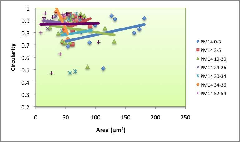
135

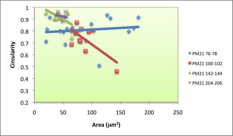
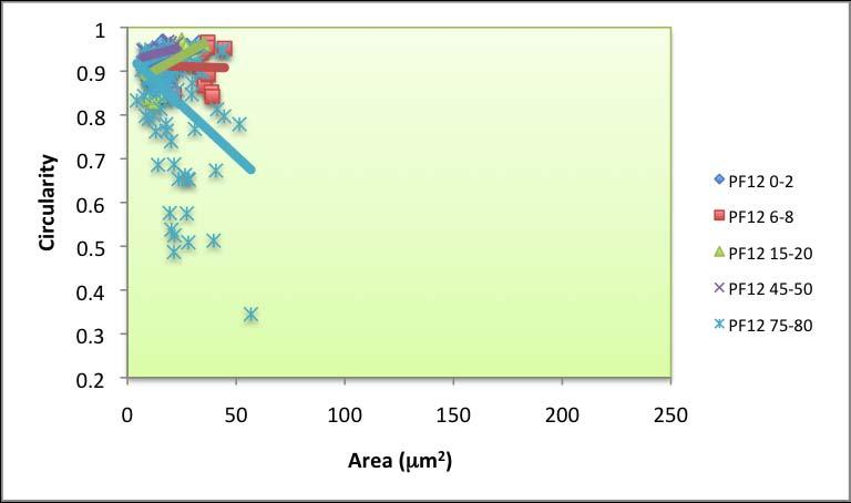
136