Calendar year age estimates of Allerød Younger Dryas sea-level oscillations at Os, western Norway

Transcription

1 Calendar year age estimates of Allerød Younger Dryas sea-level oscillations at Os, western Norway ØYSTEIN S. LOHNE,1,2* STEIN BONDEVIK,3 JAN MANGERUD1,2 and HANS SCHRADER1 1 Department of Earth Science, Alle gaten 41, N-5007 Bergen, Norway 2 The Bjerknes Centre for Climate Research, University of Bergen, Norway 3 Department of Geology, University of Tromsø, Dramsveien 201, N-9037 Tromsø, Norway Abstract: A detailed shoreline displacement curve documents the Younger Dryas transgression in western Norway. The relative sea-level rise was more than 9m in an area which subsequently experienced an emergence of almost 60 m. The sea-level curve is based on the stratigraphy of six isolation basins with bedrock thresholds. Effort has been made to establish an accurate chronology using a calendar year time-scale by 14C wiggle matching and the use of time synchronic markers (the Vedde Ash Bed and the postglacial rise in Betula (birch) pollen). The sea-level curve demonstrates that the Younger Dryas transgression started close to the Allerød Younger Dryas transition and that the high stand was reached only 200 yr before the Younger Dryas Holocene boundary. The sea level remained at the high stand for about 300 yr and 100 yr into Holocene it started to fall rapidly. The peak of the Younger Dryas transgression occurred simultaneously with the maximum extent of the ice-sheet readvance in the area. Our results support earlier geophysical modelling concluding a causal relationship between the Younger Dryas glacier advance and Younger Dryas transgression in western Norway. We argue that the sea-level curve indicates that the Younger Dryas glacial advance started in the late Allerød or close to the Allerød Younger Dryas transition. KEYWORDS: Younger Dryas; sea-level change; isolation basins; western Norway. Introduction Parts of western Norway experienced a rise in relative sea-level of ca. 10m during the Younger Dryas (YD) (Anundsen, 1978, 1985; Krzywinski and Stabell, 1984). The sealevel rise, called the YD transgression (Anundsen, 1978, 1985), reversed the ongoing emergence caused by glacial unloading, and stands in contrast to other areas in Scandinavia, where the YD was characterised by emergence or by a relative sea-level standstill. The YD transgression was restricted to the southwest coast of Norway, a geographical area that also experienced a large (>50 km) glacial YD readvance (Mangerud, 1977, 2004). Geophysical modelling carried out in the 1980s (Fjeldskaar and Kanestrøm, 1980; Anundsen and Fjeldskaar, 1983) suggested that the transgression was the result of three factors: (i) caused by the advancing ice which stopped or reversed the isostatic rebound, (ii) the increased gravitation of the growing ice mass attracted ocean water towards the coastline, and (iii) the rising global eustatic sea-level. According to the modelling and current thinking a combination of these factors led to the YD transgression. If (i) and (ii) are correct, the timing of the transgression should be closely connected to the timing of the glacier readvance. Recently, Bondevik and Mangerud (2002) demonstrated that the YD ice-sheet in western Norway reached its maximum extent only yr before the YD Holocene transition. In this study we focus on the changes in sea-level and try to answer the following questions: 1 When did the YD transgression start and end? 2 What is the relationship between the timing of the YD glacier maximum and the peak of the transgression? In order to answer these two questions we have constructed a detailed sea-level curve with a firm chronology in calendar years. Correlating and dating late-glacial sequences are difficult owing to the so-called radiocarbon plateaux. Two such plateaux, centred at and C yrbp (e.g. Gulliksen et al., 1998; Stuiver et al., 1998) are especially problematic. The plateau lasts for ca. 600 yr (Stuiver et al., 1998) and the plateau lasts for ca. 400 yr (Ammann and Lotter, 1989; Lotter, 1991). To overcome these problems we convert our radiocarbon years to calendar years by using a modified wiggle matching technique to fit series of close radiocarbon dates to the calibration curves. We also take advantage of the Vedde Ash Bed (Mangerud et al., 1984), a synchronous time marker, visible in all our cores. The Vedde Ash has been dated to ca C yr BP (Birks et al., 1996) and ice-core yr BP (Grønvold et al., 1995). In addition, we use the rise of Betula (birch) pollen that we regard as a reliable, local correlation horizon. From other studies the Betula rise is found close to the YD Holocene boundary (Kristiansen et al., 1988; Paus, 1989; Berglund et al., 1994; Bondevik and Mangerud, 2002). In the present study we show that in the Os area, the rise in Betula pollen was slightly delayed compared with the onset of the warming at the YD Holocene boundary, and a calendar year age estimate for the Betula rise is presented. Research strategy and methods Our main strategy to determine past relative sea-level changes has been to use the so-called isolation-basin method (Hafsten, 1960). Lakes and bogs that are located below the marine limit were once part of the sea and thus hold marine sediments in the lower part of their sedimentary sequences. As a result of glacial rebound the basins were subsequently isolated from the sea and turned into lakes. This is recorded as a stratigraphical sequence of marine brackish freshwater sediments in the basin. The transition from marine/brackish to lacustrine sediments, i.e. the stratigraphical level where the lake is isolated from the sea, is called the isolation contact (Hafsten, 1960; Kjemperud, 1986). Where lacustrine sediments are overlain by marine/brackish sediments, the boundary is defined as the ingression contact and it represents the stratigraphical level where the rising sea enters the lake. The isolation and ingression contacts are considered to represent the high tide sealevels, although it is not known whether this reflects daily, monthly or even rarer spring high tides. The present astronomical forced tidal range in the Bergen area is 170cm (Tidevannstabeller, 1998). We emphasise that with the isolation basin method, the relative sea-level is measured as the elevation of the outlet threshold, not the (lower) elevation of the isolation and ingression contacts in the lake sediments. Therefore, only basins with an outlet across a bedrock threshold are used, so that negligible erosion is expected after the lake was isolated from the sea. The thresholds were preferably levelled to survey control points with datum level (NN1954) approximately at mean sea-level (Tidevannstabeller, 1998). For one remote basin, however, we used the upper limit of the brown algae Fucus vesiculosus, which is found to be slightly ( m) above mean sea-level (Rekstad, 1908; Møller and Sollid, 1972). Cross-sections of each basin were cored with a Russian peat corer and the cores were described in the field. Based on this mapping we selected sites that we cored with a piston corer, using PVC tubes with a diameter of 110 mm. In the laboratory, the cores were splitted lengthways, described in detail and subsampled. The sedimentary sequences were classified in informal lithostratigraphical units. Some intervals of the cores were X-radiographed to identify sedimentary structures, molluscs and clasts. Samples for loss-on-ignition analysis were dried for 24 h at 105 C and ignited at 550 C for 1 h. Weight of loss was calculated as percentage of the dried sample weight. The Vedde Ash Bed was visible to the naked eye in all of the basins studied. Nevertheless, in one basin the ash particles >63 m were identified and counted under a stereomicroscope. Two types of ash particles were found, corresponding in colour and morphology to the rhyolitic and the basaltic fraction of the Vedde Ash Bed (Mangerud et

2 al., 1984). Radiocarbon dates were preferably obtained by AMS on terrestrial plant macrofossils in order to avoid problems with lake hardwater (Barnekow et al., 1998) and marine reservoir effects (Mangerud and Gulliksen, 1975). Some dates, however, were obtained from marine molluscs and bulk gyttja samples. The sediments were analysed for diatoms at critical levels, and the isolation and ingression contacts were identified. The diatom analysis has been somewhat simplified compared with earlier similar studies (e.g. Lie et al., 1983; Krzywinski and Stabell, 1984; Corner and Haugane, 1993). The samples are generally rich in diatoms and the analysis was performed on smear slides, where a small portion of bulk sediment was mounted on the slide using Mountex (RI-1.67). The advantage of this technique is the minimised loss of small diatoms during preparation, as well as saving time. Flocculation of diatoms and sediment particles sometimes occurred, however, especially in organic-rich sediments, causing a more problematic identification and counting of the valves. In one of the basins (Langevatnet) we also used a simplified counting technique where the most common species of the marine and lacustrine environment were found by traditional counting of all species. These countings were performed at 15 levels representing all the sedimentary units. The 32 most common species were found and counted at additional 20 levels throughout the analysed part of the core. This way of analysing diatoms is found to be of sufficient quality for detecting such large water chemistry changes as during an isolation of a lake (Corner and Haugane, 1993). In the other basins (Grindavoll, Særvikmyra and Lysevågvatnet) the traditional method of counting all species was undertaken. Methods for convert the 14C chronology to calendar year time-scale are presented in a section below. The calendar ages of the chronozone boundaries follows the calibration data sets (see chronology section), where the YD Holocene boundary is at cal. yr BP (Spurk et al., 1998) and the Allerød YD transition is at cal. yr BP (Hughen et al., 2000). The basins studied The basins studied are presented in order of their elevation from highest to lowest (Table 1). The conversion to the calendar year time-scale is presented collectively for all the basins in a separate section. Grindavoll (58.0m a.s.l.) Lithostratigraphy At Grindavoll (Fig. 1) a cultivated mire covers a palaeolake basin ca. 150m long and a 60m wide. Early in the twentieth century the outlet sill was lowered by about 1.4m in order to drain the mire. We reconstructed the original bedrock threshold to an elevation of m a.s.l. The basin has two subbasins that are separated by a bedrock sill with a former water depth of only about 1.3m (Fig. 2). A creek draining most of the catchment area enters the northern basin (Table 1), whereas the outlet is from the southern basin. This setting is reflected in the sedimentation pattern where the northern basin has more sediments brought in by the creek (especially the Vedde Ash), whereas the southern basin shows a more distinct brackish signal during a period when sea-water entered the basin. For the latter reason, the diatom investigations were performed on a 110mm piston core from the southern basin (505-16; Fig. 2). A summary of descriptions and analyses is presented in Fig. 3. The sediment sequence is divided into five units (Fig. 3). The basal unit is bluish grey silt with sand layers/lamina. Diatoms are nearly absent, and even though almost all species identified are of lacustrine habitat it is impossible to rule out a marine environment. The unit is interpreted as a probably lacustrine or possibly marine, proglacial deposit. At 565 cm depth a grey 2-mm-thick lamina of Vedde Ash particles occurs. The bright colour is probably due to dominance of the colourless rhyolitic particles (Fig. 3). In the northern basin the ash layer varies from 7 to 15 cm, increasing in thickness towards the mouth of the inlet creek (Fig. 2), and it consists of alternating black and grey laminae. Most of the ash particles were brought to the lake by the creek, and sorted in the lake according to particle size, shape and density. In the southern basin the ash bed is primarily composed of low-density rhyolitic particles, more easily transported across the internal sill, and giving the light grey appearance. The gyttja-silt unit between 561 and 551cm differs from the underlying unit by higher silt content, a greyish colour, drop in the LOI curve, and by its alternating zones with colourful, fine laminations. Diatoms show a pronounced brackish signal with up to 50% of salt-demanding species in the middle of the unit. This occurrence decreases towards the top of the unit. A short pollen diagram (six samples) reveals the post-glacial Betula rise at 554 cm depth (Appendix 1). The overlying unit consists of brownish gyttja, with LOI values of about 40% indicating almost pure organic sediments, typical for Holocene deposits in coastal lakes in western Norway.

3 Figure 1The area studied is located in Os about 25 km south of Bergen on the western coast of Norway. (A) Key map of southern Norway, with YD icemargin(dot-dashlines) (Mangerud,2004).(B)TheYDisobases(dashedlines)are constructed from marine limit terraces(*) deposited in front of the YD ice-marginal Herdla Moraines (dot-dash lines) (Aarseth and Mangerud, 1974). (C) Location of the sites investigated, with the elevation (m a.s.l.)of marine limit terraces (numbers in italic) and the baseline for the shoreline displacement curve (58 m Younger Dryas isobase). Dark grey fill indicates areas above the marine limit, grey indicates present land below the marine limit and light grey shows areas within the former YD ice-sheet. Dot-dash line indicates ice-sheet margin from Aarseth and Mangerud (1974); short-dash line indicates ice-sheet margin based on other criteria Figure 2 Cross-section of the basin at Grindavoll; cores are shown as vertical lines. Core is shown in Fig. 3. The outlet threshold is at the southwest end. Note the differences in thickness of Late Weichselian sediments and especially thevedde Ash Bed(black) between the two sub-basins. Legend for sediment types is given in Fig. 3 Sea-level changes at Grindavoll Finely laminated sediments, as found between 561 and 551cm in the Grindavoll record, are well known to occur during the brackish phase of the isolation of a basin from the sea (Kaland, 1984; Svendsen and Mangerud, 1987). At Grindavoll, the brackish water phase is also demonstrated by diatoms, indicating that marine water entered the lake late in the YD (Fig. 3). The low content (<50%) of the brackish/marine diatoms indicates that the sea-water only occasionally, at very high tides, flowed into the basin. The sediments below and above the laminations contain solely lacustrine diatoms. Thus, the Grindavoll site records the absolute maximum level of the transgression late in the YD, at an elevation of 58.0+/-0.5m a.s.l. This is slightly above the elevations of the nearby marine terraces at 57m a.s.l. of YD age (Aarseth and Mangerud, 1974) (Fig. 1A). The base and top of this marine-influenced unit are hereafter referred to as ingression and isolation contacts even though the Grindavoll Basin never really became part of the sea. The pre-yd record at the Grindavoll site indicates a sea-level below the threshold. Nevertheless, minor uncertainties exist for the early deglaciation, where diatoms are nearly absent, leaving the question about high sea-level during the deglaciation unsolved. Langevatnet (50.3 m a.s.l.) Lithostratigraphy

4 Langevatnet ( vatnet =lake) is a narrow lake about 800m long (Fig. 4). The outlet is across a bedrock sill at the southwest end, levelled to 50.3m a.s.l. (Table 1). Seven locations were cored (Fig. 4) and the lithology was easily correlated between them. Core , obtained from the deepest part, was used for the analysis and is further described in Fig. 5 and in Appendices 2 and 3. The basal unit is a bluish silt unit with layers of sand (Fig. 5), very low LOI values and nearly devoid of diatoms, probably deposited during the deglaciation of the area. The overlying marine unit ( cm) indicates that the basin was below sea-level during deglaciation, and that the basal unit thus has a glaciomarine origin, even though a few freshwater diatoms were identified. These are probably related to inflow of fresh meltwater into the basin. The date of C yr BP from a Mytilus edulis shell from the overlying unit (Table 2) provides a minimum age of the deglaciation. The densely laminated gyttja silt ( cm depth) represents the first isolation from the sea (Fig. 5). The overlying lacustrine unit consists mainly of brownish, partly laminated silt gyttja with scattered plant remains, which have been 14C dated at four levels (Fig. 5). According to the dates this unit extends through the Allerød Younger Dryas transition, but the boundary is not visually detectable. The following units ( cm) have marine diatom floras, showing that the basin was again submerged. Owing to lack of terrestrial plant remains near the ingression contact, there is no 14C date for this event. However, the Vedde Ash Bed appears as a visible black layer 3 cm thick, 8 cm above the ingression contact. Figure 3 The stratigraphy of Grindavoll (core ). Most of the plant remains are stems of mosses and leaves of Salix herbacea. Detailed diatom and pollen diagrams fromgrindavoll are shown in Appendix 1. Diatom salinity groups: P, polyhalobous; M, mesohalobous; O-H, oligohalobous halophilous; O-I, oligohalobous indifferent; H, halophobous Figure 4(A) Map of Langevatnet (note the oblique arrow towards north). Cores marked in Roman numbers are Russian peat cores, whereas arabic numbers mark the 110 mm piston cores (01 = , 02 = , 03 =505-03). Contour interval of 10 m. Three minor creeks and the outlet of the lake are marked by arrows in flow direction. (B) Longitudinal profile. Vertical scale is in metres below the lake surface (50.3 m a.s.l.) and horizontal scale in metres from the outlet sill The Vedde Ash bed is found in a gyttja-silt unit with scattered cobbles and pebbles, probably produced by active frost weathering on the YD shoreline and dropped from seaice (Blikra and Longva, 1995; Bondevik et al., 1999; Bondevik and Mangerud, 2002). The existence of sea-ice is also indicated by the high occurrence of the sea-ice diatom Fragilariopsis cylindrus (Gersonde and Zielinski, 2000) throughout the unit. A gradual increase of plant fragments and a disappearance of dropstones mark the base of the overlying unit, which is laminated in the upper part. Even though no dropstones occur in this unit, the presence of the sea-ice indicator F. cylindrus through most of the unit

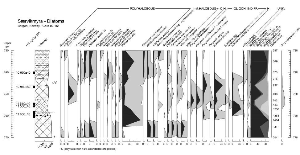
5 suggests a cold environment and sea-ice cover. In the uppermost part of the unit at 2147 cm depth, the diatom flora is replaced by more temperate species, dominated by Thalassionema nitzschioides (de Wolf, 1982). This indicates a shift to warmer conditions reflecting the YD Holocene boundary, and is further supported by a short pollen diagram (Appendix 3), revealing the classic early post-glacial Betula rise 2 cm further up, marked at 2145cm depth in Fig. 5. A 2-cm-thick densely laminated silt gyttja shows the final isolation of Langevatnet (Fig. 5). Through this unit, the LOI curve increases from 5% to more then 20%. The uppermost dark brown gyttja is the lower part of the 450 cm post-glacial organic sediments not shown in Fig. 5. Seven dates were obtained from this unit ranging from to C yrbp (Fig. 5 and Table 2). Sea-level changes at Langevatnet After a period of marine conditions following the deglaciation, the relative sea-level fell and Langevatnet became a freshwater lake at C yr BP. The lacustrine environment prevailed through Allerød (AL), before the sea-level again rose above the basin early in the YD, between C yr BP and the Vedde Ash Bed (ca C yr BP). Marine conditions prevailed beyond the YD Holocene boundary, as indicated by both pollen and diatoms. Langevatnet was finally isolated during the early Holocene, dated to C yr BP. Særvikmyra (44m a.s.l.) Lithostratigraphy Særvikmyra ( myr =bog) (Fig. 1 and Table 1) is a well-defined basin, surrounded by hills up to 100m high. The outlet is a narrow bedrock threshold. Presently the basin is a bog, partly covered with pine trees. Særvikmyra is located in a nature reserve remote from any road, and for this reason easy transportable equipment was used. The cores analysed were obtained by a 110mm Russian peat corer, and the basin elevation was levelled from the present shoreline (using the upper limit of Fucus vesiculosus). Above the lowermost bluish grey laminated deglaciation sequence (not shown in Fig. 6), there are several units of silty sediments, dated between and C yr BP (Fig. 6). The diatoms and the frequent shell fragments demonstrate a marine origin for the main part these sediments. The exception is an 18-cm-thick interval consisting of two layers of brownish silty gyttja separated by a layer of sandy silt. The two brownish units have a mixed diatom assemblage with both marine and up to 80% lacustrine diatoms (Fig. 6), whereas the sandy silt between is dominated by marine diatoms. This 18 cm interval has been dated to C yr BP. The Vedde Ash Bed is seen as a 1.5-cm-thick layer at 726cm depth. A sharp boundary, 3 cm above the ash bed, forms the base of about 70 cm of bluish-grey laminated silt; a typical glaciomarine sediment. We conclude that it corresponds to the YD glacier maximum located less than 2 km east of the site (Fig. 1). The stratigraphy supports the conclusion of Bondevik and Mangerud (2002) that the YD glacial maximum was reached after the Vedde Ash fall. This unit is overlain by 640cm of Holocene lacustrine gyttja and peat. Sea-level changes at Særvikmyra The mixed diatom flora of the brownish layers at Særvikmyra is dominated by the marine Paralia sulcata and the freshwater Fragilaria spp. These are all euryhaline (tolerating large salinity variations) and are typically found near isolation and ingression contacts (Stabell, 1985; Zong, 1997) where the water salinities are highly variable. This implies a sea-level close to the basin threshold for the period between C yr BP, but the presence of marine diatoms shows that Særvikmyra did not became a true lake in the Allerød. Særvikmyra precisely records the regression minimum in the mid- to late Allerød. The sandy silt layer between the brownish/brackish layers may represent a minor rise of the sea-level during the sea-level lowstand. At about C yr BP the basin was finally isolated from the sea, and was a lake until it was filled up and became a bog. Lysevågvatnet (20.7m a.s.l.) Lithostratigraphy Lysevågvatnet (Fig. 1) is a rectangular lake (150x80 m), with a flat bottom and a water depth of about 9 m. The lake has a bedrock sill towards the northwest with a present elevation of 20.7m a.s.l. The northernmost (505-12) of three 110-mm cores was used for the analysis. The deposit can be divided into three units (Fig. 7). The lower marine, olive-grey silt gyttja unit contains frequent mollusc fragments. Above this, a 1-cm distinct bed of greenish black gyttja, restricted by sharp boundaries, forms a unit with typical brackish sedimentary facies. It lacks minerogenic particles; has a fatty appearance, is nearly impossible to disperse in water, and it reveals a clear thin layering when mechanically broken. The diatom flora is also dominated by brackish species. The uppermost unit is lacustrine gyttja.we found no indications of lacustrine sedimentation in the deeper part of the stratigraphy of Lysevågvatnet.

6 Figure 5 The stratigraphy of Langevatnet (core ). The lowermost date is obtained from a neighbouring core ( see Fig. 4) and correlated by lithology to core The diatoms are grouped in one marine group including poly- and mesohalobous species, and one lacustrine group including oligohalobous indifferent and halophobous species. Detailed diatom and pollen diagrams from Langevatnet are shown in Appendix 2 and 3 Table 2 Radiocarbon dates of terrestrial and marine material from Langevatnet, Grindavoll, Stølsmyra and Lysevågvatnet. Numbers prefixed by TUa, Beta and Poz are dated by accelerator mass spectrometry (AMS) analysis at the Svedberg Laboratory, Uppsala University (Sweden), Beta Analytic Inc. (USA) and Poznan Radiocarbon Laboratory (Poland) respectively. Conventionally dated samples (T prefix) were performed at the Radiological Dating Laboratory in Trondheim (Norway) Figure 6 The stratigraphy of Særvikmyra (core /152). Diatom analysis is conducted for the interval cm; other diatom information is based on only a brief microscopic check of slides. Diatom salinity groups: P, polyhalobous; M, mesohalobous; O-H, oligohalobous halophilous; O-I, oligohalobous indifferent; H, halophobous. See Table 2 for details about dates. Detailed diatom diagram from Særvikmyra is shown in Appendix 4

7 Figure 7 The stratigraphy of Lysevågvatnet (core ). The Vedde Ash Bed is present in the core at a depth of 1509 cm, not shown here. Detailed diatom diagram from Lysevågvatnet is shown in Appendix 5. Diatom salinity groups: P, polyhalobous; M, mesohalobous; O-H, oligohalobous halophilous; O-I, oligohalobous indifferent; H, halophobous Sea-level changes at Lysevågvatnet The deposits in Lysevågvatnet record a falling relative sealevel, which at C yr BP was at 20.7m a.s.l. The isolation shows a typical diatom and sedimentological succession for basins isolated early in the Holocene when the sea-level dropped rapidly (Kaland, 1984). Chronology and age models In order to establish the sea-level chronology in calendar years, we estimate the ages using a wiggle-matching technique modified after Pearson (1986) or standard CALIB v4.3 calibration (Stuiver and Reimer, 1993; Stuiver et al., 1998). The most precise chronology was established at the key locality Langevatnet. The wiggle matching technique was used originally on sequences with an independent floating annual time-scale (e.g. annual laminated sediments). For records without an independent floating time-scale, such as the non-varved lake sediments presented here, sedimentation rates have to be estimated (Gulliksen et al., 1998). In this paper we assume constant sediment accumulation between dates within the same sedimentary unit. The pattern of each series of dates is fitted to a calibration curve, allowing both the position and the numbers of years between the dates to vary. This is done by calculating the sum of differences (SOD) for every position of the data set (1-yr steps) with respect to a wide range of sediment accumulation rates (SAR) (steps of 0.1 yrcm ¹). Smaller SOD values reflect better agreement with the calibration curve. The result is presented as a plot of the absolute lowest SOD value obtained, at the specific calendar year. A step-by-step description of the procedure is presented in Appendix 6. The calibration curve is well established back to about cal. yr BP, where the curve is based on tree-ring chronologies (Stuiver et al., 1998). Prior to cal. yr BP, there are still no absolute dated chronologies available (van der Plicht, 2002; Litt et al., 2003). We have used the high-resolution Cariaco series (Hughen et al., 2000) for events older than cal. yr BP, even though it seems evident that the included constant marine reservoir correction of 420 yr is an underestimation for some intervals (Litt et al., 2003).

8 Langevatnet Two series of 14C dates from Langevatnet are wiggle matched: (1) the early Holocene lacustrine sediments estimating the age of the final isolation contact (Fig. 5), and (2) the Allerød and YD lacustrine sediments estimating the age of the first isolation contact and the ingression contact. 1 The match of the seven dates in the early Holocene series (the outlier TUa-2178 is omitted) revealed best-fit SAR values around yr cm ¹. The SOD plot shows a distinct minimum for a position of the isolation between and cal. yr BP, with the best fit at cal. yr BP, obtained with a SAR of 34.4 yr cm ¹ (Fig. 8). 2 The estimate of the older isolation contact shows a fairly well-constrained minimum between and cal. yr BP, with the best fit at cal. yr BP, obtained for a SAR value of 36.5 yr cm ¹ (Fig. 8 and Table 3). The SOD curve for the ingression has a wider minimum, however, as a result of scarcity of dates in the upper part of the series. Low values were obtained for the entire interval cal. yr BP, with lowest SOD for cal. yr BP for the ingression. Extending the age back to cal. yr BP, however, would lead to an unrealistic increase of the SAR for the overlying marine sediment between the ingression and the Vedde Ash (up to 93 yr cm ¹). In order to test the result, a new match was performed with the series tied to the Vedde Ash at cal. yr BP (Grönvold et al., 1995). Similar results were obtained for both the SAR and the position of the series, supporting the original match at cal. yr BP. An age model for Langevatnet is constructed from the results of the wiggle matching, the YD Holocene transition of cal. yr BP (Spurk et al., 1998; Stuiver et al., 1998) and the Vedde Ash at cal. yr BP (Fig. 9). The YD Holocene transition is identified as a decrease of the sea-ice diatom Fragilariopsis cylindrus and an incipient appearance of Thalassionema nitzschioides at 2147 cm depth. This latter species is associated with warm and highly saline water typical of the Norwegian Atlantic current in the northern Atlantic area (Koc Karpuz and Schrader, 1990; Jiang, 1996). A similar diatom transition at this boundary is also reported in the ocean off the Norwegian northwest coast (Koc Karpuz and Jansen, 1992) and in the Skagerrak Kattegat area (Jiang et al., 1997). Diatoms respond quickly to environmental changes (Dixit et al., 1992) and are probably a relatively precise proxy of the climatic change at the YD Holocene transition. The resulting age model estimates an age of the Betula rise some yr after the YD Holocene transition, ca cal. yr BP. Because of the difficulties with the 14C calibration in the time interval in the lower part of the core, the single date C yr BP (Fig. 5) is not sufficient to estimate an independent SAR for the oldest marine unit. The age model (Fig. 9) is constructed with a sediment accumulation rate from the similar sediments of the early Holocene marine unit, giving an age of ca cal. yr BP for the deglaciation in Langevatnet. Særvikmyra The series of five dates from the regression minimum sediments in the Allerød was wiggle matched to the Cariaco basin data (Fig. 10). For the isolation low SOD values were obtained in the interval cal. yr BP, and for the succeeding ingression in the interval of cal. yr BP. The SAR value of 35.5 yrcm 1 resulted in the best fit, with ages for the isolation and the ingression respectively of and cal. yr BP (Fig. 10 and Table 3). The sea-level rise occurred according to the dating at or close to the Allerød YD transition. Floating tree-ring chronologies, however, indicate that minor plateaux occur prior to the YD, which are not seen in the Cariaco Basin calibration data set (Litt et al., 2003). The latter is therefore probably inaccurate for this period. In order to identify the Allerød YD transition at Særvikmyra we conducted a restricted pollen analysis (not shown here), which showed a climatic reversal at about 740 cm depth. This may be the Allerød YD transition, but pollen sums were low (40 100) so no firm conclusions can be drawn. It indicates, however that the ingression (742.5 cm depth) at Særvikmyra occurred slightly before the onset of the YD. Grindavoll The isolation at Grindavoll occurred after the Betula rise, dated to cal. yr BP in Langevatnet, and because it is at a higher elevation, before the isolation in Langevatnet. Thus the isolation at Grindavoll is bracketed between and cal. yr BP. However, as the isolation is located 3 cm above the Betula rise (Fig. 3), and that more than 3m lowering of the sea-level took place between the isolation of Grindavoll and Langevatnet, an estimate of about cal. yr BP for the isolation of Grindavoll seems reasonable. The ingression at Grindavoll occurred between the Vedde Ash Bed (ca cal. yr BP) and the Betula rise at ca cal. yr BP (Fig. 3). A simple linear interpolation between these two levels results in an age of cal. yr BP, but does not incorporate a probable increased sediment accumulation after the ingression. A more likely estimate is calculated by extrapolating downwards the sediment accumulation rate between the isolation contact and the Betula rise, which results in an estimated age of about cal. yr BP for the ingression contact at Grindavoll (Table 3).

9 Figure 8 The 14C dates from the lacustrine unit younger than C yr BP were wiggle matched to the INTCAL98 calibration curve (Stuiver et tal., 1998). The best fit, i.e. the lowest sum of differences (SOD), was obtained with a constant sedimentation rate of 34.4 yr cm 1 and with an age of the isolation contact (2138 cm) of cal. yr BP. The outlier date TUa-2178 (Table 1) was not used. The 14C dates below the Vedde Ash Bed were wiggle matched to the Cariaco basin data (Hughen et tal., 2000). Best fit was obtained with a constant sedimentation rate of 36.5 yr cm 1 and a location of the isolation contact (2256 cm) at cal. yr BP and the ingression contact (2205 cm) at cal. yr BP. Radiocarbon dates are plotted with +/-2σ according to the best fit from the wiggle matching. Shaded grey areas show age interval with SOD < <15, which are regarded as a good fit (Table 3). Non-linear depth scale is according to the age model shown in Fig. 9. For further explanation see text

10 The sea-level curve from Os The thresholds of the basins are not located on the same isobase and in order to construct a sea-level curve from one single site we had to correct their elevations for the tilted isostatic uplift. All the basins are located relatively close to the baseline and minor uncertainties in the tilt corrections are insignificant for the curve. We adjusted all elevations to the 58-m isobase that runs through the terrace at Ulven (Fig. 1C). The five uppermost basins, isolated close to the YD Holocene boundary, were adjusted using a gradient of 1.3m km ¹ (Table 1). This estimate is calculated from several YD terraces in the Os area (Anundsen, 1985) and strictly valid only for the YD. We also used this number for pre-yd gradients, and consider this as a minor error for the sea-level curve. However, the pre-yd gradients will be tested in the further progress of this project. The Holocene shoreline gradients are fairly well known (Hamborg, 1983; Kaland, 1984), and the elevation of Lysevågvatnet is corrected according to the C yr BP shoreline with a tilt of 0.5 m km ¹ (Table 1). The exact elevation of the sea-level following the deglaciation is unknown. There are no marine terraces above the YD terraces in this area. Langevatnet is the highest basin that shows unquestionable marine deposits after the deglaciation. We conclude that the relative sea-level during the deglaciation was between the elevation of Langevatnet and the YD level, i.e. between 55 and 58m a.s.l. (Fig. 11A). The sea-level reached a minimum level of 49.2m a.s.l. defined by brackish sediments in Særvikmyra estimated to cal. yr BP (Table 3). A minor fluctuation of the sealevel occurred before the sea-level again rose at about cal. yr BP. The level of the regression minimum is supported by the Kloppamyra and Stølsmyra basins described by Bondevik and Mangerud (2002). At approximately cal. yr BP, slightly before the Vedde Ash fall (Figs 5 and 11A), the sea-level had risen to Langevatnet again, and continued to rise to the transgression maximum at about 58.5m a.s.l., as well-defined at Grindavoll. The Os sea-level curve defines precisely both the Allerød regression minimum and the YD transgression maximum, giving an amplitude of the transgression of about 9m. According to the Grindavoll basin the maximum of the transgression culminated at about cal. yr BP (Fig. 11A). Subsequently the sea-level was relatively stable for 300 yr with extreme high tides just above the threshold of the Grindavoll basin. During this time span the marine limit terraces were formed. After the Betula rise, the marine influence at Grindavoll ceased, and the major post-glacial regression started. As discussed above, we estimate the age of the start of this major regression at about cal. yr BP (Table 3). Hence, the regression started soon but distinctly after the YD Holocene boundary, which is demonstrated by both pollen stratigraphy and dates. After the isolation of Grindavoll the relative sea-level fell rapidly, and Langevatnet (54.7m a.s.l.) was isolated at cal. yr BP, and Lysevågvatnet (22.3m a.s.l.) was isolated at about cal. yr BP (Table 3). This results in an average rate of regression of about 5 cm yr ¹ from the marine limit to 22.2m a.s.l.

11 Figure 11 (A) The relative sea-level curve for the Os area based on the calendar year ages of isolation and ingression contacts in the studied basins (Table 3). The stratigraphy in each basin is plotted as a full line for periods with marine sedimentation and a dotted line for periods of lacustrine sedimentation. The Vedde Ash (V) and the pollen-stratigraphical Betula rise (B) are plotted as dashed vertical lines. The timing of the YD glacier maximum in this area (Bondevik and Mangerud, 2002) defined by glaciomarine sediments in basins, is shown as a shaded bar. The course of the global glacio-eustatic sea-levels (Fairbanks, 1989; Lambeck et al., 2002) are indicated above the sea-level curve. Sea-level data from Kloppamyra and Stølsmyra (Fig. 1) are also included (Bondevik and Mangerud, 2002). (B) Time distance diagram of ice-front variations in the Bergen district plotted on a similar and vertically aligned time-scale, modified from Mangerud (1977). An alternative course of the YD glacier advance, outlined from the sealevel curve from Os (above), is included Discussion The Younger Dryas transgression According to the Særvikmyra record the YD transgression started at or probably slightly before the Allerød YD transition (Fig. 11A). This is somewhat later than shown by former published sea-level curves from western Norway. The curves from Sotra (Fig. 1B) and Boknafjorden (Fig. 1A) indicate that the transgression began in the early mid- Allerød (Anundsen, 1985). At Sotra the ingression contacts from several basins are dated C yr BP (Krzywinski and Stabell, 1984), but as these are bulk gyttja dates performed on 5-cm-thick sediment slices the divergency to the Os curve may be assigned to inaccurate dates. We have shown that the YD transgression in the Os area culminated very late in the YD. This is later than interpreted for the Sotra curve and other sea-level curves in western Norway. We consider this also to be related to the accuracy of the 14C dates, but partly also to the elevations of the investigated basins, and the original estimate of the Vedde Ash Bed (Mangerud et al., 1984; Birks et al., 1996), which was 300 yr too old. Another striking effect of the improved chronology is the timing of the major post-glacial regression. The onset of the regression was earlier dated to the later part of the YD chronozone (Krzywinski and Stabell, 1984; Anundsen, 1985). However, all of the dates used fall within the C yr BP plateau. We have now demonstrated that the start of the regression post-dates the Betula rise and that the Betula rise post-dates the warming at the YD Holocene boundary. At Sotra only 20km from Os, the emergence also starts after the first rise of Betula, but this rise was originally placed within the YD chronozone (Krzywinski and Stabell, 1984; Anundsen, 1985). This first Betula increase, however, is accompanied with rises in both Empetrum and Juniperus and a decrease in Artemisia, which is typical for the YD Holocene boundary (Kristiansen et al., 1988). We therefore conclude that the major regression commenced after the YD/Holocene boundary also on Sotra. Similar reinterpretations are also possible for the sealevel curves around Boknafjorden (Fig. 1) (Thomsen, 1982, 1989; Anundsen, 1985). Sea-level change and ice-sheet fluctuations

12 A striking synchroneity between the maximum position of the YD ice-sheet at cal. yr BP (Bondevik and Mangerud, 2002) and the transgression maximum at cal. yr BP, occurs in the Os area. The onset of the regression was slightly delayed, however, as it started ca yr after the Betula rise, whereas the ice started to retreat at the time of the Betula rise. Geophysical modelling suggests that the YD transgression was a result of increased gravitational attraction of the advancing ice-sheet, in combination with halted isostatic uplift as the ice load increased and a rising eustatic sea-level (Fjeldskaar and Kanestrøm, 1980; Anundsen and Fjeldskaar, 1983). Another argument is that the transgression occurred only along the southwest coast of Norway, where the glacial readvance was largest (Anundsen, 1985; Mangerud, 2004). In Sunnmøre (Fig. 1A, where the glacier fluctuations were minor, there was a sea-level stillstand during the YD (Svendsen and Mangerud, 1987). The fact that this major transgression was restricted to a part of western Norway, excludes global eustatic sea-level rise as the only or dominating cause for the transgression. In addition, the ages of the meltwater pulses, MWP-1A and MWP-1B (Fairbanks, 1989), are not consistent with the timing of the YD transgression (Fig. 11). The strong synchroneity between the maximum position of the YD icesheet and the transgression maximum shown in this study, further supports the link between ice-sheet advance and the sea-level response. If we accept these causative relations, the sea-level curve at Os indicates a glacier retreat from to about cal. yr BP. This retreat is succeeded by a stabilisation of the ice-sheet where regional sea-level components more or less equal the eustatic sea-level rise. The stable phase prevailed for about 500 yr until the sea-level started to rise in the late Allerød or at the Allerød YD transition, as a result of the renewed glacier build-up. This indicates that the glacier build-up possibly started prior to the climatic reversal at the Allerød YD boundary. The fast sea-level rise during the first part of the YD may indicate an earlier and faster readvance (Fig. 11) than postulated by Mangerud (1977, 2000, 2004). Other studies from Norway also suggest that the YD glacier expansion started late in the Allerød (Bergstrøm, 1999; Vorren and Plassen, 2002). The YD climates in western Norway were cold but also dry (Dahl and Nesje, 1992; Birks et al., 1994). The low precipitation would indicate slow accumulation and does not favour a massive ice-sheet reactivation. Nevertheless glacier expansion during the YD is recorded by cirque glaciers (Larsen et al., 1984), local ice domes (Sønstegaard et al., 1999) and the inland ice-sheet (Mangerud, 1977, 2000, 2004; Bondevik and Mangerud, 2002). In the Allerød the climate was milder than during the YD, but with relatively high precipitation (Birks et al., 1994). Many cirque glaciers, even at low elevations, survived throughout the Allerød (Larsen et al., 1998). Probably only minor climatic changes would initiate glacier expansion. A cooling about 100 cal. yr before the YD is registered by aquatic faunal remains in Kråkenes Lake (Fig. 1A) (Birks et al., 2000). Together with sustained high precipitation this may have initiated the glacier advance in the late Allerød, as suggested above. Younger Dryas shoreline features There were contrasting rates of shore erosion in bedrock along the northern European shores during the YD. Distinct rock platforms are found along the YD shorelines both in northern Norway (e.g. Marthinussen, 1960; Rasmussen, 1981) and in Scotland (e.g. Sissons, 1974; Dawson et al., 1999). Cosmogenic exposure dating of the platform in Scotland also supports the YD age (Stone et al., 1996). However, along the southwest coast of Norway no distinct erosional features in bedrock are observed along the YD shoreline. The shoreline only appears as ice-marginal deltas deposited in front of the YD ice-sheet (Aarseth and Mangerud, 1974). The difference in shoreline development may be explained partly by differences in sea-level history. As southwest Norway experienced a rising relative sea-level during most of the YD (Fig. 11), the cold climate shore erosion was not concentrated at one level over a long period, in contrast to what is postulated in northern Norway and Scotland. However, this cannot be the complete explanation. At Sunnmøre (Fig. 1A), welldocumented sea-level histories show a minor fall or standstill during the YD (Svendsen and Mangerud, 1987). Nevertheless no extensive YD shoreline was developed in bedrock, although, frost-shattered stones are common in YD coastal deposits at Sunnmøre (Blikra and Longva, 1995). Similar differences in the processes of cold climate shore erosion are also described and discussed from parts of Scotland (Dawson, 1988, 1989; Gray, 1989). At present the causes for the differences are not fully understood. Conclusions 1 The Younger Dryas transgression started in the late Allerød or at the Allerød Younger Dryas transition and culminated after the deposition in the Vedde Ash Bed in the very late part of the Younger Dryas. The high relative sea-level lasted for about yr, and the major post-glacial regression started approximately 100 yr after the end of the Younger Dryas. 2 In the Os area the Younger Dryas maximum sea-level occurred simultaneously with the maximum extension of the Younger Dryas ice-sheet. The strong synchroneity supports the hypothesis that the cause for the transgression was the large Younger Dryas glacial readvance in this part of Norway. 3 The onset of the fast early Holocene regression was delayed about yr compared with the start of the ice-margin retreat. 4 The sea-level history indicates that the major ice-sheet advance started in the latest part of the Allerød or at the Allerød Younger Dryas transition. Acknowledgements Hilary Birks kindly assisted in the identification of plant macrofossils for dating. Oddmund Soldal at Interconsult Group ASA performed the Georadar measurements of the basin at Grindavoll. Anne Bjune and Victoria Razina conducted the pollen analysis. Herbjørn Heggen, Jorid Lavik, Anne Birgitte Roe and Knut I. Lohne assisted in the fieldwork, Stig Monsen conducted the LOI analysis. Steinar Gulliksen at the Radiological Laboratory in Trondheim was responsible for most of the radiocarbon dating. The journal reviewers, Alastair Dawson and Roland Gehrels, are thanked for constructive remarks, and the latter also for improving the language. We are grateful for the contributions from all these persons, and offer them our sincere thanks. Appendix 1

13 Appendix 2

14 Appendix 3 Appendix 4 Appendix 5

15 Appendix 6 Step-by-step description of the wiggle matching procedure used for estimating calendar year ages. The calculations were performed in a Microsoft Excel Spreadsheet with programming in Visual Basic. 1 The calibration data set (INTCAL98 and Cariaco) was linearly interpolated, in order to assign a 14C age for every single calendar year. 2 The calendar age interval (start- and stop position) for the runs was selected in respect to the stratigraphical level that was to be age-estimated (e.g. isolation contact), hereafter called event. It is important that this interval covers a wide range (>the CALIB calibrated 2 intervals of a 14C date of the event). For the first run the calendar age position (P) of the event was set to the selected start position. 3 The interval of SAR (sediment accumulation rates) for the runs was selected (typically yr cm ¹), together with the step of SAR between each calculation (typically 0.1 yr cm ¹). 4 The calendar age for each of the other 14C dates in the sequence was calculated using the P, the SAR and the depth difference to P. The SOD (sum of differences) was then calculated according to the formula where n is the number of dates, 14Csample,i is the 14C age of the sample i, 14Ccal.curve,i is the 14C age in the calibration data set to the calendar year position of sample i, and is the standard deviation of sample i. 5 The SAR value was increased by one-step and the procedure was repeated from step 4 until the entire SAR interval was tested for the specific position P. 6 The absolute minimum SOD value for the specific P was saved. The P was then moved 1 year, and the procedure was repeated from step 4 until the entire position interval (start to stop position) was tested in respect of all the SAR. 7 The result was plotted as a curve showing the absolute minimum SOD value obtained at each specific calendar year. References Aarseth I, Mangerud J Younger Dryas end moraines between Hardangerfjorden and Sognefjorden, Western Norway. Boreas 3: Ammann B, Lotter AF Late-glacial radiocarbon-and palynostratigraphy on the Swiss Plateau. Boreas 18: Anundsen K Marine transgression in Younger Dryas in Norway. Boreas 7: Anundsen K Changes in shore-level and ice-front position in Late Weichsel and Holocene, southern Norway. Norsk Geografisk Tidsskrift 39: Anundsen K, Fjeldskaar W Observed and theoretical Late Weichselian shore level changes related to glacier oscillations at Yrkje, southwest Norway. In Late-and Postglacial Oscillations of Glaciers: Glacial and Periglacial Forms, Schroeder-Lanz H (ed.). A. A. Balkema: Rotterdam; Barnekow L, Possnert G, Sandgren P AMS 14C chronologies of Holocene lake sediments in the Abisko area, Northern Sweden a comparison between dated bulk sediments and macrofossil samples. Geologiska Föreningens i Stockholm Förhandlinger 120: