DESIGN USING TRANSFORMATION TECHNIQUE CLASSICAL METHOD

Transcription

1 206 Spring Semester ELEC733 Digital Control System LECTURE 7: DESIGN USING TRANSFORMATION TECHNIQUE CLASSICAL METHOD

2 For a unit ramp input Tz Ez ( ) 2 ( z ) D( z) G( z) Tz e( ) lim( z) z 2 ( z ) D( z) G( z) Tz Tz lim lim z( z )( D( z) G( z)) z( z ) D( z) G( z) Similarly, e k v Velocity error constant 2 ( ) lim z ( ) 2 z ( D ( z ) G ( z )) lim Tz Tz z 2 ( z ) D( z) G( z) 2 k a Acceleration error constant 24

3 Remark: ( Truxal's Rule ) Yz ( ) Hz ( ) : the overall transfer function Rz ( ) Assume ( z z)( z z2) ( z zn ) H( z) K ( z p )( z p ) ( z p ) 2 and H( z) results from a Type system of G( z). n For unit step, steady-state error must be zero E( z) R( z) H( z) R( z) 0 H() --- () Y( z) E( z) Remark: H( z), Y( z) G( z) E( z), and R( z) R( z) G( z) 25

4 For a ramp input E( z) R( z)( H( z)) ( z ) 2 ( Hz ( )) Tz e( ) lim( z ) ( H( z)) z 2 ( z ) Hz ( ) lim --- (2) Tk z z v Tz k v We can use L'Hopital's rule. 26

5 ( d / dz)( H( z)) dh( z) lim lim Tk z ( / )( ) z v d dz z dz d d d Note : ln H( z) H( z) H( z) since H() dz H( z) dz dz Tk v d lim ln Hz ( ) z dz d ( zz ) i lim lnk z dz ( z pi ) d lim ln( z zi ) ln( z pi ) lnk z dz d d lim ( z zi ) ( z pi ) z z zi dz z pi dz n n Tk p z v i i i i 27

6 n n Tk p z v i i i i Imz pole - 0 zero Re z kv Errors are decreased pole 0 zero Large overshoot Poor dynamic response Small steady-state error against Good transient response 28

7 ex) Antenna system in p. 228 of Franklin s z G( z) where T sec ( z)( z0.9048) D( z) K ( proportional controller - static gain) KG( z) Hz ( ) KG( z) Characteristic polynomial z K 0 ( z )( z ) Design specifications : k, T 0sec ζ 0.5, T sec v s 4.6 σ r e T s

8 Imaginary Axis p /T 0.8 p /T Discrete root locus with and without compensation 0.7 p /T 0.6 p /T 0.5 p /T 0.4 p /T p /T p /T 0. p /T 0 p /T p /T p /T 0. p /T p /T 0.2 p /T p /T 0.3 p /T 0.6 p /T 0.4 p /T 0.5 p /T Real Axis without compensator D( Z) K ( p.0, p , z ) 2 z with D( z) 6.64, T sec (emulation) z ( p.0, p , z ) 2 30

9 Imz r ζ Re z The system goes unstable at K 9 where k v That means there is no value of gain that meets the steady-state specification. "Trial and error" based controller design 3

10 Dynamic compensation ( pp. 228 ~ 235 ) z D( z) 6.64 T sec (design by emulation) z Direct design using root locus (trial and error) z 0.8 i) D( z) 6 z 0.05 ii) D( z) 3 z 0.88 z 0.5 z 0.8 iii ) D( z) 9 (hidden ocillation) z 0.8 iv ) z 0.88 Dz ( ) 3 (delay) zz ( 0.5) 32

11 Imaginary Axis Root locus for antenna design p /T p /T p /T 0.9 p /T 0.8 p /T 0.8 p /T 0.7 p /T 0.7 p /T 0.6 p /T 0.6 p /T 0.5 p /T 0.5 p /T 0.4 p /T 0.4 p /T p /T p /T 0.2 p /T 0.2 p /T 0. p /T 0. p /T Real Axis z 0.8 Dz ( ) 6 z 0.05 ( p.0, p , p 0.05, z 0.8, z )

12 .4.2 OUTPUT, Y and CONTROL, U/ TIME (SEC) 34

13 Imaginary Axis Root locus for compensated Antenna Design p /T p /T p /T 0.8 p /T 0.7 p /T 0.6 p /T 0.5 p /T 0.4 p /T p /T p /T 0. p /T p /T 0. p /T p /T 0.2 p /T p /T 0.6 p /T 0.5 p /T 0.4 p /T 0.3 p /T Real Axis z 0.88 Dz ( ) 3 z 0.5 ( p.0, p , p 0.5, z 0.88, z )

14 OUTPUT, Y and CONTROL, U/0.5 Step Response of Compensated Antenna TIME (SEC) 36

15 Imaginary Axis 0.76 Root locus for Compensated Antenna Design Real Axis z 0.8 Dz ( ) 9 z 0.8 ( p.0, p , p 0.8, z 0.8, z )

16 OUTPUT, Y and CONTROL, U/0.5 Step response of compensated Antenna Design TIME (SEC) 38

17 Imaginary Axis Root locus for compensated.2 Antenna Design Real Axis z 0.88 Dz ( ) 3 z ( z 0.5) ( p.0, p , p 0.5, p 0, z 0.88, z )

18 OUTPUT, Y and CONTROL, U/0 2 Step response for compensated antenna Design TIME (SEC) 40

19

20

21

22

23 FREQUENCY RESPONSE METHODS. The gain/ phase curve can be easily plotted by hand. 2. The frequency response can be measured experimentally. 3. The dynamic response specification can be easily interpreted in terms of gain/ phase margin. k p 4. The system error constants and can be read directly from the low frequency asymptote of the gain plot. k v 5. The correction to the gain/phase curves can be quickly computed. 6. The effect of pole/ zero gain changes of a compensator can be easily determined. Note :, 5, 6 above are less true for discrete frequency response design using z - transform. 45

24 NYQUIST STABILITY CRITERION Continuous case ns ( ) KD( s) G( s) d( s) Hs ( ) KD( s) G( s) ns ( ) + ns ( ) ds ( ) ds ( ) ns ( ) ns ( ) ds ( ) n( s) d( s) ds ( ) characteristic equation open-loop system known closed-loop system zeros of the closed-loop characteristic equation, n(s) + d(s) = poles of the closed-loop system, n(s)+d(s) 46

25 Z (unknown) = # of unstable zeros (same direction) of + K D(s) G(s) ( or # of unstable poles of H(s) ) P (known) = # of unstable poles (opposite direction) of + K D(s) G(s) ( or # of unstable poles of KD(s)G(s)) N(known after mapping) = # of encirclement (same direction) of the origin of +KD(s)G(s) ( or - of KD(s)G(s) ) 47

26 S-plane +KD(s)G(s)-plane KD(s)G(s)-plane unstable poles 0 - D(s)G(s)-plane Z P =N or Z = P + N -/K 48

27 Nyquist stability criterion

28 9.3 Nyquist stability criterion

29 9.3 Nyquist stability criterion

30 9.3 Nyquist stability criterion

31 9.3 Nyquist stability criterion

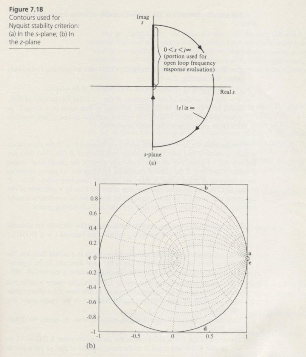
32 Discrete case ( The ideas are identical ) Unstable region of the z-plane is the outside of the unit circle Consider the encirclement of the stable region. N = { # of stable zeros } - { # of stable poles} = { n Z } { n P } = P Z Z = P N In summary,. Determine the number, P, of unstable poles of KDG. jωt 2. Plot KD(z)G(z) for the unit circle, z e and 0ωT 2π. 3. Set N equal to the net number of CCW encirclements of the point - on the plot 4. Compute Z = P N. This system is stable iff Z = 0. 54

33 55

34 ex) p. 24 (Franklin s) The unit feedback discrete system with the plant transfer function with sampling rate ½ Hz and zero-order hold G( s), ZOH at T 2 s ( s).35 ( z 0.523) Gz ( ) ( z) ( z0.35) K P 0, N # of CCW encirclements of the point 0 Z 0 56

35 Imaginary Axis Nyquist plot from Example using contour Real Axis 57

36 DESIGN SPEC. IN THE FREQUENCY DOMAIN Gain Margin (GM) : The factor by which the gain can be increased before the system to go unstable Phase Margin (PM): A measure of how much additional phase ex) p. 243 lag or time delay can be tolerated in the loop before instability results. G( s) with ZOH at T 0.2 sec 2 s ( s) ( ) ( z3.38) ( z0.242) Gz ( ) ( 0.887) 2 z z K 58

37 Bode plot Nyquist plot GM=.8, PM=8 59

38 4. INTRODUCTION An open-loop (direct) system operates without feedback and directly generates the output in response to an input signal. Open loop system with a disturbance input An closed-loop system uses a measurement of the output signal and a comparison with the desired output to generate an error signal that is used by the controller to adjust the actuator. Closed loop system with a disturbance input

39 4.2 ERROR SIGNAL ANALYSIS When H(s) =, Loop gain Sensitivity function Complementary sensitivity function Error minimization S(s), C(s): function of G c (s) and G(s) How? Design compromise

40 SENSITIVITY FUNCTION Tracking error performance Stability robustness stability E( s) R( s) D( s) G( s) E( jω) R( jω) D( jω) G( jω) S( jω) R( jω) sensitivity function Remarks: i) T( jω) Djω ( ) Gjω ( ) Djω ( ) Gjω ( ) complementary sensitivity function ii) T( jω) S( jω) 62

41 VGM Im D( jω) G( jω) plane ( DG) S GM PM - Re VGM : vector gain margin S S min( DG) the distance of the closest point from - VGM S VGM max S S S 63

42 PERFORMANCE E S R eb where eb is an error bound R S e b Define W ( ω) R performance frequency function e b S W W DG S Remark: At every frequency, the point DG W - on the Nyquist plot lies outside the disk of the center -, radius W ( jω). DG 64

43 If the loop gain is large DG S where S DG DG W DG ex) e 0.005, R below 00Hz b 0 ω 2πf 200π R e b = W W ( ω) DG 200 ω The higher the magnitude curve at low frequency, the lower the steady-state errors 65

44 ROBUST STABILITY G( jω) G ( jω)[ w ( ω) ( jω)] 0 2 G( jω) G ( jω) w ( ω) ( jω) 0 2 multiplicative uncertainty additive uncertainty where G ( s) : nominal transfer function w ( ω) : magnitude ( jω) : phase ( jω) w ( ω) W ( ω) upper bound W ( ω) : robust stability frequency function 66

45 ( ) s B ω K Gs s s s B ω ω s ω K s s s B ω ω 2 ( ) s ω w ω s s B ω ω ex) p. 250 small for low frequencies and large for high frequencies

46 0 2 Fig.7.26 Model uncertainty for disk read/write head assembly Fig.7.27 Plot of typical plant uncertainty

47 Define T( jω) S( jω) DG 0 complementary sensitivity function Assume that the nominal system is stable, DG0 0 S DG 0 (for stability robustness) DG [ w ] DG DG 0 ( DG0) w2 0 DG0 ( DG )( Tw ) 0 Suff & Nec. Cond. Tw not to be zero any w W T w T W

48 T DG since DG DG W 2 is small for high frequencies. DG 0 W robust performance 200 Bode plot robust stability W 2 ω 70

49 Remark: WT 2 W DG 2 0 DG 0 ω W DG DG Im - DG 0 W DG 2 0 Re Remark: At every frequency, the critical point, -, lies outside the disk of the center DG, radius W ( jω) Djω ( ) G( jω). 2 7

50 Robust Performance W Im - DG 0 W DG 2 0 Re Remark: For each frequency ω, construct two closed disks; one with center -, radius radius W ( jω) ; the other with center DG, radius W ( jω) D( jω) G( jω). 2 Then robust performance holds iff for each ω, these two disks are disjoint. 72

51 Bode plot 73

52 Remark: T st z e z 2 T 2 2 z ω T z s s bilinear rule There exists big difference in the Bode diagram at the high frequency. Types of Compensator: phase-lead ( high pass ~ PD) transient response phase-lag ( low pass ~ PI ) steady-state response PID : a special case of a phase lead-lag compensator 74

53 Remark: Transient response PM ς 00 Steady-state response 75 Type 0 system 20 log K at the low-frequency magnitude in Bode log-magnitude plot p Type system K v is the intersection (extension of the initial -20 db/decde) with frequency axis in Bode log-magnitude plot Type 2 system K a is the intersection (extension of the initial -40 db/decde) with frequency axis in Bode log-magnitude plot

54 DESIGN PROCEDURE IN FREQUENCY. 2. Bode plot 3. Gs ( ) hold ν jω G( ν ) Gjω ( ) T ν z 2 bilinear transformation T ν Gz ( ) 2 G( ν) Assuming that the low frequency gain of D( ω) is unity, design D( ω). 2 z ω T z D( ω) Dz ( ) 4. 76

55 ex) p (Ogata's) Gs ( ) Ts e 0 s s0 δ T st e 0 s s 0 Ts ( ) ( z ) G z e 0 0 z z s s 0 s( s 0) z

56 z ( T / 2) v 0.05v ( T / 2) v 0.05v ( v) Gv ( ) 0.05v v 0.05v 0.05v 9.24 v

57 ex) p.236- (Ogata's) e Gs ( ) s Ts K s( s ) Design Specifications: phase margin: 50 velocity error constant sampling period T gain margin: at least 0db K v : 2sec Gz ( ) Ts e K z s s( s ) Kz ( ) ( z )( z 0.887) K(0.0873z ) 2 z.887z

58 z ( T / 2) v 0.v ( T / 2) v 0.v 0.v K ( ) v Gv 0. ( ) 0.v 2 0.v ( ).887( ) v 0.v v v 2 K( )( ) K( v v ) v v vv ( ) How to determine the gain K? 80

59 K lim vg ( v) G( v) K 2 v v 0 Gv ( ) D 2 2( v v ) v v v v 2( )( ) vv ( ) o From Bode plot, PM 30 and GM 4.5dB PM should be properly adjusted. What type of compensator is needed? τv GD ( v), 0 α (phase-lead compensator) ατv 8

60 82

61 Review ( p.628 ιn Νιse's): τv GD ( v) ατv φ tan τν tan ατν dφ τ ατ 2 dν ( τν) ( ατν) v φ G max ma D G D 2 τv ( τ and break frequencies from GD ( v) ) () τ α ατv α α x tan sin ( α from the required phase) (2) 2 α α j jτωmax α ( jωmax ) jατω j α ( jω max ) where G ( jω ) G( jω ) at ω. D α max max (magnitude at the peak of phase curve) (3) max Solving (2), we can obtain α. Using max (3) and (), we can determine τ. 83

62 How to design G ( v)? D φ G max D tan sin ( jω ) max α α α 2 α α α 20 log db α 0.36 o sin 28 α 0.36 At v.7, G( jω ) db v max max max.7 τ τ α τ α G D τv v ( v) GD ( v). ατv v 84

63 85

64 G G D D v ( v) v z (0 ) ( z) z z (0 ) z z.9387 z make it a difference equation! G D ( z) G( z) z ( z0.9356) z ( z )( z 0.887) z 0.008z z 2.377z.8352z C( z) 0.089z 0.008z Rz ( ) z z.8460z ( z0.9357)( z0.845) ( z 0.826)( z j0.396)( z j0.396) 86

65 87

66 HOMEWORK 4 (DUE DATE: MAY 7TH) B-4- B-4-3 B-4-5 B-4-6 B-4-8 B-4-9 B-4-3 B-4-4