IMPLEMENTATION AND ASSESSMENT OF THE INTERFACIAL AREA TRANSPORT EQUATION IN THE SYSTEM ANALYSIS CODE TRACE

Transcription

1 The Pennsylvania State University The Graduate School College of Engineering IMPLEMENTATION AND ASSESSMENT OF THE INTERFACIAL AREA TRANSPORT EQUATION IN THE SYSTEM ANALYSIS CODE TRACE A Thesis in Nuclear Engineering by Theodore S. Worosz 2012 Theodore S. Worosz Submitted in Partial Fulfillment of the Requirements for the Degree of Master of Science August 2012

2 ii The thesis of Theodore S. Worosz was reviewed and approved* by the following: Seungjin Kim Associate Professor of Mechanical and Nuclear Engineering Thesis Advisor Kostadin Ivanov Distinguished Professor of Nuclear Engineering Arthur Motta Professor of Nuclear Engineering and Materials Science and Engineering Chair of the Nuclear Engineering Program *Signatures are on file in the Graduate School

3 iii ABSTRACT The interfacial area concentration,, is an important geometric parameter in two-phase flow, as it describes the amount of surface area between the two phases per unit mixture volume. Conventionally, has been specified through algebraic flow regime-based correlations. However, this approach cannot capture the dynamic evolution of the interfacial structure. Alternatively,, can be specified through a transport equation that provides a dynamic prediction of the interfacial area concentration through mechanistic models for bubble coalescence and breakup. Therefore, the focus of the present study is on the implementation and assessment of the interfacial area transport equation (IATE) into the nuclear reactor system analysis code TRACE. Available TRACE frameworks are reviewed focusing on the constitutive relations for the interfacial area concentration. The pilot code TRACE-T1, which employs the one-group IATE applicable to dispersed bubbly flow, is assessed against experimental databases for vertical cocurrent upward and downward air-water two-phase flows obtained in round pipes ranging in diameters from 2.54 cm to cm. Predictions of experimental pressure, void fraction, bubble velocity, and interfacial area concentration are generated with TRACE-T1 and TRACE-NT (a non-transport version of the code) for comparison. TRACE-T1 allows for non-linear development of and demonstrates significant improvement over the non-transport approach. The TRACE- T1 code is extended to include a two-group IATE model, applicable to bubbly, slug, and churnturbulent flows in moderate diameter pipes, to establish the pilot code TRACE-T2. An overview of the selected IATE model and the details of its implementation are provided. Furthermore, the feasibility of two-group interfacial area transport in TRACE-T2 is demonstrated through predictions of two-group experimental data. Lastly, recommendations for future code development and improvements to the interfacial area transport approach are made.

4 iv TABLE OF CONTENTS LIST OF FIGURES... vi LIST OF TABLES... ix NOMENCLATURE... x ACKNOWLEDGEMENTS... xv Chapter 1 Introduction Two-Phase Flow Regimes The Two-Fluid Model Constitutive Relations for the Interfacial Area Concentration Importance of the Interfacial Area Concentration Conventional Specification of the Interfacial Area Concentration The Interfacial Area Transport Equation Nuclear Reactor Thermal-Hydraulic System Analysis Codes Thesis Objectives Chapter 2 Overview of Available TRACE Framework TRACE v TRACE v4.921b TRACE-T TRACE-T1 Interfacial Area Transport Model TRACE-T1 Input Chapter 3 Assessment of TRACE-T Pressure Predictions Void Fraction Predictions Gas Velocity Predictions Interfacial Area Concentration Predictions Chapter 4 Development of a Two-Group Interfacial Area Transport Pilot Code Summary of Two-Group Source/Sink Mechanisms Overview of Implemented Two-Group Interfacial Area Transport Model Two-Group Interfacial Area Transport Equation Two-Group Source/Sink Term Models TRACE-T2 Input Output of Two-Group Parameters Chapter 5 Assessment of TRACE-T Predictions of One-Group Conditions

5 v 5.2 Predictions of Two-Group Conditions Identification of Potential Framework Issues Specification of Interfacial Drag Intergroup Momentum Transfer Incorrect Weighting Factors Chapter 6 Summary and Recommendations Summary of the Present Work Assessment of TRACE-T Development and Assessment of TRACE-T Recommendations for Future Work REFERENCES

6 vi LIST OF FIGURES Figure 1-1: Characteristic flow regimes in co-current vertical upward air-water two-phase flow (Images adapted from Yadav, 2009) Figure 1-2: The void fraction of the k th -phase ( ) represents the volume of the k th -phase per unit mixture volume Figure 1-3: Characteristic bubble groups in the two-group IATE (Ishii et al., 2009) Figure 2-1: Pre-CHF flow regime map for interfacial heat transfer (TRACE v5.0 Theory Manual, 2007) Figure 2-2: Schematics of one-group interfacial area transport equation source/sink mechanisms Figure 2-3: Pipe models for (a) TRACE-NT and (b) TRACE-T Figure 3-1: Vertical co-current upward air-water two-phase flow assessment conditions in various inner diameter round pipes (Ishii et al., 2002b; Ishii et al., 2010a; Ishii et al., 2010b) Figure 3-2: Vertical co-current downward air-water two-phase flow assessment conditions in a 2.54 cm inner diameter round pipe (Ishii et al., 2002b) Figure 3-3: Vertical co-current downward air-water two-phase flow assessment conditions in a 5.08 cm inner diameter round pipe (Ishii et al., 2002b) Figure 3-4: Characteristic pressure predictions for vertical co-current upward flow; Run 4-4 (j g = m/s and j f = m/s). ±5% error bars shown Figure 3-5: Characteristic pressure predictions for vertical co-current downward flow; Run 1d-4 (j g = m/s and j f = m/s). ±5% error bars shown Figure 3-6: Void fraction predictions for Run 8-2 (j g = m/s and j f = m/s). ±10% error bars shown Figure 3-7: Void fraction predictions for Run 1d-5 (j g = m/s and j f = m/s). ±10% error bars shown Figure 3-8: Bubble velocity predictions for Run 2-6 (j g = m/s and j f = m/s). ±10% error bars shown Figure 3-9: Bubble velocity predictions for Run 1d-3 (j g = m/s and j f = m/s). ±10% error bars shown

7 vii Figure 3-10: (a) Interfacial area concentration predictions made by TRACE-T1, TRACE- NT, and MATLAB for a pressure dominated condition, Run 2-4 (j g = m/s and j f = m/s). (b) Source/sink contributions from the MATLAB script. ±10% error bars shown Figure 3-11: (a) Interfacial area concentration predictions made by TRACE-T1, TRACE- NT, and MATLAB demonstrating nonlinear development, Run 1-11 (j g = m/s and j f = m/s). (b) Source/sink contributions from the MATLAB script. ±10% error bars shown Figure 3-12: (a) Opposing trends in TRACE-T1 and TRACE-NT predictions for decreasing interfacial area concentration in vertical-upward flow, Run 8-2 (j g = m/s and j f = m/s). (b) Source/sink contributions from the MATLAB script showing random collision coalescence as the dominant mechanism. ±10% error bars shown Figure 3-13: (a) Opposing TRACE-T1 and TRACE-NT predictions for increasing interfacial area concentration in vertical co-current downward flow, Run 1d-5 (j g = m/s and j f = m/s). (b) Source/sink contributions from the MATLAB script showing turbulence impact breakup as the dominant mechanism. ±10% error bars shown Figure 4-1: Two-group source/sink term nomenclature Figure 4-2: Schematics of intra- and intergroup bubble expansion/contraction Figure 4-3: Schematics of intra- and intergroup random collision bubble interaction mechanisms Figure 4-4: Schematics of intra- and intergroup wake entrainment bubble interaction mechanisms Figure 4-5: Schematics of intra- and intergroup turbulence impact bubble interaction mechanisms Figure 4-6: Schematic of the surface instability bubble interaction mechanism Figure 4-7: Schematic of the shearing-off bubble interaction mechanism Figure 4-8: Bivariate distribution in bubble volume of group-1 bubbles used to develop the generalized intra- and intergroup random collision and wake entrainment source terms (Fu, 2001) Figure 4-9: Behavior of bubble (a) surface area and (b) volume changes for generalized group-1 coalescence interactions Figure 4-10: Comparison of PIPE models for TRACE-NT, TRACE-T1, and TRACE-T

8 Figure 5-1: Void fraction predictions made by TRACE-T2, TRACE-T1, and TRACE-NT for a one-group condition, Run 2-16 (j g = m/s and j f = m/s). ±10% error bars shown Figure 5-2: Interfacial area concentration predictions made by TRACE-T2, TRACE-T1, and TRACE-NT for a one-group condition, Run 2-16 (j g = m/s and j f = m/s). ±10% error bars shown Figure 5-3: Group-1 interfacial area concentration source/sink contributions calculated in TRACE-T2 for Run 2-16 (j g = m/s and j f = m/s). ±10% error bars shown Figure 5-4: (a) Group-1 (G1) and group-2 (G2) void fraction predictions made by TRACE-T2. (b) Total void fraction predictions made by TRACE-T2, TRACE-T1, and TRACE-NT. Run 2-10 (j g = m/s and j f = m/s). ±10% error bars shown Figure 5-5: Group-1 (G1) and group-2 (G2) interfacial area concentration predictions made by TRACE-T2, Run 2-10 (j g = m/s and j f = m/s). ±10% error bars shown Figure 5-6: Total interfacial area concentration predictions made by TRACE-T2, TRACE-T1, and TRACE-NT. Run 2-10 (j g = m/s and j f = m/s). ±10% error bars shown Figure 5-7: Total interfacial area concentration source/sink contributions from TRACE- T2 for Run 2-10 (j g = m/s and j f = m/s) source. ±10% error bars shown Figure 5-8: (a) Group-1 (G1) and group-2 (G2) void fraction predictions made by TRACE-T2. (b) Total void fraction predictions made by TRACE-T2 and TRACE- NT. Run 2-12 (j g = m/s and j f = m/s). ±10% error bars shown Figure 5-9: (a) Group-1 (G1) and group-2 (G2) interfacial area concentration predictions made by TRACE-T2. (b) Total interfacial area concentration predictions made by TRACE-T2 and TRACE-NT. Run 2-12 (j g = m/s and j f = m/s). ±10% error bars shown Figure 5-10: Group-1 (G1) and group-2 (G2) bubble velocity predictions made by TRACE-T2, Run 2-12 (j g = m/s and j f = m/s). ±10% error bars shown Figure 5-11: Group-1 (G1) and group-2 (G2) interfacial area concentration predictions made by TRACE-T2 and the two-group MATLAB program utilizing (a) drift-flux relations and (b) interpolated TRACE-T2 velocity solutions for the group velocities, Run 2-12 (j g = m/s and j f = m/s). ±10% error bars shown Figure 5-12: (a) Group-1 (G1) and group-2 (G2) interfacial area concentration predictions made by TRACE-T2 demonstrating the inactivity of intergroup random collision and wake entrainment. (b) Close-up view of the group-2 prediction showing the lack of group-2 generation. Run 4-7 (j g = m/s and j f = m/s). ±10% error bars shown viii

9 ix LIST OF TABLES Table 2-1: One-group IATE model coefficients implemented into TRACE-T1 for vertical upward and vertical co-current downward flow configurations in round pipes Table 3-1: Summary of round pipe experimental databases and axial measurment locations Table 4-1: Two-group source/sink mechanisms (G1 = group-1; G2 = group-2) Table 4-2: Two-group model parameters for vertical upward flow implemented into TRACE-T

10 x NOMENCLATURE Latin Characters () interfacial area concentration average surface area of particles of volume shear coefficient IATE source/sink coefficient; other coefficients film roughness parameter particle drag coefficient interfacial drag coefficient distribution parameter pipe diameter; other diameters as indicated by subscript hydraulic diameter volume equivalent diameter of a particle with volume ( = (6 ) / ) surface equivalent diameter of a particle with surface area ( = ( ) / ) h h h h internal energy distribution function; force per unit volume; friction factor gravitational acceleration body force mass flux heat transfer coefficient; enthalpy interfacial heat transfer coefficient for the k th -phase to the interface vapor enthalpy of the bulk vapor if the vapor is condensing or the vapor saturation enthalpy if liquid is vaporizing liquid enthalpy of the bulk liquid if the liquid is vaporizing or the liquid saturation enthalpy if vapor is condensing general interfacial transfer term

11 xi L/D superficial velocity of the k th -phase length to diameter ratio Laplace length ( = /Δ) generalized interfacial drag force number density viscosity number = Δ pressure profile slip factor partial pressure of the vapor heat transfer rate per unit volume heat flux power deposited directly to the gas or liquid radius number source/sink rate Reynolds number particle source/sink rate due to the j th -type interaction time temperature saturation temperature corresponding to the vapor partial pressure velocity drift-velocity turbulent fluctuation velocity particle volume ratio of minimum to maximum slug bubble volume ( =, /, ) Weber number

12 xii Greek Characters Δ Φ void fraction mass generation rate intergroup mass transfer rate from group-1 to group-2 turbulent energy dissipation rate net volume transfer from group-1 to group-2 due to the j th -interaction mechanism liquid film velocity reduction factor dynamic viscosity kinematic viscosity ratio of average to maximum bubble diameter generated in shearing-off density surface tension stress tensor two-phase multiplier source/sink term due to the j th -type interaction mechanism intergroup transfer coefficient shape factor Subscripts and Superscripts 2 ; two-phase bubble continuous phase; bubble at group boundary critical droplet; dispersed phase standard drag

13 xiii h ; dispersed bubbles or transition void fraction from dispersed bubbly flow expansion/contraction liquid gas mixture interface isotropic index indicating phase, bubble group, or field large bubbles mixture maximum phase change pressure drop relative random collision surface instability Sauter-mean shearing-off turbulent turbulence impact total water vapor wall; wake wake entrainment

14 xiv Mathematical Notation and Operators / / vector quantity scalar quantity total derivative substantial derivative with respect to the k th -phase velocity area-average of void-weighted area-average of interfacial area concentration-weighted area-average of phase-average of mass-weighted mean value of

15 xv ACKNOWLEDGEMENTS In the course of our lives, we reach many milestones through hard work, perseverance, and the help of those around us. As such, the author would like to thank those that led to the completion of this work. The author expresses his sincerest gratitude to his advisor, Dr. Seungjin Kim. Dr. Kim s passion for learning and dedication to his students is surpassed by few, and his rigorous pedagogy is a great asset to training the engineers of tomorrow. The author is grateful for the opportunity to study two-phase flow under his direction and thanks him for his continued guidance. The author also thanks Dr. Ivanov and Dr. Motta for reviewing the manuscript and providing valuable suggestions. Additionally, the author thanks the United States Nuclear Regulatory Commission for its financial support of the author s graduate studies through the NRC Fellowship Program. The author is very fortunate to be a member of the Advanced Multi-Phase Flow Laboratory and has the greatest respect for all of the members. In particular, the author extends special thanks to Dr. Justin D. Talley, who worked closely with the author during the course of this work and provided invaluable mentorship. Mr. Mohan Yadav is also recognized for his continued advice and technical prowess. Additionally, the author thanks Mr. Matt Bernard for his programming expertise and many valuable discussions. The author is also very grateful to his family and friends for their support throughout his life. In particular, the author thanks his parents, Susan and Stan, for instilling in him many of the traits and values that enabled him to pursue this work. The author also thanks his two younger brothers, Chris and Matt, for their continued encouragement and inspiration through their own great achievements. Lastly, the author thanks his girlfriend, Miss Tiffany Bennett, for her unconditional love and support throughout the years.

16 This thesis is dedicated to my parents. xvi

17 1 Chapter 1 Introduction Multiphase or multicomponent flows involve the flow of two or more phases or components. These flows occur in many manufacturing processes, power generation systems, the environment, and even in the home or office. Boilers, internal combustion engines, aerosol coatings, a carbonated beverage, water-jet cutting systems, sewage, a pot of boiling water, and sediment transport are just a few examples of these flows. Thus, the study of multiphase/multicomponent flows is a relevant topic in many disciplines. In particular, gas-liquid two-phase flows have been studied in great detail by the nuclear energy, chemical manufacturing, and other energy industries due to their impact on the safety and efficiency of various systems and processes. Gas-liquid two-phase flows are characterized by the presence of multiple deforming interfaces that form a complex, dynamic interfacial structure (Ishii and Hibiki, 2006). The surface area of the interface is a critical parameter in the study of two-phase flow, as the transfers of mass, momentum, and energy between the two phases are related to the available area between them. The interfacial area concentration,, which is defined as the surface area of the interface per unit mixture volume, provides a measure of the interfacial surface area and is thus a fundamental geometric parameter of two-phase flow (Ishii and Hibiki, 2006). In view of the importance of the interfacial area concentration, the main objective of this thesis is to implement and assess the interfacial area transport equation in the United States Nuclear Regulatory Commission s system analysis code, TRACE. Before elaborating on the specific objectives of this thesis, however, necessary background information on the analysis of two-phase flow is presented to further motivate the importance of the interfacial area concentration.

18 2 1.1 Two-Phase Flow Regimes Analogously to the classification of single-phase flows as laminar and turbulent, twophase flows are characterized according to the interfacial structures present in the flow (Ishii and Hibiki, 2006). The macroscopic configuration of the interfacial structure is commonly classified into different flow regimes, which are strongly dependent on the channel geometry, flow rate of each phase, and fluid properties. In this context, macroscopic refers to the global interfacial structure viewed from the system scale perspective (e.g. flow patterns throughout a pipe). To provide a physical sense of gas-liquid two-phase flow, Figure 1-1 shows examples of characteristic flow regimes in vertical co-current upward air-water two-phase flow. Considering the images from left to right, at lower gas flow rates, small, near-spherical bubbles are dispersed throughout a continuous liquid. This configuration is classified as the bubbly flow regime. With increasing gas flow rate, bubbles coalesce to form larger distorted bubbles, and additional coalescences will eventually lead to the formation of larger spherical-cap shaped bubbles. If the flow is bounded by a channel wall, large, periodic, elongated slug bubbles that occupy nearly the entire cross-section will result due to the wall shear and additional coalescence. The slug bubbles are followed by highly active liquid regions called liquid slugs that contain numerous smaller bubbles. These flow characteristics represent the slug flow regime. Further increasing the gas flow rate can result in the churn-turbulent flow regime, which is characterized by large churning regions of gas and liquid. Finally, for higher gas flow rates, a continuous gas core develops that is surrounded by a liquid film. Droplets and ligaments of liquid can flow in the gas core as well, yielding a very complex interfacial structure. This is characteristic of the annular flow regime. Clearly, the dynamics of the flow will be different in each flow regime due to the presence of different interfacial structures. Furthermore, for heated flows, each flow regime will have different heat transfer characteristics between the phases and heated surfaces in the system. For

19 3 example, for a given mass of vapor, a bubbly flow will have improved heat transfer compared to a slug flow due to greater interfacial area concentration. These considerations are particularly important in the design and analysis of energy systems where thermal limits on various structural materials (e.g. fuel cladding in a nuclear reactor core) must be met. Additional discussion on various flow regimes can be found throughout the literature (Rouhani and Sohal, 1982; Mishima and Ishii, 1984; Dukler and Taitel, 1986). Bubbly Slug Churn-Turbulent Annular Figure 1-1: Characteristic flow regimes in co-current vertical upward air-water two-phase flow (Images adapted from Yadav, 2009). 1.2 The Two-Fluid Model The analysis of gas-liquid two-phase flows is based in the constructs of classical continuum mechanics. The governing equations of mass, momentum, and energy hold within each distinct phase, and appropriate balance laws can be written at the interfaces that separate the phases. However, the presence of multiple, deforming interfaces yields an immensely complicated multi-boundary problem that is far from tractable even for the simplest of flows.

20 4 Therefore, in practical analyses, two-phase flows are considered in an average sense, which can be thought of as a flow of interpenetrating continua. Various averaging techniques (e.g. volume, time, ensemble, etc.) have been applied to the local instantaneous balance equations to derive average field equations for each phase. Similar forms of the governing equations result from the different averaging processes, with the major differences being the interpretation of the averaged variables (Ishii and Hibiki, 2006; Drew and Passman, 1999). Perhaps the most well-known example of these averaged balance laws is the timeaveraged two-fluid model developed by Ishii (1975). A simplified form of the two-fluid model that can be applied in most practical analyses is given as (Ishii and Hibiki, 2006): + ( ) = [1-1] + ( ) = [1-2] ( ) h + h = h + + [1-3] Equations [1-1], [1-2], and [1-3] represent the average balances of mass, momentum, and energy (enthalpy), respectively, within the k th -phase (k=1 or 2). Although a formulation of the average entropy inequality is available, it is not presented here in this brief summary of the twofluid model. The double over-bar and hat denote the phase-average and mass-weighted mean values, respectively. is the void fraction of the k th -phase, which is pictorially shown in Figure 1-2 to represent the volume of k th -phase per unit mixture volume. Alternatively, can be interpreted as the probability that a point is occupied by the k th -phase.,,,,, and

21 are the velocity, density, pressure, viscous stress tensor, turbulent stress tensor, and body force for the k th -phase. Likewise, h,,, and are the enthalpy, conduction heat flux, turbulent heat flux, and viscous dissipation rate for the k th -phase. These terms have analogous interpretations to those found in the governing equations of single-phase flow. and are the mass generation rate and generalized interfacial drag force for the k th -phase. The subscript i signifies the interface, and thus, the terms:,,, h, and are the velocity, shear stress, pressure, and heat flux at the interface. The quantity is the interfacial area concentration, which physically represents the amount of interfacial surface area per unit mixture volume. 5 Figure 1-2: The void fraction of the k th -phase ( ) represents the volume of the k th -phase per unit mixture volume. In addition to the balance laws within each phase, the balance laws of the interface must also be satisfied. Thus, from an average of the local instantaneous jump conditions (interfacial balance laws), the following macroscopic jump conditions that constrain the interfacial transfer terms in Equations [1-1] [1-3] are given as (Ishii and Hibiki, 2006):

22 6 = 0 [1-4] = [1-5] h + = 0 [1-6] Physically, Equation [1-4] indicates that mass is conserved across the interface; the mass generation process results in a loss from one phase and an equal gain by the other. Similarly, Equation [1-5] asserts that the interfacial surface forces that are represented by the generalized drag term are equal and opposite between the phases. Likewise, Equation [1-6] affirms conservation of energy between the phases across the interface. As with the governing equations of single-phase flow, the average balance equations presented above are not closed by themselves. Constitutive equations are required to relate unknown quantities to the fundamental variables of choice, and empirical data is relied upon to determine coefficients that describe microscopic material behavior (e.g. density, dynamic viscosity, surface tension, etc.). Drew and Lahey (1979) provide detailed discussion on both the formal and phenomenological approaches to developing the constitutive equations in the twofluid model. Extensive development of this topic is also presented by Ishii and Hibiki (2006). The two-fluid model can provide a detailed treatment of a wide range of two-phase flow phenomena compared to simpler mixture formulations such as the homogenous equilibrium model (Wallis, 1969) or drift-flux model (Zuber and Findlay, 1965), as it allows for both mechanical and thermal non-equilibrium between the phases. Although the two-fluid model is a

23 7 higher fidelity model, its accuracy is still limited by the validity of the constitutive relations supplied to it. One cannot expect greater accuracy than the combined accuracies of the various constitutive relations that are required to close the system of equations. Specifically, the two-fluid model requires the development of additional closure models to the ones used in single-phase flow analysis due to the additional terms accounting for the transfers of mass, momentum, and energy across the interface. Furthermore, obtaining accurate closure for the interfacial area concentration is of particular importance because the interfacial area concentration provides information about the interfacial structure of the flow. 1.3 Constitutive Relations for the Interfacial Area Concentration Importance of the Interfacial Area Concentration In the two-fluid model (Ishii, 1975), interaction terms appear in the field equations that couple the phases together through the transport of mass, momentum, and energy across the interface. In general, the interfacial transfer terms are directly related to the interfacial area concentration and to driving forces that describe the local transport mechanisms such that (Ishii and Mishima, 1984): = [1-7] Where is a general interfacial transfer term. For example, the standard drag force component of the generalized interfacial drag term written for the dispersed phase,, can be expressed as (Ishii and Mishima, 1984):

24 8 = 4 [1-8] 2 Here, and are the particle drag coefficient and the relative velocity between the dispersed and continuous phases, respectively. The ratio of the Sauter-mean radius,, to the drag radius,, represents a shape factor; for spherical dispersed phase particles, this ratio is unity. The interfacial area concentration is a length scale of the interface that describes the geometric capacity for interfacial transport. The amount or degree of transport of mass, momentum, and energy across the interface is proportional to the amount of surface area available for interaction between the phases (Ishii and Hibiki, 2006). Thus, the transport characteristics vary as the interfacial structure changes. The interfacial area concentration is a fundamental geometric parameter of two-phase flow that provides information about the configuration of the interfacial structure Conventional Specification of the Interfacial Area Concentration Conventionally, the interfacial area concentration has been specified through algebraic, flow regime dependent correlations developed from limited ranges of experimental data (Ishii et al., 2009). Examples of several empirical correlations are summarized by Delhaye and Bricard (1994), where the interfacial area concentration is related to global flow parameters, such as pressure drop and flow rates. While the interfacial area concentration is related to these parameters, it also strongly depends on system geometry as well as on the void fraction (Ishii and Mishima, 1980). Thus, one cannot expect generality from correlations of global flow parameters, as was demonstrated in Delhaye and Bricard s (1994) study. Thus, this approach to specifying the interfacial area concentration is limited to specific systems and ranges of operating conditions.

25 9 Using a mechanistic modeling approach, Ishii and Mishima (1980) developed expressions for the interfacial area concentration for bubbly, slug, churn-turbulent, and annular flows. For slug/churn-turbulent and annular flows, respectively, the interfacial area concentration is given as: = [1-9] 1 1 = [1-10] 1 1 In a bubbly flow, the overall average void fraction, is equal to the average void fraction in the liquid slug section,, and thus, Equation [1-9] reduces to a linear relationship between and the void fraction ( = 3 ). Although derived from geometric considerations, Equations [1-9] and [1-10] still require one to know the flow regime and, thus, cannot capture the true evolution of the interfacial structure alone. Additionally, estimates for,, (the liquid droplet fraction), and (the film roughness parameter) are required to complete the specification of the interfacial area concentration with these models. It is also noted that conventional relationships such as these provide an estimate of an average value of the interfacial area concentration within the flow, not a local value. This is mainly because available measurement techniques, such as chemical absorption and photographic methods, were limited to obtaining volume-averaged estimates of the interfacial area concentration, and consequently, analysis methods focused on the gross, average behavior of a system. Only relatively recently have databases been established with detailed local measurements of the interfacial area concentration to assist multidimensional model development (Kataoka, 2010).

26 The Interfacial Area Transport Equation An alternative approach to the conventional flow regime-based methodology is to utilize a transport equation to specify the interfacial area concentration. The comprehensive mathematical formulation of the interfacial area transport equation (IATE) can be found in the work by Ishii and Kim (2004) and is presently summarized. Similar approaches to the treatment of the interfacial area concentration can also be found in the literature (Guido-Lavalle et al., 1994; Kocamustafaogullari and Ishii, 1995; Millies et al., 1996; Morel et al., 1999). It is noted that since the present work focuses on two-phase flows consisting of dispersed gas in a continuous liquid, the model is presented with the gas as the dispersed phase, and the terms bubble and particle are used interchangeably. However, this does not detract from the generality of the interfacial area transport approach in application to other flows with dispersed, interacting particles (e.g. droplets). Since the interfacial area of fluid particles is closely related to the number of particles, the interfacial area transport equation can be formulated in a manner analogous to the Boltzmann transport equation. Define (,,, ) to be the particle number density distribution function per unit mixture and bubble volume. This distribution function, which is assumed to be continuous, specifies the probable number density of particles at position within a spatial volume that are moving with particle velocity within with particle volume within at time. Assuming that the change in particle velocity is small within the time interval to +, one can obtain the following transport equation for the distribution function (,, ): + () + = + [1-11]

27 11 Here, / denotes a total derivative. In Equation [1-11], and represent the particle source/sink rates per unit mixture and bubble volume due to the j th -type particle interaction (i.e. disintegration or coalescence mechanisms) and due to phase change, respectively. From the distribution function (,, ), the particle number per unit mixture volume, void fraction, and interfacial area concentration are defined, respectively, as: (, ) (,, ) [1-12] (, ) (,, ) [1-13] (, ) (,, ) () [1-14] where () is the average surface area of particles with volume. By integrating Equation [1-11] over all particle volumes, a transport equation for the particle number density (number per unit mixture volume) is obtained as: + = + [1-15] Where the average local particle velocity is defined to be: (, ) (,, )(,, ) [1-16] (,, )

28 12 The terms and represent the number source/sink rates per unit mixture volume due to the j th -type particle interaction and due to phase change, respectively. Thus, the number source/sink rate is defined as: (, ) (,, ) [1-17] Multiplying Equation [1-11] by the particle volume and integrating over all particle volumes, the void transport equation is found to be given as: + Γ = + [1-18] Where the average center-of-volume gas velocity is defined to be: (, ) (,, )(,, ) (,, ) [1-19] The term is the volume generation rate per unit mixture volume due to the nucleation source, which is defined by: [1-20] Lastly, the interfacial area transport equation can be obtained by multiplying Equation [1-11] by () and integrating over the particle volume range: + ( ) = [1-21]

29 13 Where the interfacial velocity is defined as: (, ) (,, ) ()(,, ) (,, ) () [1-22] It can be shown that the particle number density can be approximated as: = [1-23] Where the shape factor, which is found in Equation [1-21], is defined by: = 1 36 [1-24] Here, and are the Sauter-mean and volume equivalent diameters, respectively. The left hand side of Equation [1-21] represents the total rate of change of the interfacial area concentration due to the local time rate of change and to advection. The first term on the right hand side represents the change in interfacial area concentration due to expansion, contraction, and/or phase change excluding nucleation. The second term represents the sources and sinks of interfacial area concentration due to particle interactions leading to coalescence and breakup. The last term represents the interfacial area concentration source due to nucleation, where is the bubble diameter for a given nucleation process (Ishii and Kim, 2004). As shown in Figure 1-1, a wide range of bubble sizes and shapes can exist depending on the flow regime. In the formulation presented above, the transport equation was integrated over all particle volumes under the assumption that the sizes, shapes, (i.e. the average particle surface area) and transport phenomena of the particles are similar over the entire particle volume range. While this assumption holds for dispersed bubbly flows where the bubbles remain nearly

30 14 spherical, it breaks down when larger cap-shaped bubbles are present in the flow. The different bubble sizes and shapes in general two-phase flows cause substantial differences in the bubbles transport characteristics, including interfacial drag and bubble interaction mechanisms. Thus, a multi-group approach is required to treat a wide range of two-phase flow conditions. Currently, in view of their drag characteristics and interaction phenomena, bubbles are categorized into two characteristic groups (Ishii and Kim, 2004). Group-1 includes small spherical and distorted bubbles, while group-2 includes cap, slug, and churn-turbulent bubbles. To obtain the two-group transport equations for particle number, void fraction, and interfacial area concentration, Equation [1-11] is integrated separately over the volume range of each group. The boundary between the two groups is defined by the critical bubble volume,, which is specified through the maximum distorted bubble limit,,, given by Ishii and Zuber (1979) as:, = 4 Δ [1-25] This diameter is determined from the interfacial drag correlations for distorted and cap-bubbles (Ishii and Zuber, 1979). A schematic of the bubble categorization scheme is shown in Figure 1-3. Figure 1-3: Characteristic bubble groups in the two-group IATE (Ishii et al., 2009).

31 15 With these considerations, the two-group interfacial area transport equation is given as (Ishii and Kim, 2004): Group-1: + ( ) = 2 3 ( ) + +, + [1-26] Group-2: + ( ) = ( ) + +, + [1-27] where the subscripts 1 and 2 denote group-1 and group-2, respectively. In Equations [1-26] and [1-27], the non-dimensional parameter is a measure of the average size of group-1 bubbles with respect to the size at the group boundary and is defined as: =, [1-28] Where is the bubble diameter at the group boundary. Additionally, the coefficient accounts for the intergroup transfer at the group boundary between the two groups due to expansion/contraction., and, are the interfacial area concentration sources/sinks due to the j th -type bubble interaction mechanism and due to phase change for the k th bubble group, respectively. In order to utilize the two-group interfacial area transport equation, it is necessary to track the distribution of the total void fraction between the groups. This is important because the bubble interaction mechanisms that act as sources or sinks to the interfacial area concentration are

32 16 functions of the group void fractions. Hence, either void transport equations or continuity equations with additional mass sources to account for intergroup transfer due to particle interactions are required for each group. The intergroup mass transfer rate from group-1 to group- 2, Δ, is given as (Ishii and Hibiki, 2006): Δ =, + ( ) + [1-29] Where, describes the net volume transfer from group-1 to group-2 due to the j th -type bubble interaction. To close the one-group and two-group interfacial area transport equations, models are required for the source/sink terms that account for changes in the interfacial area concentration due to various bubble coalescence and breakup mechanisms as well as phase change. In the twogroup formulation, additional models are needed for the mass transfer between the groups due to intergroup interactions. Furthermore, specification of the interfacial velocity for the k th -group,, is required. 1.4 Nuclear Reactor Thermal-Hydraulic System Analysis Codes From the inception of a nuclear reactor s design, detailed neutronic and thermal-hydraulic analyses are required to ensure safe and economic operation of the plant. To perform these analyses, various computer codes are relied upon to solve the governing mathematical models of the plant s systems with various degrees of fidelity. Thermal-hydraulic system analysis codes are used to analyze overall system behavior, such as flow through the primary and secondary loops of a pressurized water reactor. When coupled with neutronics calculations, these codes provide an invaluable tool in assessing plant dynamics under normal operation and accident scenarios. Some

33 17 examples of system analysis codes include TRAC (Spore et al., 1993), RELAP5-3D (RELAP5-3D Code Manual, 2005), CATHARE (Barre and Bernard, 1990), and TRACE (TRACE v5.0 Theory Manual, 2007). TRACE, the TRAC/RELAP Advanced Computational Engine, is the United States Nuclear Regulatory Commission s (NRC) consolidated neutronic-thermalhydraulic system analysis code. An overview of the TRACE framework is presented in Chapter 2, as it is the base code used in this thesis. In current nuclear reactor thermal-hydraulic system analysis codes, such as TRACE and RELAP5-3D, a flow regime-based constitutive equation package is used to close the two-fluid model field equations. Specifically, the interfacial area concentration is calculated using conventional algebraic relations (TRACE v5.0 Theory Manual, 2007; RELAP5-3D Code Manual, 2005). Mortensen (1995) and Kelly (1997) identified several shortcomings related to the static, flow regime-based approach, which can be summarized as follows: Since the flow regime transition criteria are algebraic relations for steady-state, fullydeveloped flows, they reflect neither the true dynamic nature of changes in the interfacial structure, nor the gradual regime transition. Significant errors in code predictions can be introduced by the compounding effects of the two-step flow regime-based method. The existing flow regime dependent correlations and criteria are only valid in limited parameter ranges for certain operational conditions. Often the geometrical scale effects are not taken into account correctly. Hence, these models may cause significant discrepancies, artificial discontinuities, and numerical instabilities. In the flow regime-based approach, the flow regime is first identified based on static transition criteria (e.g. a void fraction or flow rate limit). Then, appropriate constitutive relations for the flow regime are selected to close the two-fluid model. This approach suffers from several

34 18 aspects. Physically, the development of the interfacial structures and hence flow regime transition is a dynamic, continuous process that cannot be captured through fixed transition criteria. Flow regime transitions gradually occur in regions around these boundaries, and as such, an inherent level of uncertainty is introduced by describing flow regime transitions as instantaneous. Furthermore, the interfacial structure is dependent on the channel geometry, which cannot be captured in general by a simple set of flow regime transition criteria. Additionally, flow regime specific correlations can be discontinuous at the flow regime boundaries, which can lead to artificial bifurcations and numerical oscillations in thermal-hydraulic analyses. This can lead to additional uncertainty due to numerical treatments that are used to smooth the transitions between the different closure relations employed in each regime. The interfacial area transport equation is a promising alternative to the flow regime-based approach, as it can provide a continuous prediction of the interfacial area concentration, which can be used to characterize the interfacial structure. In this way, the static regime transition criteria can be eliminated, and more mechanistic closure models can be applied that reflect the true nature of the interfacial structure. Thus, the numerical issues near flow regime transitions can be reduced. Some efforts have been made to incorporate the interfacial area transport equation into system analysis codes to provide a dynamic estimate of the interfacial area concentration. Ishii et al. (2000) examined the feasibility of implementing the one-dimensional, one-group interfacial area transport equation into the system analysis code TRAC. Improved predictions of the interfacial area concentration using the transport equation over conventional relations were demonstrated. However, comparisons to experimental data from only a limited number of flow conditions were used to validate the preliminary implementation. Schilling (2007) implemented the two-group interfacial area transport model of Smith (2002) into an experimental version of TRACE that contained an existing framework for a droplet field with an interfacial area transport

35 19 equation. Several difficulties were enumerated in the assessment of the implementation, and a fully functional two-group code capable of predicting experimental data was not attained. In view of this, Kim and Talley (2009) adopted a systematic approach and successfully implemented the one-group interfacial area transport equation into the framework developed by Schilling (2007). Improvements in the prediction capabilities of the interfacial area concentration compared to the conventional approach in TRACE were demonstrated. However, additional assessment of the implementation is required to validate the code against a wide range of bubbly flow conditions. Furthermore, development of a functioning two-group interfacial area transport pilot code is required to extend the range of applicability of the code beyond the bubbly flow regime. 1.5 Thesis Objectives The previous sections have introduced the relevance of gas-liquid two-phase flow and motivated the importance of a dynamic model for the interfacial area concentration to provide consistent closure of the two-fluid model. In view of the appeal to apply this dynamic approach to nuclear reactor thermal-hydraulic system analysis codes, the objectives of the present thesis are as follows: 1. Review available TRACE frameworks focusing on the specification of the interfacial area concentration. 2. Assess the implementation of the adiabatic, one-dimensional, one-group interfacial area transport equation in TRACE (Kim and Talley, 2009) against available experimental data.

36 20 3. Develop and assess a pilot TRACE code that employs the adiabatic, onedimensional, two-group interfacial area transport equation to specify the interfacial area concentration. 4. Provide direction for future work on the development of the interfacial area transport approach. These objectives are addressed in turn in the following chapters. Chapter 2 presents an overview of three available TRACE frameworks, TRACE v5.0, TRACE v4.291b, and TRACE- T1, in regards to their field equations and constitutive relations. TRACE v5.0 is the current public version of TRACE that uses a flow regime-based constitutive equation package (TRACE v5.0 Theory Manual, 2007), while TRACE v4.291b (Schilling, 2007) and TRACE-T1 (Kim and Talley, 2009; Kim et al., 2011) are experimental code versions that employ the interfacial area transport equation. To validate the implementation of the adiabatic, one-group interfacial area transport equation in TRACE-T1, code predictions are assessed against a wide range of bubbly flow experimental data in Chapter 3. The development of a functioning two-group pilot code is presented in Chapter 4. A review of the selected two-group interfacial area transport model is included, and the details of its implementation to establish the two-group pilot code, TRACE-T2, are provided. Chapter 5 presents a preliminary assessment of TRACE-T2 against available experimental data. Lastly, Chapter 6 concludes with a summary of the present thesis and provides recommendations for future work.

37 21 Chapter 2 Overview of Available TRACE Framework TRACE is the NRC s best-estimate reactor system analysis code used for analyzing transient and steady-state neutronic-thermal-hydraulic behavior in light water reactors. TRACE is the result of the consolidation of four system codes that were maintained by the NRC, namely: TRAC-P, TRAC-B, RELAP5, and RAMONA (TRACE v5.0 Theory Manual, 2007). The field equations and closure relations, specifically for the interfacial area concentration, are reviewed in this Chapter. Since extensive databases of two-phase flow parameters, including the interfacial area concentration, are currently available for adiabatic air-water two-phase flows (Ishii et al., 2009), the present study focuses on adiabatic conditions. Consequently, although the energy equations are presented for completeness, the details of their closure are not discussed. To delineate between the different TRACE versions discussed in this thesis, the following nomenclature is used: TRACE v5.0: This denotes the most recent publicly available version of TRACE that utilizes a six-equation two-fluid model with conventional relations for the interfacial area concentration. TRACE v4.291b: This denotes an experimental four-field code created by Schilling (2007) that allows for continuous liquid, continuous gas, and two dispersed gas fields. This version was based on an existing framework, TRACE v4.291, which had the capability to include a droplet field(s) with an interfacial area transport equation(s). The droplet field was modified to implement the

38 two-group interfacial area transport equation to specify the interfacial area concentration for up to two dispersed gas fields. 22 TRACE-T1: This denotes the pilot code that was developed based on the framework of TRACE v4.291b that employs the one-group interfacial area transport equation applicable to dispersed bubbly flows. T1 indicates one-group transport (Kim and Talley, 2009; Kim et al., 2011). TRACE-NT: This version is identical to TRACE-T1 with the dispersed bubble field inactive such that a i is calculated from flow regime-based closure relations instead of the interfacial area transport equation; this renders TRACE-NT comparable to TRACE v5.0. NT indicates non-transport (Kim and Talley, 2009). As another note on nomenclature, TRACE uses a component-based approach in modeling thermal-hydraulic systems. Physical pieces of a system, such as pipes, tees, pumps, etc., are represented by specific components in TRACE with specialized models (TRACE v5.0 Theory Manual, 2007). To maintain consistency with the TRACE v5.0 Theory Manual (2007), capital letters will be used when referring to these components, such as PIPE and VALVE, in this thesis. 2.1 TRACE v5.0 To allow for the treatment of a wide range of transient, non-equilibrium two-phase flow phenomena, TRACE v5.0 utilizes a full set of six equations governing the conservation of mass,

39 23 momentum, and energy along with the interfacial jump conditions to model two-phase flows. The complete development of the time- and volume-averaged governing equations employed in the numerical solution can be found in the TRACE v5.0 Theory Manual (2007). Although TRACE effectively solves the governing equations in one-dimensional form, the current overview presents the equations in general vector notation, consistent with the formal development in the TRACE v5.0 Theory Manual (2007). In order to simplify the numerics and reduce computational costs, TRACE does not solve the fully conservative forms of the energy and momentum equations. Instead, internal energy equations and equations of motion are employed in the solution. Internal energy equations are written for the gas phase and the mixture. The use of the mixture internal energy equation improves the code s ability to handle the transition from two-phase to single-phase flow within a time step. In order to fully realize this benefit, gas and mixture continuity equations are also used in the solution. Using a total mixture continuity equation as opposed to a separate liquid continuity equation helps to guarantee conservation of mass of both phases in the computational domain. Lastly, separate equations of motion are written for the gas and liquid phases (TRACE v5.0 Theory Manual, 2007). Thus, the conservation equations used in the numerical solution in TRACE v5.0 are given as: Continuity Equations: + = [2-1] (1 ) + + (1 ) + = 0 [2-2]

40 24 Equations of Motion: + = 1 + Γ + [2-3] + = Γ (1 ) + [2-4] Internal Energy Equations: + = Γh [2-5] (1 ) + + (1 ) + = [2-6] (1 ) Here, the subscripts and denote the liquid phase and the combined mixture of water vapor and non-condensable gases, respectively. On the right hand side of the gas continuity equation, Equation [2-1],, the mass generation rate per unit mixture volume due to phase change, is positive when the mass transfer is from the liquid to the gas (i.e. boiling). In view of the jump condition prescribed by Equation [1-4], no mass source is present in the mixture continuity equation, Equation [2-2]. In the equations of motion, Equations [2-3] and [2-4],,, and represent the wall shear force acting on the gas phase, the wall shear force acting on the liquid phase, and the interfacial shear force between the gas and liquid phases, respectively. The interfacial velocity,, associated with the momentum transfer due to phase change, is taken

41 25 to be equal to the liquid velocity,, when is positive (i.e. boiling), and it is taken to be equal to the gas velocity,, when is negative (i.e. condensation). This treatment is applied in order to avoid nonphysical velocity runaways in the numerical solution (TRACE v5.0 Theory Manual, 2007). In the internal energy equations given by Equations [2-5] and [2-6], and denote the heat transfer between the wall and the gas and liquid phases, respectively. The terms and account for the direct heating of the gas and liquid, respectively, and represents the heat transferred to the gas from the gas/liquid interface. h is taken to be the enthalpy of the bulk vapor during condensation, while during vaporization it is taken to be the saturation enthalpy. TRACE also has the ability to track non-condensable gases, such as air or nitrogen, in a system. It is assumed that these components are in mechanical and thermal equilibrium with the steam in the system, and thus, only additional mass balance equations are required. Additionally, since the amount of dissolved and plated-out solute, such as boric acid, in the coolant/moderator can influence reactivity feedback, an additional mass equation is included to track a solute dissolved in the liquid phase. Similarly, it is assumed that the solute is in thermal and mechanical equilibrium with the liquid field, and thus, it does not directly affect the hydrodynamics (TRACE v5.0 Theory Manual, 2007). In order to solve the field equations presented above, closure models are required to specify,,,,,,,, and along with equations of state to relate the thermodynamic variables. In the TRACE two-fluid model, the interfacial mass transfer term,, is given via the heat conduction limited model as (TRACE v5.0 Theory Manual, 2007): = ( + ) h h [2-7] Where the interfacial heat transfer rates per unit mixture volume are given as:

42 26 = h ( ) [2-8] = h ( ) [2-9] Therefore, the interfacial area concentration needs to be specified along with the interfacial heat transfer coefficients, h and h, to obtain. Since the present study focuses on adiabatic conditions, the closure relations for,,,,, h and h, are not considered in depth, as they do not influence the current work. TRACE calculates the interfacial area concentration based on algebraic correlations that depend on the flow regime determined by the code. TRACE defines three major flow regimes: the pre-chf, stratified, and post-chf regimes, where the acronym CHF indicates critical heat flux. The pre-chf regime encompasses the flow regimes depicted in Figure 1-1. The models utilized in the pre-chf regime for the interfacial area concentration and the interfacial heat transfer coefficients are applied to all flow orientations (horizontal, inclined, and vertical). However, stratification criteria exist for horizontal and inclined flows to determine if the flow is in the stratified flow regime, where separate models are employed. Lastly, the post-chf regime consists of the inverted flow regimes where the heated surface is too hot for liquid to contact the wall. These regimes include the: inverted annular, inverted slug, and dispersed flow regimes, where specialized models are applied, as well (TRACE v5.0 Theory Manual, 2007). For the present study, the adiabatic experimental data considered for evaluation consist of bubbly, slug and churn-turbulent flows. Although the effects of heat transfer are not examined in the current work, these interfacial structures reside within the pre-chf regime in TRACE, and thus, the closure relations for the interfacial area concentration used by the code can be studied. The

43 27 closure relations for the stratified and inverted flow regimes are not discussed as they are outside the purview of the present work. Figure 2-1 shows the pre-chf flow regime map used in TRACE for interfacial heat transfer calculations, where the interfacial area concentration is calculated. The pre-chf regime is subdivided into the bubbly/slug and annular/mist flow regimes, which are separated by an interpolation region representing the transition between these two regimes. The bubbly/slug regime consists of dispersed bubbly, cap-bubbly, and slug flows, while the annular/mist flow regime accounts for annular film flow with droplets. According to the map, TRACE determines the flow regime-based on the void fraction and the total mass flux, which are obtained from the solution of the field equations. Figure 2-1: Pre-CHF flow regime map for interfacial heat transfer (TRACE v5.0 Theory Manual, 2007) The transition out of the dispersed bubble flow region shown in Figure 2-1 is based on the Choe-Weisman mass flux criterion (TRACE v5.0 Theory Manual, 2007) given by:

44 = ; 2000 ; 2000 < < 2700 ; [2-10] If the void fraction is less than the given dispersed bubble transition void fraction,, the interfacial area concentration is computed as:, = 6 [2-11] Where is an estimate of the bubble diameter specified through the Laplace length,, as: = 2 = 2 Δ ; [2-12] Recalling the maximum distorted bubble limit prescribed by Equation [1-25], it is noted that 2 represents an approximate mean bubble diameter for the bubbly flow regime. If the void fraction is greater than the dispersed bubble limit but less than 50%, it is assumed that the interfacial area concentration consists of contributions from small dispersed bubbles and large slug or cap bubbles. The contribution from the large bubbles is given by:, = 1 [2-13] where: 4.5 = 16 ; <, ;, [2-14]

45 29 =, ; <, ;, [2-15], 50 [2-16] and the contribution from the dispersed bubbles is now given by:, = [2-17] For void fractions greater than 75%, the flow is assumed to be in the annular/mist regime, and the interfacial area concentration is composed of the contributions from the annular film and droplets. The contribution from the film is given by:, = 4 [2-18] and the contribution from the droplet field is given by: 6, = (1 ) [2-19] For the range of void fractions between 50% and 75%, the interfacial area concentration is interpolated based on the boundary values of the bubbly/slug region and the annular/mist region. In order to contrast the specification of the interfacial drag in TRACE v5.0 and that in TRACE v4.291b and TRACE-T1 discussed in the following sections, the closure of the shear

46 forces in TRACE is reviewed. In TRACE, the shear forces,, and in the equations of motion are given as: 30 = [2-20] = [2-21] = ( ) [2-22] Where,, and are friction coefficients for the wall shear on the gas phase, wall shear on the liquid phase, and interfacial shear between the phases, respectively. In the pre-chf regime, all of the wall drag is applied to liquid phase, and as such, is set to zero. Considering that the frictional pressure gradient due to wall drag can be expressed as: = Φ 2,(1 ) [2-23] is determined by combining Equations [2-21] and [2-23] to yield (TRACE v5.0 Theory Manual, 2007): = Φ 2,(1 ) [2-24] The flow conditions considered in this study fall within the bubbly/slug regime in TRACE, where the two-phase multiplier, Φ, is given as:

47 31 Φ 1 ~ (1 ). 1 [2-25] (1 ). Also, in Equation. [2-24], the Fanning friction factor,,, is obtained through the Churchill friction factor formula given by:, = 2 8, + 1 ( + ) [2-26] where: = ln 7, [2-27] and: =, [2-28] Note that the subscript 2φ,f indicates that the Reynolds number in Equations [2-26]-[2-28] is evaluated as:, = (1 ) [2-29] Finally, the interfacial drag coefficient,, in TRACE v5.0 is provided through a force balance between the buoyant and interfacial drag forces using a drift-flux formulation such that (TRACE v5.0 Theory Manual, 2007):

48 32 = (1 ) Δ [2-30] Here, is the profile slip factor. This factor is introduced to account for the distribution effect that is embedded in the difference between the void-weighted, area-averaged phase velocities that arise in the one-dimensional form of the field equations solved in TRACE. Noting that in general: [2-31] the profile slip factor is given by: = 1 1 [2-32] Where, the distribution parameter,, is given by: = / [2-33] The numerator of Equation [2-32] represents the square of the area-averaged relative velocity between the phases. The denominator, however, is the difference between the voidweighted phasic velocities, which are obtained from the solution to the equations of motion in TRACE. The area-averaged relative velocity is more representative of the true relative motion between the phases due to buoyancy. The difference between the void-weighted phase velocities, however, can be can be influenced by differences in the shapes of the void and velocity profiles through the void-weighting operation (Ishii and Mishima, 1984). Thus, the profile slip factor accounts for the apparent slip due to the profile effect embedded in the void-weighted velocities.

49 In the pre-chf, bubbly/slug flow regime for void fractions less than about 20%, the driftvelocity in the interfacial drag coefficient is given as: 33 = 2 Δ [2-34] However, for void fractions greater than about 30%, the presence of cap/slug bubbles is accounted for through the drift-velocity correlation given by Kataoka and Ishii (Kataoka and Ishii, 1987; TRACE v5.0 Theory Manual, 2007). The correlation is implemented in the following form: = ,... [2-35] Where the non-dimensional drift-velocity ( ), hydraulic diameter ( ), and viscosity number (N μf ) are defined, respectively, as: = Δ [2-36] = /Δ [2-37] = /Δ / [2-38] For void fractions between 20% and 30%, the drift-velocity is determined as a void fraction weighted average of the two values given by Equations [2-34] and [2-35].

50 TRACE v4.921b TRACE v4.291b (Schilling, 2007) was based on the experimental code version TRACE v4.291 that was to developed to include a dispersed droplet field with a transport equation for droplet interfacial area in addition to the conventional two-field framework presented in Section 2.1. Schilling (2007) utilized the available droplet field framework to develop TRACE v4.291b that in principle includes four fields: continuous liquid, continuous gas, and two dispersed gas fields. Moreover, Schilling (2007) employed the two-group interfacial area transport equation to specify the interfacial area concentration for the two dispersed gas fields in an effort to develop a dynamic treatment of the interfacial structure in TRACE. Thus, the two dispersed gas fields in Schilling s (2007) implementation were intended to represent group-1 (spherical/distorted) and group-2 (cap/slug/churn-turbulent) bubbles. The continuous gas field in TRACE v4.291b is characterized by the void fraction and velocity. Each of the dispersed gas fields, delineated by the subscript k = 1, 2, is characterized by a void fraction and a velocity. Therefore, the total void fraction,, that appears in the field equations is the sum of the continuous and dispersed void fractions and. Although consideration for a continuous gas field was made, it is unclear whether appropriate revisions to the closure relations of this field, which would have been the total gas field in TRACE v4.291, were made. Furthermore, criteria for the activation of this field as the flow transitions from a dispersed gas-liquid two-phase flow to one that contains a continuous gas field, such as annular flow, are not discussed (Schilling, 2007). Since the present study focuses on dispersed gas continuous liquid two-phase flows, the continuous gas void fraction is set to zero in the code input, effectively rendering this field null. In TRACE v4.291b, four continuity equations are provided for the mixture, the continuous gas phase, and the two dispersed gas phase groups. These are given, respectively, as:

51 35 (1 ) (1 ) + + = 0 [2-39] + = [2-40] + = Δ [2-41] + = + Δ [2-42] Since only adiabatic conditions were considered in the development of TRACE v4.291b, the mass generation rates for the dispersed phase groups are set to zero in the implementation. However, an additional mass source, Δ, arises for the dispersed phase groups to account for intergroup mass transfer due to bubble interactions and expansion. This term is given in general by Equation [1-29]. The equations of motion for the continuous liquid, the continuous gas, and the k th dispersed gas phase group are given as: + + (1 ) + (1 ) + 1 Γ + Γ (1 ) (1 ) + (1 ) + = [2-43]

52 Γ + + [2-44] = Γ + + = [2-45] Where,,,, and denote the friction coefficients for the interfacial drag between the continuous liquid and the continuous gas, the interfacial drag between the continuous liquid and the k th bubble group, the wall drag on the liquid, the wall drag on the continuous gas, and the wall drag on the k th bubble group, respectively. The terms Γ and Γ represent numerical treatments of the mass generation rate due to phase change between the continuous liquid and continuous gas fields,, given by (Schilling, 2007): Γ = max (, 0) [2-46] Γ = min (, 0) [2-47] When is positive (i.e. during vaporization), Γ = and Γ = 0. Conversely, when is negative (i.e. during condensation), Γ = 0 and Γ =. This treatment is equivalent to the treatment of the interfacial velocity discussed in Section 2.1 to prevent nonphysical velocity runaways during the solution. Analogously, the terms Γ and Γ perform in the same manner

53 for the mass generation rate due to phase change between the continuous liquid and k th bubble group,. 37 In TRACE v4.291b, it was assumed that fields of the same phase are in thermodynamic equilibrium. Thus, only two energy equations were written, namely, one for the total mixture and one for the total gas (i.e. continuous and dispersed gas fields). This required revisions to the gas internal energy equation to include the contributions from the dispersed gas fields Therefore, the mixture and total gas energy equations are given by (Schilling 2007): (1 ) (1 ) (1 ) + + [2-48] = Γh [2-49] ( Γ h ) = 0 Where,,, and denote the heat transfer between the wall and the continuous gas, the continuous liquid, the total dispersed gas, and the k th dispersed gas group, respectively. The terms,,, and account for the direct heating of the continuous gas, the continuous liquid, the total dispersed gas, and the k th dispersed gas group, respectively. Furthermore, the terms and denote the interfacial heat transfer between the continuous

54 38 gas and continuous liquid and between the k th dispersed gas group and the continuous liquid, respectively. Lastly, h is the latent heat of vaporization at the liquid/k th dispersed gas group interface (Schilling, 2007). Since only adiabatic conditions were considered in the development of TRACE v4.291b, all dispersed gas phase group terms related to heat transfer were set to zero in the implementation; placeholders were made available in the code for later development (Schilling, 2007). The inclusion of separate equations of motion for the dispersed gas fields requires additional closure relations for the interfacial drag and wall drag for each bubble group. The wall drag on the dispersed bubble groups was set to zero, which is consistent with the treatment of the wall drag on the gas phase in the pre-chf flow regime in TRACE v5.0 (TRACE v5.0 Theory Manual, 2007). It is noted that the wall drag on the continuous liquid in TRACE v4.291b is specified in the same manner as discussed in Section 2.1. Unlike TRACE v5.0, however, the interfacial drag coefficients for the dispersed bubble groups in TRACE v4.291b are specified through an approach similar to that in TRAC- PF1/MOD2 (Schilling, 2007; Spore et al., 1993). The interfacial drag coefficients for each bubble group are given by: = 3 4 [2-50] Where the bubble drag coefficient is given by: = ; < ; < < ; < [2-51] with:

55 39 = [2-52] and: = [2-53] = 6 [2-54] Since the Sauter-mean diameter is determined as a function of the void fraction and interfacial area concentration in TRACE v4.291b, this approach to the interfacial drag couples the equations of motion to the interfacial area transport equation. This coupling is not attained with the interfacial drag specification for bubbly/slug flow in TRACE v5.0, which only contains bubble size information through the drift-velocity correlation that is selected. It is noted that in the actual implementation of the interfacial drag coefficient, the factor of ¾ that appears in Equation [2-50] was included in the constants in the drag coefficient correlations given in Equation [2-51]. Thus, the constants 240.0, 24.0, and 0.44 were implemented as 180.0, 18.0, and 0.33, respectively. To specify the interfacial area concentration in TRACE v4.291b, the two-group interfacial area transport equation given by Equations [1-26] and [1-27] was implemented (Schilling, 2007). To close the interfacial area transport equation, Schilling (2007) selected the bubble interaction mechanisms modeled by Smith (2002) for large diameter pipes. Again, since the implementation focused on adiabatic flows, the terms associated with phase change (i.e. and ) in the interfacial area transport equation and intergroup mass source, Equation [1-29],

56 40 were set to zero. In implementing the two-group interfacial area transport equation, it was assumed that the average interfacial velocity,, can be replaced by the average center-ofvolume gas velocity,, for each bubble group, which is obtained from the equations of motion. In the actual implementation, the area-averaged, one-dimensional form of the interfacial area transport equation was employed for solution in the PIPE component in TRACE. The interfacial area transport equation is solved explicitly in each computational volume such that the interaction mechanisms are evaluated using quantities from the previous time step (Schilling, 2007). After implementing the four-field framework with the two-group interfacial area transport equation, Schilling (2007) generated several simple test conditions to assess the implementation. These tests were designed to check: (1) group-1 bubble expansion due to pressure change, (2) intergroup transfer at the group boundary due to pressure change, and (3) intergroup transfer due to bubble interactions. In the first simulation, gas was injected into a standing column of water with all source terms switched off except for group-1 intragroup volume expansion. The inlet void fraction and interfacial area concentration were set by assuming spherical bubbles, and the inlet velocity was taken to be same as the terminal rise velocity of a bubble in a standing water column. The size of the bubbles at the inlet was chosen such that they would reach the critical bubble diameter, which defines the group boundary, at the top of the column. From this first simulation, it was found that the drag correlation implemented in the equations of motion yielded a higher terminal velocity than values observed in experiments with similar diameter bubbles (Clift et al., 1978). It was also found that the volume expansion term tended to underestimate the change in interfacial area concentration compared to hand-calculated results. It was postulated that the discrepancy may have been due to differences in the velocity distribution and fluid properties used in the hand calculation in comparison to those in the TRACE simulation (Schilling, 2007).

57 41 In the second simulation, the first simulation was repeated, but intergroup volume expansion from group-1 to group-2 was included. No bubble interaction mechanisms were activated. In this simulation, the interfacial area concentration that was transferred from group-1 to group-2 was over estimated. This in turn under-estimated the group-2 bubble Sauter mean diameter and caused the newly calculated group-2 bubbles drop below the critical bubble diameter (Schilling, 2007). Lastly, a third simulation was performed to try and test the bubble interaction source and sink terms. In this calculation, experimental data obtained by Ishii et al. (1999) in a co-current vertical-upward air-water two-phase flow in a cm inner diameter pipe was considered. The code calculation, however, failed after only a few seconds of execution. It was found that the group-2 wake entrainment source term grew to enormous magnitude and that the group-1 turbulence impact term caused a numerical instability, which grew until the code failed. Since these terms did not allow for the calculation to complete, no results were obtained to compare the results from TRACE v4.291b to experimental data (Schilling, 2007). 2.3 TRACE-T1 In view of the difficulties reported by Schilling (2007) in the development of TRACE v4.291b, a systematic implementation approach was adopted by Kim and Talley (2009) and Kim et al. (2011) to develop a TRACE pilot code with the interfacial area transport equation capable of predicting experimental data. Although the existing framework in TRACE v4.291b included the two-group interfacial area transport equation, Kim and Talley (2009) and Kim et al. (2011) implemented the simpler one-group interfacial area transport equation to establish a basis for interfacial area transport in TRACE. Since the one-group interfacial area transport equation forms the foundation of the two-group approach, it is necessary to validate a one-group implementation

58 42 before attempting a more general two-group implementation. Furthermore, the available experimental database is more extensive for one-group transport conditions, which gives higher confidence in the one-group source/sink terms TRACE-T1 Interfacial Area Transport Model Wu et al. (1998) and Kim (1999) identified and developed mechanistic models for three major bubble interaction mechanisms to establish the one-group interfacial area transport equation for vertical upward bubbly flows. Additional work was also performed to extend the applicability of the model to vertical co-current downward bubbly flows (Ishii et al., 2004). The mechanisms that constitute the source and sink terms in the one-group equation include: Expansion/Contraction (EXP): Bubble expansion/contraction due to changes in pressure and/or phase change excluding nucleation. Turbulence Impact (TI): Bubble breakup due to the impact of turbulent eddies. Random Collision (RC): Coalescence of bubbles through random collision driven by turbulent eddies. Wake Entrainment (WE): Coalescence of bubbles due to the acceleration of a following bubble in the wake of a preceding bubble. Schematics of these mechanisms are shown in Figure 2-2.

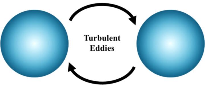
59 Figure 2-2: Schematics of one-group interfacial area transport equation source/sink mechanisms. 43

60 44 In view of these mechanisms and the general one-group interfacial area transport equation given by Equation [1-21], the one-dimensional, one-group interfacial area transport equation applicable to adiabatic, vertical, air-water bubbly flow that was implemented to establish the pilot code TRACE-T1 (Kim and Talley, 2009; Kim et al., 2011) is given as: + = [2-55] Note that in Equation [2-55] it is assumed that the interfacial area concentration weighted interfacial velocity is approximated as (Kim, 1999): [2-56] Thus, the velocity in the interfacial area transport equation is obtained from the solution of the equations of motion in TRACE-T1. It is also assumed that the average of a product is equal to the product of the averages of two variables such that the covariance terms are neglected in the averaging process; this assumption is also made in the development of the other field equations in TRACE (TRACE v5.0 Theory Manual, 2007). Note that since the one-group interfacial area transport equation regards the dispersed phase as a single group, the group subscript (i.e. 1 or 2) is omitted from the variables. Therefore, and in the present context refer to the single dispersed gas field void fraction and velocity, respectively, as opposed to the continuous gas field parameters presented in Section 2.2. To simplify the notation, the averaging operators are dropped in the remainder of this discussion, and all parameters are regarded as average values. Thus, the interfacial area concentration source/sink terms in Equation [2-55] are given as (Wu et al., 1998; Kim, 1999): = [2-57]

61 1 = 18 1 exp > [2-58] 45 1 = 3 1 exp [2-59] 1 = 3 [2-60] Here, represents the interfacial area concentration source/sink due to expansion/contraction of the bubbles, which is mainly a function of the pressure gradient for adiabatic flows. The terms,, and are the interfacial area concentration source due to turbulence impact breakup, sink due to random collision coalescence, and sink due to wake entrainment coalescence, respectively. The interfacial area source due to phase change,, is neglected since the development of TRACE-T1 focused on adiabatic flows.,,, and are empirical coefficients. Physically, these coefficients capture stochastic effects of bubble interaction phenomena that would be difficult to characterize analytically. The values of the mechanism coefficients employed in TRACE-T1 are provided in Table 2-1 for vertical co-current upward and downward air-water two-phase flows in round pipes. Table 2-1: One-group IATE model coefficients implemented into TRACE-T1 for vertical upward and vertical co-current downward flow configurations in round pipes. Mechanisms Vertical Upward (Ishii et al., 2002a) Vertical Co-current Downward (Ishii et al., 2004) TI (Source) ( = 6) ( = 6) RC (Sink) (=3; = 0.75) (=3; = 0.75) WE (Sink)

62 46 In Equation [2-59], denotes the void fraction at the maximum-packing limit, which was determined by assuming a hexagonal close-packed bubble arrangement (Kim, 1999). In order for the turbulence breakup mechanism, Equation [2-58], to activate, the flow must have a Weber number greater than the critical value,. This threshold corresponds to the point where the turbulence in the liquid is sufficient to overcome the surface tension of the bubble and cause disintegration (Kim, 1999). The Weber number is given by: = [2-61] Both TRACE v5.0 and TRACE-T1 require the surface tension,, to estimate the interfacial area concentration. TRACE v5.0 requires the surface tension to estimate the bubble diameter through Equation [2-12], and TRACE-T1 uses the surface tension to compute the Weber number in the turbulence impact breakup mechanism. Thus, an incorrect surface tension can cause the turbulence impact source term to activate non-physically, which in turn affects the estimation of the interfacial area concentration in TRACE-T1. While, TRACE is primarily a steam-water code, calculations of air-water systems are possible. However, it was found that the surface tension estimate through a steam-water correlation using the saturation temperature did not yield the correct value when evaluating airwater experimental data at room temperature. In view of the importance of the surface tension in both the conventional and transport approaches to specifying the interfacial area concentration, the steam-water correlation was revised to be evaluated at room temperature, which yielded the correct value for the air-water systems near ambient conditions. In order to reflect this change in calculations using the conventional approach, a separate code version, TRACE-NT, where NT implies non-transport, was created from the TRACE-T1 framework. TRACE-NT functions in the same manner as TRACE v5.0 in regards to a two-field, two-fluid model approach to gas-liquid

63 47 two-phase flow with the same algebraic relations to specify the interfacial area concentration (Kim et al. 2011). In Equations [2-58], [2-59], and [2-61], is the turbulent fluctuation velocity. In the development of the models (Wu et al., 1998; Kim, 1999), it was assumed that the turbulence is both isotropic and homogenous, such that is given as (Batchelor, 1951; Rotta, 1972): = / [2-62] Where the turbulent energy dissipation rate,, is given as: = 2 [2-63] Here, the two-phase friction factor,, and mixture velocity,, are specified as: = [2-64] = + (1 ) + (1 ) [2-65] Where the mixture Reynolds number,, and mixture viscosity,, are calculated as: = [2-66]

64 48 = 1 [2-67] The mixture viscosity accounts for the increased apparent viscosity of the mixture due to the presence of bubbles (Ishii and Chawla, 1979). The wake entrainment mechanism given by Equation [2-60] accounts for coalescence due to acceleration of bubbles in the wake region of leading bubbles. Thus, this mechanism is a function of the bubble drag characteristics. The bubble drag coefficient,, in Equation [2-60] is calculated from the correlation given by Ishii and Chawla (1979) for the viscous drag regime: = [2-68] Where the bubble Reynolds number is computed as: = [2-69] The relative velocity between the gas and liquid,, in Equation [2-60] could be obtained from the equations of motion in TRACE. However, to be consistent with the original development of the model and an independent calculation of the one-group interfacial area transport equation in MATLAB that was used for verification of the TRACE-T1 implementation, the relative velocity is calculated iteratively using Equations [2-68] and [2-69] and the following expression: = 4 Δ(1 ) 3 [2-70]

65 49 Here, Δ indicates the difference between the dispersed and continuous phase densities. Equation [2-70] can be obtained by considering the steady-state, one-dimensional momentum equations in the two-fluid model (Ishii and Chawla, 1979) TRACE-T1 Input The major difference between the conventional TRACE (i.e. TRACE-NT or TRACE v5.0) input deck and the TRACE-T1 input deck is how the FILL component is utilized. The FILL component is used to provide inlet flow conditions to the PIPE component in TRACE. In conventional TRACE, the system model for a vertical round pipe two-phase flow problem is shown in Figure 2-3(a). Here, a single FILL specifies all of the inlet boundary conditions, including: pressure (), liquid temperature ( ), gas temperature ( ), liquid velocity ( ), gas velocity ( ), and void fraction (). However, as can be seen in Figure 2-3(b), TRACE-T1 employs two FILLs: one for the continuous liquid and continuous gas and another for the dispersed gas field. The second FILL for the dispersed gas field is connected as a side junction to the first volume of the PIPE. Although the dispersed phase FILL is shown as a side junction with a junction angle of θ = 90, this angle is set to θ = 0 in the input deck to avoid junction models (such as a TEE junction), which can cause a sudden change in the downstream pressure solution. As noted earlier, the inputs to the continuous gas field are taken to be zero, and as such, the FILL connected to the inlet face of the pipe is used to specify only inlet liquid properties (,, and ) in TRACE-T1. The FILL connected to the side junction of the PIPE volume specifies the one-group dispersed field inlet properties (,,,, and ). Note that unlike the conventional versions of TRACE, the TRACE-T1 input deck requires a boundary condition on the interfacial area concentration since it is specified through a transport equation.

66 50 (a) (b) Figure 2-3: Pipe models for (a) TRACE-NT and (b) TRACE-T1. Since the dispersed gas FILL is connected as a side junction to the first computational volume of the PIPE, the volume immediately downstream is regarded as a mixing volume in order to isolate any effects that the FILLs might have on the solution in the PIPE. Therefore, when making predictions of experimental data to assess TRACE-T1, which will be discussed in Chapter 3, a volume downstream of the mixing volume is taken to be the location of the first axial measurement point. For consistency, the same PIPE nodalization is employed for the solutions obtained with TRACE-NT and TRACE-T1 in the assessment. Since a PIPE volume

67 51 beyond the FILL is considered as the location of the first measurement point, the values specified in the FILL are different from the experimental values. Thus, some iteration of the FILL and BREAK parameters is required to provide the correct inlet boundary conditions in TRACE-T1 and TRACE-NT. In TRACE, the BREAK component is used to specify the exit conditions of the PIPE. The break pressure governs the overall pressure in the PIPE, so iteration of the BREAK pressure is needed in order to match the inlet pressure boundary condition. Thus, the BREAK pressure is iterated upon until the pressure in the PIPE cell corresponding to the location of the first measurement port matches the reported value. During the iteration on the BREAK pressure in TRACE-T1, the FILL values for the dispersed phase void fraction, gas velocity, and interfacial area concentration are set as the experimental values obtained at the first measurement location. Once the pressure field is matched, iteration continues for the dispersed void fraction and interfacial area concentration by varying their values in the FILL. A similar iteration process is performed with TRACE-NT. However, since the interfacial area concentration is calculated with an algebraic relation internal to the code, only the void fraction is varied in the FILL for runs with TRACE-NT. Although the liquid and gas velocities are input in the FILL(s) for both TRACE-NT and TRACE-T1, iteration on these parameters cannot be performed because TRACE calculates the downstream velocities in the PIPE through the equation of motion. With the one-group interfacial area transport equation implemented into TRACE, it is important to consider that a critical part of model and code development is validation against experimental data. Previous studies (Ishii et al., 2002a, Kim et al., 2002; Ishii et al., 2009) have evaluated the one-group interfacial area transport equation against an extensive two-phase flow experimental database established in round pipes and a rectangular channel. In these studies, it was demonstrated that the one-group interfacial area transport equation can predict the interfacial

68 52 area concentration well, generally within ±20% of experimental data. However, the evaluation of the interfacial area transport equation in these studies was not coupled to the two-fluid model, as it is in TRACE-T1. Thus, TRACE-T1 requires a similar level of assessment in a wide range of experimental conditions to confirm that the implementation of the one-group interfacial area transport equation performs as intended within the TRACE framework. Additionally, comparisons of TRACE-T1 and TRACE-NT solutions can be used to investigate the differences between the interfacial area transport and conventional flow regime-based approaches. As such, Chapter 3 presents the experimental databases that are used to assess the codes and the major assessment results.

69 53 Chapter 3 Assessment of TRACE-T1 To assess the implementation of the one-group interfacial area transport equation in TRACE-T1, experimental databases established in various inner diameter round pipes for vertical co-current upward (2.54, 4.83, 10.16, 15.24, and cm ID) and downward (2.54 and 5.08 cm ID) air-water two-phase flows are utilized (Ishii et al., 2002b; Ishii et al., 2010a; Ishii et al., 2010b). The co-current upward 2.54 cm database was provided directly by the Institute of Thermal-Hydraulics at Purdue University for this assessment; a tabulation of the provided data is given in Kim et al. (2011). The databases contain pressure measurements obtained with a differential pressure transducer and local void fraction, bubble velocity, and interfacial area concentration data obtained with the multi-sensor conductivity probe (Kim et al., 2000) throughout the pipes cross-sections. Measurements of these parameters were acquired at three axial locations along the flow channels. Table 3-1 summarizes the databases used in the present assessment and indicates the axial distances from the channel inlet where measurements were obtained in terms of the non-dimensional length to pipe diameter ratio (L/D). Table 3-1: Summary of round pipe experimental databases and axial measurment locations. Two-Phase Flow Configuration Vertical Upward (Ishii et al., 2002b; Ishii et al., 2010a; Ishii et al., 2010b) Vertical Co-current Downward (Ishii et al., 2002b) Pipe Inner Diameter [cm] Axial Measurement Locations L/D , 65, , 30, , 20, , 18, , 10, , 68, , 34, 67

70 54 A total of 50 flow conditions from the databases are chosen to cover a wide extent of the bubbly flow regime. Considerations are made to select reliable data based on comparisons of the volumetric gas flux obtained from conductivity probe measurements (i.e. ) and the same quantity obtained from measurements of the gas flow rate and pressure (i.e. ). These two parameters should be equal for a given axial location. Thus, the comparison of and provides a metric for the reliability of the data. Only conditions that benchmark within approximately ±10% are chosen for the assessment of TRACE-T1. Furthermore, only conditions that contain less than a 10% contribution to the total interfacial area concentration from group-2 bubbles are selected for assessment with the one-group code (Kim et al., 2011). Figure 3-1 shows the vertical co-current upward flow conditions used in the assessment; the bubbly-slug transition line given by Mishima and Ishii (1984) is shown as a reference. The vertical co-current downward flow conditions in pipes with inner diameters of 2.54 and 5.08 cm are shown in Figures 3-2 and 3-3, respectively. The flow regime boundaries in these Figures were determined through a self-organizing neural network technique (Ishii et al., 2004). 10 Bubbly Flow 1 j f [m/s] Slug Flow 0.1 Mishima & Ishii (1984) 2.54 cm ID 4.83 cm ID cm ID cm ID cm ID j g [m/s] Figure 3-1: Vertical co-current upward air-water two-phase flow assessment conditions in various inner diameter round pipes (Ishii et al., 2002b; Ishii et al., 2010a; Ishii et al., 2010b).

71 j g [m/s] A C-T S B -j f [m/s] A: Annular B: Bubbly C-T: Churn-Turbulent S: Slug 10 Figure 3-2: Vertical co-current downward air-water two-phase flow assessment conditions in a 2.54 cm inner diameter round pipe (Ishii et al., 2002b) j g [m/s] A Kinematic Shock C-T S Falling Film B 1 -j f [m/s] A: Annular B: Bubbly C-T: Churn-Turbulent S: Slug 10 Figure 3-3: Vertical co-current downward air-water two-phase flow assessment conditions in a 5.08 cm inner diameter round pipe (Ishii et al., 2002b).

72 56 Predictions of the area-averaged local data available from the databases are generated with TRACE-T1 and TRACE-NT to investigate any differences in the solutions obtained using the interfacial area transport equation and the conventional relations for the interfacial area concentration. This includes predictions of area-averaged void fraction, void-weighted areaaveraged bubble velocity, area-averaged interfacial area concentration as well as global pressure obtained at each axial location. In presenting the code predictions, the following nomenclature is used to distinguish amongst the various databases. The flow conditions in the vertical co-current upward databases are denoted as Run x-y, where x and y indicate the nominal pipe diameter in inches and the run number, respectively. Likewise, the flow conditions in the vertical co-current downward databases are denoted as Run xd-y, where d indicates downward. Predictions demonstrating the major results of the assessment are presented in the following sections. The full set of assessment results is given in Kim et al. (2011). 3.1 Pressure Predictions Calculation of the pressure is of central interest in thermal-hydraulic system analysis from both a safety and operational standpoint. Practical analyses require information about the pressure in a system to determine required pumping power and design for appropriate structural integrity of various components. The pressure influences the development of the void fraction, which in turn affects the evolution of the interfacial structure. This is clearly shown by the functional dependence of the bubble interaction models in the interfacial area transport equation on the void fraction. To assess the pressure predictions by TRACE-NT and TRACE-T1, only the calculated values at the second and third measurement locations are considered, since iteration on the BREAK pressure is used to specify the measured value of the pressure at the location corresponding to the first measurement port in the PIPE.

73 57 Characteristic pressure predictions are shown in Figures 3-4 and 3-5 for vertical cocurrent upward and downward flows, respectively. For the vertical upward conditions, the pressure decreases linearly along the flow due to the reduction in the hydrostatic head and frictional losses. For the vertical co-current downward conditions, the pressure increases linearly along the flow due to the increase in the hydrostatic head. As can be seen in the Figures, the TRACE-T1 and TRACE-NT predictions are nearly identical and agree well with the experimental data. This behavior is observed in general for all flow conditions considered in the assessment, and it is found that the average deviations between the predictions and the experimental data are ±0.9% and ±1.1% for TRACE-T1 and TRACE-NT, respectively. 1.75E E+05 TRACE-T1 TRACE-NT Experimental Data P [Pa] 1.35E E E E L/D [-] Figure 3-4: Characteristic pressure predictions for vertical co-current upward flow; Run 4-4 (j g = m/s and j f = m/s). ±5% error bars shown.

74 E E+05 TRACE-T1 TRACE-NT Experimental Data P [Pa] 1.35E E E E L/D [-] Figure 3-5: Characteristic pressure predictions for vertical co-current downward flow; Run 1d-4 (j g = m/s and j f = m/s). ±5% error bars shown. For adiabatic bubbly flows, the interfacial area concentration should not influence the prediction of the pressure in TRACE-NT, as it is only involved in the calculation of the mass generation rate. In TRACE-T1, however, there is an additional coupling to the interfacial area concentration through the interfacial drag. The strong agreement between the pressure predictions made by TRACE-T1 and TRACE-NT indicates that the effect of the different interfacial drag model in TRACE-T1 has a minimal effect on the pressure estimation in adiabatic air-water bubbly flows. This may be due to the large density difference between the gas and liquid phases considered. The inertia of water is much greater than that of air, so its flow governs the pressure drop in the system along with the hydrostatic head. As the density difference between the two working fluids decreases or the speed and/or amount of the gas increases, the effects of the interfacial drag may become more important.

75 Void Fraction Predictions As discussed in Section 3.1, the evolution of the void fraction plays a critical role in the development of the interfacial area concentration. The void fraction describes the amount of gas in the flow, while the interfacial area concentration provides information about its configuration. Together, these two parameters provide a fundamental geometric description of two-phase flow. Since iteration on the inlet void fraction in the FILL component is performed to specify the experimental void fraction at the location corresponding to the first measurement port in the PIPE, only predictions of the void fraction at the two downstream locations are compared to the measured void fraction data. Characteristic void fraction predictions for both flow directions are shown in Figures 3-6 and 3-7. As can be seen in the Figures, the predictions made by TRACE-T1 and TRACE-NT generally agree well with the experimental data. It is also observed that there are only small differences between the void fraction predictions made by TRACE-T1 and TRACE-NT in all of the assessed conditions, as well. The differences that do arise may be due to the differences in the interfacial drag relations, which lead to different predictions in bubble velocity. For adiabatic conditions, only hydrodynamic effects influence the void fraction, as there is no mass generation or expansion due to heating. For heated conditions, however, the influence of the different methods used to calculate the interfacial area concentration in TRACE-T1 and TRACE-NT may be more apparent since the mass generation rate given by Equation [2-7] will be affected. It is found for the conditions considered in the assessment that the average deviation of the TRACE- T1 predictions from the experimental data is ±11.6%. Likewise, the average deviation between TRACE-NT and the experimental data is found to be ±12.1%. Therefore, both codes are found to predict the void fraction equally well for adiabatic, dispersed bubbly flows.

76 TRACE-T1 TRACE-NT Experimental Data <α> [-] L/D [-] Figure 3-6: Void fraction predictions for Run 8-2 (j g = m/s and j f = m/s). ±10% error bars shown TRACE-T1 TRACE-NT Experimental Data <α> [-] L/D [-] Figure 3-7: Void fraction predictions for Run 1d-5 (j g = m/s and j f = m/s). ±10% error bars shown.

77 Gas Velocity Predictions TRACE determines the phase velocities from the equations of motion and their closure models accounting for the wall shear, interfacial shear, and momentum exchange due to mass generation. As in TRACE v5.0, TRACE-T1 and TRACE-NT set the wall shear on the gas phase to zero for the range of conditions investigated. Furthermore, since only adiabatic flows are considered, no momentum exchange occurs due to mass generation. Therefore, the only difference is the interfacial drag model used in the transport and non-transport versions of the code. In TRACE-T1, the interfacial drag coefficient is given by Equation [2-50], which depends on the bubble drag coefficient given by Equation [2-51]. Both of these equations are functions of the interfacial area concentration through the Sauter-mean diameter. Therefore, the equations of motion are coupled to the interfacial area transport equation through the interfacial drag in TRACE-T1. However, in TRACE-NT, the interfacial drag coefficient is given by Equation [2-30], which relies on the drift-velocity. The multi-sensor conductivity probe technique measures the local interfacial velocity (Kim et al., 2000). Therefore, an assumption is required that the void-weighted bubble velocity obtained from the local conductivity probe measurements is comparable to the void-weighted gas velocity predicted by TRACE. For bubbly flow where the interface does not distort significantly, this approximation is likely valid. It is noted that neither the local nor void-weighted bubble velocity information obtained with the conductivity probe was available for the 2.54 cm vertical co-current upward experiment. Therefore, this database is not included in assessing the code predictions of void-weighted bubble velocity. Unlike pressure and void fraction, iterating the inlet gas velocity in the FILL does not allow for specification of the experimental bubble velocity at the location of the first measurement port in the PIPE because it is determined by the equation of motion for the gas

78 62 phase. Therefore, the experimental velocities at the first measurement port are provided in the FILL without iteration, and the velocity predictions at the locations of all three measurement ports in the PIPE component are compared against the experimental data for the assessment. It is found that while the difference in the interfacial drag relation has little impact on the pressure drop or void fraction predictions by each code, a noticeable difference can be seen in some of the bubble velocity predictions. Two distinct characteristics are observed in comparing the velocity predictions made by TRACE-NT and TRACE-T1 depending on the orientation of the flow. For the vertical co-current upward conditions, it is found that TRACE-NT tends to overestimate the experimental data and typically predicts higher velocities than TRACE-T1, as can be seen in Figure 3-8. For the 4.83 cm vertical co-current upward database, TRACE-T1 demonstrates an improved capability over TRACE-NT in predicting the bubble velocity. The average deviations for TRACE-T1 and TRACE-NT in comparison to the experimental data for this database are ±13.6% and ±20.6%, respectively. However, for the remaining vertical cocurrent upward databases, the code predictions tend to be more similar. Overall, the average deviations between the predictions and the experimental data for the vertical co-current upward databases are ±13.7% and ±14.9% for TRACE-T1 and TRACE-NT, respectively. However, the deviations between the experimental data and the velocity predictions can still be quite large, with maximum deviations for the vertical upward conditions of ±65.9% and ±70.0% for TRACE-T1 and TRACE-NT, respectively, resulting for Run 8-2. For the vertical co-current downward conditions, it is found that TRACE-NT tends to underestimate the experimental data, while TRACE-T1 demonstrates a marked improvement in predicting the experimental velocities. An example of this trend is shown in Figure 3-9. The average deviations between the predictions and the experimental data for the vertical co-current downward databases are ±12.8% and ±25.1% for TRACE-T1 and TRACE-NT, respectively.

79 TRACE-T1 TRACE-NT Experimental Data <<v g >> [m/s] L/D [-] Figure 3-8: Bubble velocity predictions for Run 2-6 (j g = m/s and j f = m/s). ±10% error bars shown TRACE-T1 TRACE-NT Experimental Data <<v g >> [m/s] L/D [-] Figure 3-9: Bubble velocity predictions for Run 1d-3 (j g = m/s and j f = m/s). ±10% error bars shown.

80 64 Considering all of the vertical upward conditions assessed, TRACE-T1 and TRACE-NT demonstrate similar agreement with the experimental data. However, TRACE-T1 shows definite improvement in the co-current downward gas-velocity predictions. This may be due to the driftflux approach used to specify the interfacial drag in TRACE-NT. The drift-velocities used to specify the interfacial drag coefficient in TRACE-NT were developed for vertical upward flows, so they may not correctly reflect the relative motion in co-current downward flows. Alternatively, the differences in the velocity predictions for both flow orientations may be due to the profile slip factor,. In TRACE-T1, the specification of the interfacial drag was not modified from that of TRACE v4.291b (Schilling, 2007). It was found after the present assessment that although the calculation of is available for the dispersed bubble field, it was set equal to unity in TRACE v4.219b (Schilling, 2007) and thus in TRACE-T1. In TRACE-NT, however, is calculated according to Equation [2-32], as the conventional two-field TRACE framework is used. Future investigation is required to determine the influence of on the gas velocity predictions. 3.4 Interfacial Area Concentration Predictions As discussed in Section 2.3.1, TRACE-T1 employs the one-group interfacial area transport equation to calculate the interfacial area concentration. To help verify the implementation of the one-group interfacial area transport equation in TRACE-T1, an independent MATLAB script is used to evaluate the transport equation. The details of the calculation procedure in the MATLAB script are discussed in Kim et al. (2011). Since the MATLAB script and TRACE-T1 employ different solution methods, some differences are expected between the interfacial area concentration predictions obtained from each code. In TRACE-NT, the interfacial area concentration is calculated using Equation [2-11], since all of the flow conditions that are considered have area-averaged void fractions less than 30%.

81 65 Because TRACE-T1 uses a transport equation as opposed to an algebraic expression to compute the interfacial area concentration, a boundary condition is required. As such, the experimental data is used to provide the interfacial area concentration at the location of the first measurement port in the PIPE, and the predicted values at the locations of the two downstream ports are compared against the data. TRACE-NT, however, utilizes an algebraic relation to calculate the interfacial area concentration as a function of the void fraction and fluid properties. Therefore, the inlet interfacial area concentration cannot be specified in TRACE-NT. Thus, the interfacial area concentration predictions at the locations of all three measurement ports in the PIPE are used to assess TRACE-NT. Figure 3-10(a) demonstrates characteristic predictions of the interfacial area concentration by TRACE-T1, TRACE-NT, and the MATLAB script. TRACE-T1 and MATLAB demonstrate strong agreement, which suggests a correct implementation of the one-group interfacial area transport equation in TRACE-T1. The TRACE-T1 and TRACE-NT predictions of the interfacial area concentration show similar growth along the pipe. However, TRACE-NT fails to capture the initial value because the bubble diameter calculated with Equation [2-12] overestimates the experimental value, which leads to a lower prediction of the interfacial area concentration. Figure 3-10(b) shows the individual contributions to the change in the interfacial area concentration along the axial direction from random collision (RC), wake entrainment (WE), turbulence impact (TI), the velocity gradient (VG), and the pressure drop (PD) calculated by the MATLAB script. The pressure effect is the dominant source of interfacial area concentration in this condition, which explains the similar trends exhibited by TRACE-T1 and TRACE-NT. The interfacial area concentration in TRACE-NT is a linear function of the void fraction, which is primarily governed by the pressure in a steady, adiabatic flow. Therefore, in conditions where the pressure effect is dominant, TRACE-T1 and TRACE-NT can predict similar trends.

82 TRACE-T1 TRACE-NT MatLab Experimental Data <a i > [1/m] L/D [-] (a) Data RC WE VG Model TI PD Δ<a i > [1/m] L/D [-] (b) Figure 3-10: (a) Interfacial area concentration predictions made by TRACE-T1, TRACE-NT, and MATLAB for a pressure dominated condition, Run 2-4 (j g = m/s and j f = m/s). (b) Source/sink contributions from the MATLAB script. ±10% error bars shown.

83 67 In view of the results in Figure 3-10(a), one may argue that simply modifying the estimate of the average bubble diameter in TRACE-NT would yield the same prediction of the interfacial area concentration as TRACE-T1. However, the average bubble diameter depends on the flow condition, so a simple relationship like Equation [2-12] would not be able to specify the bubble diameter in general. Furthermore, while a simple geometric relationship, such as Equation [2-11], can account for the pressure effect on the development of the interfacial area concentration, it cannot fully capture the evolution of the interfacial structure because it cannot account for particle interactions. The effects of bubble coalescence and breakup interactions can be seen in the nonlinear development of interfacial area concentration shown in Figure 3-11(a). The linear trend demonstrated by TRACE-NT reflects the lack of modeling bubble interactions. For the vertical upward flows considered in this study, TRACE-NT can only predict a linear increase in the interfacial area concentration since it is essentially proportional to the pressure drop along the channel. However, TRACE-T1 can account for nonlinear effects through mechanistic models for bubble interactions. This is highlighted in Figure 3-11(b), where it is seen that turbulence impact breakup becomes a significant source of interfacial area concentration as the flow develops. Random collision coalescence is also observed to be an active sink to the interfacial area concentration, and the velocity gradient (i.e. advection) also acts to decrease the interfacial area concentration along the pipe. The total change in the interfacial area concentration becomes the summation of the sources and sinks. It is noted, that the pressure effect is still the dominant source of interfacial area concentration in this condition so that a strong nonlinear trend is not observed. However, the source due to turbulence impact breakup in addition to the pressure effect allows TRACE-T1 to capture the measured value of interfacial area concentration at the last measurement location. This would not be predicted as well if only the pressure effect on the interfacial area concentration was taken into account.

84 TRACE-T1 TRACE-NT MatLab Experimental Data <a i > [1/m] L/D [-] (a) Δ<a i > [1/m] Data RC WE VG Model TI PD L/D [-] (b) Figure 3-11: (a) Interfacial area concentration predictions made by TRACE-T1, TRACE-NT, and MATLAB demonstrating nonlinear development, Run 1-11 (j g = m/s and j f = m/s). (b) Source/sink contributions from the MATLAB script. ±10% error bars shown.

85 69 Since the development of the interfacial area concentration predicted by TRACE-NT is mainly governed by the pressure effect for the flow conditions considered in this work, it is found that TRACE-NT always predicts a linear increase in the interfacial area concentration for vertical upward flows and a linear decrease for vertical co-current downward flows. While many of the experimental conditions exhibit these trends, several conditions are identified where the trend predicted by TRACE-NT is the opposite of that observed in the experimental data. For example, the data shown in Figure 3-12(a) from the vertical-upward cm database demonstrate a decrease in interfacial area concentration along the channel. This condition exists near the bubbly-slug transition boundary, so the formation of larger bubbles due to coalescence leads to a decrease in the interfacial area concentration. TRACE-NT predicts an increase in the interfacial area concentration due to the decreasing pressure in upward flow. However, TRACE-T1 is able to capture the decreasing trend in the experimental data. Considering the contributions from the individual source/sink mechanisms in the interfacial area transport equation shown in Figure 3-12(b) for this flow condition, it is observed that the random collision coalescence sink to the interfacial area concentration is the dominant mechanism. The wake entrainment coalescence mechanism is observed to be active as well, and the velocity gradient also acts as a sink to the interfacial area concentration along the channel. The net contribution of these sinks offsets the expansion source due to the pressure drop in this vertical upward flow. This enables TRACE-T1 to predict the decreasing trend in the interfacial area concentration along the channel. TRACE-NT cannot capture this phenomenon since it does not account for the effects of bubble interactions in determining the interfacial area concentration. It can only predict trends similar to the void fraction, which is always increasing in vertical upward adiabatic flow in the absence of large acceleration.

86 TRACE-T1 TRACE-NT MatLab Experimental Data <a i > [1/m] L/D [-] (a) Δ<a i > [1/m] Data RC WE VG Model TI PD L/D [-] (b) Figure 3-12: (a) Opposing trends in TRACE-T1 and TRACE-NT predictions for decreasing interfacial area concentration in vertical-upward flow, Run 8-2 (j g = m/s and j f = m/s). (b) Source/sink contributions from the MATLAB script showing random collision coalescence as the dominant mechanism. ±10% error bars shown.

87 71 Another example of opposing trends in the predictions from TRACE-NT and TRACE-T1 is shown in Figure 3-13(a). Here, for vertical co-current downward flow, the experimental data demonstrate a significant increase along the flow channel. This growth in interfacial area concentration is counterintuitive, since the increase in pressure along the flow should lead to contraction of the bubbles, a sink to the interfacial area concentration. This behavior is seen for several of the vertical co-current downward flow conditions studied with high superficial liquid velocity, where a high level of turbulence exists. Coincidentally, TRACE-NT is able to predict the interfacial area concentration at the first measurement port for the condition shown in Figure 3-13(a). Nevertheless, TRACE-NT directly reflects its dependence on the increasing pressure by predicting a decrease in interfacial area concentration along the channel. However, in view of Figure 3-13(b), TRACE-T1 is able to predict the increase in interfacial area concentration by accounting for turbulence impact breakup. The turbulence impact breakup mechanism dominates over the pressure contraction and random collision coalescence sinks, yielding an increase in the interfacial area concentration along the flow. Overall, it found that through the use of the one-group interfacial area transport equation, TRACE-T1 demonstrates a significant improvement in predicting the interfacial area concentration compared to the conventional approach. Based on the 50 flow conditions that are assessed, the absolute percent differences from the experimental data for TRACE-NT and TRACE-T1 are ±43.6% and ±13.0%, respectively. It is noted that some of the improved agreement shown by TRACE-T1 is due to applying the experimental data from the first measurement port as a boundary condition. However, for conditions where the effects of bubble interaction mechanisms dominate over the pressure effect, such as those shown in Figures 3-12(a) and 3-13(a), the benefit of the transport approach is clearly demonstrated. The accurate prediction of these experimental conditions is only possible by accounting for the effects of the bubble interaction mechanisms.

88 TRACE-T1 TRACE-NT MATLAB Experimental Data <a i > [1/m] L/D [-] (a) Data RC WE VG Model TI PD Δ<a i > [1/m] L/D [-] (b) Figure 3-13: (a) Opposing TRACE-T1 and TRACE-NT predictions for increasing interfacial area concentration in vertical co-current downward flow, Run 1d-5 (j g = m/s and j f = m/s). (b) Source/sink contributions from the MATLAB script showing turbulence impact breakup as the dominant mechanism. ±10% error bars shown.

89 73 The development and assessment of TRACE-T1 demonstrated the feasibility and improved capability of predicting the interfacial area concentration in TRACE with the one-group interfacial area transport equation. However, the range of applicability of TRACE-T1 is limited to adiabatic, dispersed bubbly flows. As discussed in Section 1.3.3, a multi-group approach is required to treat more general two-phase flow conditions. As group-1 bubbles coalesce to form larger cap and slug bubbles, the assumption of one group of bubbles with similar sizes, shapes, and interaction behavior begins to break down. Furthermore, besides having different interfacial area, group-2 bubbles alter the flow structure and thus influence the interactions of the surrounding group-1 bubbles. Therefore, the next step in the systematic implementation of the interfacial area transport equation in TRACE is the development of an adiabatic two-group interfacial area transport pilot code.

90 74 Chapter 4 Development of a Two-Group Interfacial Area Transport Pilot Code The development of a two-group interfacial area transport pilot TRACE code is presented in this Chapter. Before discussing the selected two-group interfacial area transport model and its implementation, an overview of the major two-group source/sink mechanisms that have been identified (Ishii et al., 2002a) is provided. 4.1 Summary of Two-Group Source/Sink Mechanisms The presence of two characteristic groups of bubbles, namely small spherical/distorted group-1 bubbles and larger cap/slug/churn-turbulent group-2 bubbles, leads to both intra- and intergroup bubble interactions. Interactions where the parent and daughter particles reside within a single group are classified as intragroup interactions, whereas interactions where the parent and daughter particles reside in different groups are classified as intergroup interactions. Clearly, additional combinations of interactions can exist for flow conditions with two distinct groups of bubbles in comparison to one-group flow conditions. This leads to additional terms in the interfacial area transport equation and requires the ability to track the mass or void transfer between each bubble group through either group continuity or void transport equations. To distinguish amongst the possible interactions, the nomenclature that is depicted in Figure 4-1 is adopted to represent the source/sink terms. For a general term, a superscript in parentheses is used to indicate the interacting and resultant group(s), while a subscript is used to indicate the bubble interaction mechanism and the group affected by the interaction. For example, the superscript (11,2) indicates an intergroup interaction between two group-1 bubbles yielding a group-2 bubble, and the subscript 2,WE indicates that the term applies to group-2

91 and that the interaction mechanism is wake entrainment. For the intergroup interactions, it is important to note that the change in interfacial area concentration for one group is not the same for the other group due to different bubble shapes in each group. Thus, for a given intergroup interaction, say random collision between two group-1 bubbles to yield a group-2 bubble, separate terms are required to express the change in interfacial area concentration for each group, (,) (,) namely, for the change in group-1 and, for the change in group General Term (), Interacting groups and parent/daughter relationship (e.g. a = 11,2) Affected group (e.g. b = 2) Bubble interaction mechanism (e.g. c = WE) Figure 4-1: Two-group source/sink term nomenclature. For intragroup interactions, a shorthand version of the general notation is used since the parent and daughter particles reside within the same group. A single superscript number in parentheses is used to indicate the group in which the interaction is taking place, and a subscript indicating only the interaction mechanism is used. For example, the general superscript (2,22) indicating an intragroup interaction of a group-2 bubble yielding two group-2 bubbles is written more simply as (2). The nature of the interaction (i.e. breakup or coalescence) is then inferred from the interaction mechanism indicated in the subscript. Table 4-1 summarizes the possible interfacial area concentration source/sink mechanisms in the adiabatic two-group interfacial area transport equation that have been identified (Ishii et al.,

92 2002a). Schematics of these mechanisms are shown in Figures 4-2 through 4-7. While the expansion/contraction mechanisms do not constitute interactions between bubbles, they are included in the Table for completeness. The expansion/contraction mechanisms in adiabatic flows represent the growth of bubbles due to hydrodynamic effects. The intragroup expansion terms, () () and, are similar to those in the one-group interfacial area transport equation in that they represent bubble growth within each group. By partitioning the bubbles into two groups, the possibility of expansion/contraction across the group boundary exists, which is accounted for by (:) the intergroup expansion/contraction term,. The superscript (1:2) on this term indicates that the transfer due to expansion/contraction across the group boundary can occur from group-1 to group-2 (expansion) or from group-2 to group-1 (contraction). The remaining terms in Table 4-1 represent the major bubble interaction mechanisms, which are categorized as: random collision coalescence (RC), wake entrainment coalescence (WE), turbulence impact breakup (TI), surface instability breakup (SI), and shearing-off (SO) (Ishii et al., 2002a). The first three mechanisms are similar in principle to those characterized for 76 one-group flows. Intragroup random collision, wake entrainment, and turbulence impact interactions can occur within both group-1 and group-2. However, the possibility of intergroup interactions due to these mechanisms also arises with two groups of bubbles. The coalescence of smaller bubbles to form cap bubbles has been identified as the mechanism behind the transition from bubbly to slug flow (Mishima and Ishii, 1984). Therefore, accurate modeling of coalescence phenomena is critical to the dynamic prediction of this flow regime transition. The coalescence of group-1 bubbles to form group-2 bubbles by random collision and wake entrainment is responsible for the generation of group-2 from a purely one-group condition. Furthermore, the coalescence of group-1 bubbles and group-2 bubbles to form larger group-2 bubbles drives the evolution of the flow towards a predominately group-2 condition. Conversely,

93 the intergroup turbulence impact mechanisms, may act to counter these coalescence processes, 77 driving the flow towards a more one-group condition. The net effect of these intergroup interactions is observed in the flow regime transition from bubbly to slug flow. With the presence of group-2 bubbles in the flow, two additional interactions have been identified as major bubble interaction mechanisms, namely shearing-off of small group-1 bubbles from the rims of cap/slug bubbles and breakup of large cap bubbles due to surface instability (Ishii et al., 2002a). Group-2 bubbles can continue to grow in size due to coalescence interactions and expansion until a maximum size is reached, beyond which breakup occurs due to instability of the interface. Kataoka and Ishii (1987) cite that the maximum stable bubble limit is given as:, = 40 [4-1] For air-water systems, Equation [4-1] yields a value of approximately 11 cm. In the shearing-off mechanism, numerous small bubbles are sheared off from the rims of group-2 bubbles, leading to a significant source of group-1 bubbles, and thus interfacial area concentration.

94 78 Table 4-1: Two-group source/sink mechanisms (G1 = group-1; G2 = group-2). Mechanism Term Interaction Source/Sink () (1) (1) G1-source/G1-sink Expansion/Contraction () (2) (2) G2-source/G2-sink (:) (1) (2) (2) (1) G1-sink; G2-source G2-sink; G1-source () (1) + (1) (1) G1-sink Random Collision (RC) (,) (,), ;, (,) (,), ;, (1) + (1) (2) G1-sink; G2-source (1) + (2) (2) G1-sink; G2-source () (2) + (2) (2) G2-sink () (1) + (1) (1) G1-sink Wake Entrainment (WE) (,) (,), ;, (,) (,), ;, (1) + (1) (2) G1-sink; G2-source (1) + (2) (2) G1-sink; G2-source () (2) + (2) (2) G2-sink () (1) (1) + (1) G1-source Turbulence Impact (TI) (,) (,), ;, (,) (,), ;, (2) (1) + (1) G1-source; G2-sink (2) (2) + (1) G1-source; G2-sink Surface Instability (SI) Shearing-Off* (SO) () () (,) (,), ;, (2) (2) + (2) G2-source (2) (2) + (2) G2-source (2) (1) + (2) G1-source; G2-sink *Multiple (n) group-1 bubbles produced.

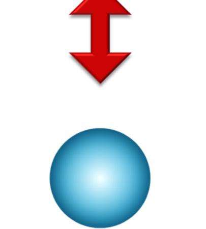
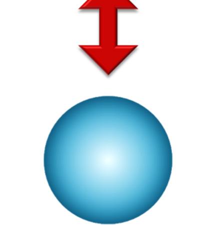
95 Figure 4-2: Schematics of intra- and intergroup bubble expansion/contraction. 79

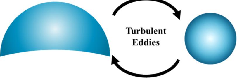
96 Figure 4-3: Schematics of intra- and intergroup random collision bubble interaction mechanisms. 80

97 Figure 4-4: Schematics of intra- and intergroup wake entrainment bubble interaction mechanisms. 81

98 Figure 4-5: Schematics of intra- and intergroup turbulence impact bubble interaction mechanisms. 82

99 83 Figure 4-6: Schematic of the surface instability bubble interaction mechanism. Figure 4-7: Schematic of the shearing-off bubble interaction mechanism.