Introduction to Econometrics. Review of Probability & Statistics

Transcription

1 1 Introduction to Econometrics Review of Probability & Statistics Peerapat Wongchaiwat, Ph.D.

2 Introduction 2 What is Econometrics? Econometrics consists of the application of mathematical statistics to economic data to lend empirical support to the models constructed by mathematical economics and to obtain numerical results. Econometrics may be defined as the quantitative analysis of actual economic phenomena based on the concurrent development of theory and observation, related by appropriate methods of inference.

3 What is Econometrics? 3 Economics Econometrics Statistics Mathematics

4 Why do we study econometrics? 4 Rare in economics (and many other areas without labs!) to have experimental data Need to use nonexperimental, or observational data to make inferences Important to be able to apply economic theory to real world data

5 Why it is so important? 5 An empirical analysis uses data to test a theory or to estimate a relationship A formal economic model can be tested Theory may be ambiguous as to the effect of some policy change can use econometrics to evaluate the program

6 The Question of Causality 6 Simply establishing a relationship between variables is rarely sufficient Want to get the effect to be considered causal If we ve truly controlled for enough other variables, then the estimated effect can often be considered to be causal

7 Purpose of Econometrics 7 Structural Analysis Policy Evaluation Economical Prediction Empirical Analysis

8 Methodology of Econometrics 8 1. Statement of theory or hypothesis. 2. Specification of the mathematical model of the theory. 3. Specification of the statistical, or econometric model. 4. Obtaining the data. 5. Estimation of the parameters of the econometric model. 6. Hypothesis testing. 7. Forecasting or prediction.

9 9 Example:Kynesian theory of consumption 1. Statement of theory or hypothesis. Keynes stated: The fundamental psychological law is that men/women are disposed, as a rule and on average, to increase their consumption as their income increases, but not as much as the increase in their income. In short, Keynes postulated that the marginal propensity to consume (MPC), the rate of change of consumption for a unit change in income, is greater than zero but less than 1

10 2.Specification of the mathematical model of the theory A mathematical economist might suggest the following form of the Keynesian consumption function: Consumption expenditure 0 1X Income

11 3. Specification of the statistical, or econometric model. To allow for the inexact relationships between economic variables, the econometrician would modify the deterministic consumption function as follows: 1 0 X u U, known as disturbance, or error term This is called an econometric model. 11

12 4. Obtaining the data. 12 year X Source: Data on (Personal Consumption Expenditure) and X (Gross Domestic Product), ) all in 1992 billions of dollars

13 13 5. Estimation of the parameters of the econometric model. reg y x Source SS df MS Number of obs = F( 1, 13) = Model Prob > F = Residual R-squared = Adj R-squared = Total Root MSE = y Coef. Std. Err. t P> t [95% Conf. Interval] x _cons

14 6. Hypothesis testing. 14 As noted earlier, Keynes expected the MPC to be positive but less than 1. In our example we found it is about Then, is 0.70 statistically less than 1? If it is, it may support Keynes s theory. Such confirmation or refutation of econometric theories on the basis of sample evidence is based on a branch of statistical theory know as statistical inference (hypothesis testing)

15 7.Forecasting or prediction. 15 To illustrate, suppose we want to predict the mean consumption expenditure for The GDP value for 1997 was billion dollars. Putting this value on the right-hand of the model, we obtain billion dollars. But the actual value of the consumption expenditure reported in 1997 was billion dollars. The estimated model thus overpredicted. The forecast error is about billion dollars.

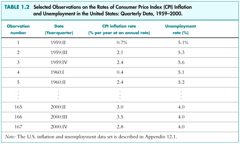
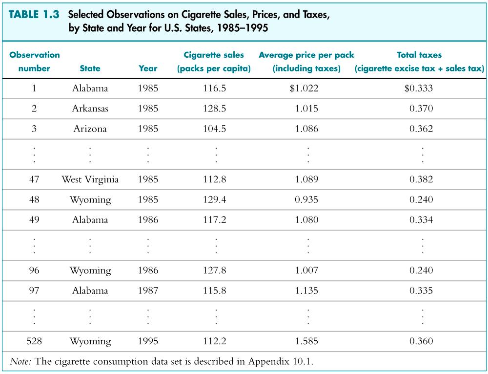
16 16 Types of Data Sets

17 17

18 18

19 19

20 Review of Probability and Statistics 20 Empirical problem: Class size and educational output Policy question: What is the effect on test scores (or some other outcome measure) of reducing class size by one student per class? By 8 students/class? We must use data to find out (is there any way to answer this without data?)

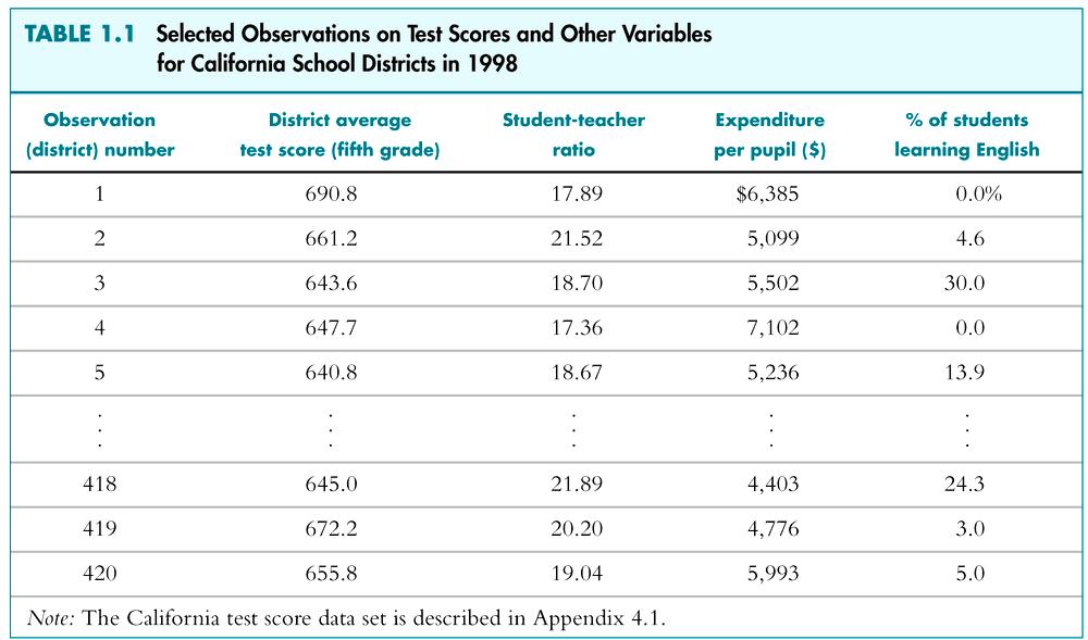
21 The California Test Score Data Set 21 All K-6 and K-8 California school districts (n = 420) Variables: 5 th grade test scores (Stanford-9 achievement test, combined math and reading), district average Student-teacher ratio (STR) = no. of students in the district divided by no. full-time equivalent teachers

22 Initial look at the data: 22 This table doesn t tell us anything about the relationship between test scores and the STR.

23 23 Question: Do districts with smaller classes have higher test scores? Scatterplot of test score v. student-teacher ratio What does this figure show?

24 24 We need to get some numerical evidence on whether districts with low STRs have higher test scores but how? 1. Compare average test scores in districts with low STRs to those with high STRs ( estimation ) 2. Test the null hypothesis that the mean test scores in the two types of districts are the same, against the alternative hypothesis that they differ ( hypothesis testing ) 3. Estimate an interval for the difference in the mean test scores, high v. low STR districts ( confidence interval )

25 Initial data analysis: Compare districts with small (STR < 20) and large (STR 20) class sizes: 25 Class Size Average score ( ) Standard deviation (sb B ) n Small Large Estimation of = difference between group means 2. Test the hypothesis that = 0 3. Construct a confidence interval for

26 1. Estimation 26 small - = large small 1 n i n small i= 1 å = = 7.4 large 1 n i å n large i= 1 Is this a large difference in a real-world sense? Standard deviation across districts = 19.1 Difference between 60 th and 75 th percentiles of test score distribution is = 8.2 This is a big enough difference to be important for school reform discussions, for parents, or for a school committee?

27 2. Hypothesis testing 27 Difference-in-means test: compute the t-statistic, t s l s l 2 2 ss sl SE( s l) n s n l where SE( s l ) is the standard error of s l, the subscripts s and l refer to small and large STR districts, and n 1 s s ( ) (etc.) 2 2 s i s ns 1 i1

28 28 Compute the difference-of-means t-statistic: Size sb B n small large t s l ss sl n s n l = 4.05 t > 1.96, so reject (at the 5% significance level) the null hypothesis that the two means are the same.

29 3. Confidence interval 29 A 95% confidence interval for the difference between the means is, ( s l ) 1.96 SE( s l ) Two equivalent statements: = = (3.8, 11.0) 1. The 95% confidence interval for doesn t include 0; 2. The hypothesis that = 0 is rejected at the 5% level.

30 What comes next 30 The mechanics of estimation, hypothesis testing, and confidence intervals should be familiar These concepts extend directly to regression and its variants Before turning to regression, however, we will review some of the underlying theory of estimation, hypothesis testing, and confidence intervals: Why do these procedures work, and why use these rather than others? So we will review the intellectual foundations of statistics and econometrics

31 Review of Statistical Theory The probability framework for statistical inference 2. Estimation 3. Testing 4. Confidence Intervals The probability framework for statistical inference (a) Population, random variable, and distribution (b) Moments of a distribution (mean, variance, standard deviation, covariance, correlation) (c) Conditional distributions and conditional means (d) Distribution of a sample of data drawn randomly from a population: 1,, n

32 (a) Population, random variable, and 32 distribution Population The group or collection of all possible entities of interest (school districts) We will think of populations as infinitely large (N is an approximation to very big ) Random variable Numerical summary of a random outcome (district average test score, district STR)

33 Population distribution of 33 The probabilities of different values of that occur in the population, for ex. Pr[ = 650] (when is discrete) or: The probabilities of sets of these values, for ex. Pr[640 < < 660] (when is continuous).

34 (b) Moments of a population distribution: mean, variance, standard deviation, covariance, correlation 34 mean = expected value (expectation) of = E() = m = long-run average value of over repeated realizations of variance = E( m ) 2 = 2 s = measure of the squared spread of the distribution standard deviation = variance = s

35 Moments, ctd. 35 skewness = 3 E 3 = measure of asymmetry of a distribution skewness = 0: distribution is symmetric skewness > (<) 0: distribution has long right (left) tail kurtosis = 4 E 4 = measure of mass in tails = measure of probability of large values kurtosis = 3: normal distribution skewness > 3: heavy tails ( leptokurtotic )

36 36

37 37 Random variables: joint distributions and covariance Random variables X and Z have a joint distribution The covariance between X and Z is cov(x,z) = E[(X m X )(Z m Z )] = s XZ The covariance is a measure of the linear association between X and Z; its units are units of X units of Z cov(x,z) > 0 means a positive relation between X and Z If X and Z are independently distributed, then cov(x,z) = 0 (but not vice versa!!) The covariance of a r.v. with itself is its variance: cov(x,x) = E[(X m X )(X m X )] = E[(X m X ) 2 ] = s 2 X

38 38 The covariance between Test Score and STR is negative: so is the correlation

39 The correlation coefficient is defined in terms of the covariance: 39 corr(x,z) = cov( X, Z) var( X) var( Z) s s s XZ = = r XZ X Z 1 < corr(x,z) < 1 corr(x,z) = 1 mean perfect positive linear association corr(x,z) = 1 means perfect negative linear association corr(x,z) = 0 means no linear association

40 40 The correlation coefficient measures linear association

41 41 (c) Conditional distributions and conditional means Conditional distributions The distribution of, given value(s) of some other random variable, X Ex: the distribution of test scores, given that STR < 20 Conditional expectations and conditional moments conditional mean = mean of conditional distribution = E( X = x) (important concept and notation) conditional variance = variance of conditional distribution Example: E(Test scores STR < 20) = the mean of test scores among districts with small class sizes The difference in means is the difference between the means of two conditional distributions:

42 Conditional mean, ctd. 42 = E(Test scores STR < 20) E(Test scores STR 20) Other examples of conditional means: Wages of all female workers ( = wages, X = gender) Mortality rate of those given an experimental treatment ( = live/die; X = treated/not treated) If E(X Z) = const, then corr(x,z) = 0 (not necessarily vice versa however) The conditional mean is a (possibly new) term for the familiar idea of the group mean

43 (d) Distribution of a sample of data drawn randomly from a population: 1,, n 43 We will assume simple random sampling Choose and individual (district, entity) at random from the population Randomness and data Prior to sample selection, the value of is random because the individual selected is random Once the individual is selected and the value of is observed, then is just a number not random The data set is ( 1, 2,, n ), where i = value of for the i th individual (district, entity) sampled

44 44 Distribution of 1,, n under simple random sampling Because individuals #1 and #2 are selected at random, the value of 1 has no information content for 2. Thus: 1 and 2 are independently distributed 1 and 2 come from the same distribution, that is, B 1, 2 are identically distributed That is, under simple random sampling, 1 and 2 are independently and identically distributed (i.i.d.). More generally, under simple random sampling, { i }, i = 1,, n, are i.i.d. This framework allows rigorous statistical inferences about moments of population distributions using a sample of data from that population

45 1. The probability framework for statistical inference 2. Estimation 3. Testing 4. Confidence Intervals Estimation is the natural estimator of the mean. But: (a) What are the properties of? (b) Why should we use rather than some other estimator? 1 (the first observation) maybe unequal weights not simple average 45 median( 1,, n ) The starting point is the sampling distribution of

46 (a) The sampling distribution of 46 is a random variable, and its properties are determined by the sampling distribution of The individuals in the sample are drawn at random. Thus the values of ( 1,, n ) are random Thus functions of ( 1,, n ), such as, are random: had a different sample been drawn, they would have taken on a different value The distribution of over different possible samples of size n is called the sampling distribution of. The mean and variance of are the mean and variance of its sampling distribution, E( ) and var( ). The concept of the sampling distribution underpins all of econometrics.

47 The sampling distribution of, ctd. 47 Example: Suppose takes on 0 or 1 (a Bernoulli random variable) with the probability distribution, Pr[ = 0] =0.22, Pr( =1) = 0.78 Then E() = p 1 + (1 p) 0 = p = 0.78 s = E[ E()] 2 = p(1 p) [remember this?] 2 = 0.78(1 0.78) = The sampling distribution of depends on n. Consider n = 2. The sampling distribution of is, Pr( = 0) = = Pr( = ½) = = Pr( = 1) = =

48 48 The sampling distribution of (p =.78): when is Bernoulli

49 49 Things we want to know about the sampling distribution: What is the mean of? If E( ) = true = 0.78, then is an unbiased estimator of What is the variance of? How does var( ) depend on n (famous 1/n formula) Does become close to when n is large? Law of large numbers: is a consistent estimator of appears bell shaped for n large is this generally true? In fact, is approximately normally distributed for n large (Central Limit Theorem)

50 The mean and variance of the sampling distribution of 50 General case that is, for i i.i.d. from any distribution, not just Bernoulli: 1 n n 1 1 n mean: E( ) = E( i ) = E ( i ) = = n n n Variance: var( ) = E[ E( )] 2 i 1 i 1 = E[ ] 2 = E 1 = E n 1 n i n i1 n i1 ( i ) 2 2 i1

51 so 1 var( ) = E n n i1 ( i ) 2 n n 1 1 = E ( i ) ( j ) n i1 n j1 1 = 2 n 1 n n i1 j1 n n = 2 n i 1 j 1 E ( i )( j ) cov(, ) i j 51 = = 1 n 2 2 i1 n 2 n

52 52 Mean and variance of sampling distribution of, ctd. E( ) = var( ) = 2 n Implications: 1. is an unbiased estimator of (that is, E( ) = ) 2. var( ) is inversely proportional to n the spread of the sampling distribution is proportional to 1/ n Thus the sampling uncertainty associated with is proportional to 1/ n (larger samples, less uncertainty, but square-root law)

53 53 The sampling distribution of is large when n For small sample sizes, the distribution of is complicated, but if n is large, the sampling distribution is simple! 1. As n increases, the distribution of becomes more tightly centered around (the Law of Large Numbers) 2. Moreover, the distribution of becomes normal (the Central Limit Theorem)

54 The Law of Large Numbers: 54 An estimator is consistent if the probability that its falls within an interval of the true population value tends to one as the sample size increases. 2 If ( 1,, n ) are i.i.d. and <, then is a consistent estimator of, that is, Pr[ < ] 1 as n which can be written, p ( p means converges in probability to ). 2 (the math: as n, var( ) = 0, which implies that Pr[ < ] 1.) n

55 55 The Central Limit Theorem (CLT): 2 If ( 1,, n ) are i.i.d. and 0 < <, then when n is large the distribution of is well approximated by a normal distribution. 2 is approximately distributed N(, ) ( normal n 2 distribution with mean and variance /n ) n ( )/ is approximately distributed N(0,1) (standard normal) E( ) That is, standardized = = is var( ) / n approximately distributed as N(0,1) The larger is n, the better is the approximation.

56 56 Sampling distribution of Bernoulli, p = 0.78: when is

57 57 E( ) Same example: sampling distribution of : var( )

58 Summary: The Sampling Distribution of 58 2 For 1,, n i.i.d. with 0 < <, The exact (finite sample) sampling distribution of has mean ( is an unbiased estimator of ) and variance 2 /n Other than its mean and variance, the exact distribution of is complicated and depends on the distribution of (the population distribution) When n is large, the sampling distribution simplifies: p (Law of large numbers) E( ) var( ) is approximately N(0,1) (CLT)

59 (b) Why Use To Estimate? 59 is unbiased: E( ) = is consistent: p is the least squares estimator of ; solves, n min ( m) m i1 i 2 so, minimizes the sum of squared residuals optional derivation n n n d 2 d ( i m) = 2 ( i m ) = 2 ( i m) dm i 1 i1 dm i1 Set derivative to zero and denote optimal value of m by ˆm: n = i1 n mˆ = i1 ˆ nm or ˆm = 1 n i i 1 n =

60 Why Use To Estimate?, ctd. 60 has a smaller variance than all other linear unbiased estimators: consider the estimator, ˆ n 1 a, where i i n i1 {a i } are such that ˆ is unbiased; then var( ) var( ˆ ) isn t the only estimator of can you think of a time you might want to use the median instead?

61 1. The probability framework for statistical inference 2. Estimation 3. Hypothesis Testing 4. Confidence intervals Hypothesis Testing The hypothesis testing problem (for the mean): make a provisional decision, based on the evidence at hand, whether a null hypothesis is true, or instead that some alternative hypothesis is true. That is, test H 0 : E() =,0 vs. H 1 : E() >,0 (1-sided, >) H 0 : E() =,0 vs. H 1 : E() <,0 (1-sided, <) H 0 : E() =,0 vs. H 1 : E(),0 (2-sided) 61

62 Some terminology for testing statistical hypotheses: p-value = probability of drawing a statistic (e.g. ) at least as 62 adverse to the null as the value actually computed with your data, assuming that the null hypothesis is true. The significance level of a test is a pre-specified probability of incorrectly rejecting the null, when the null is true. Calculating the p-value based on : p-value = Pr [ ] act H0,0,0 where act is the value of actually observed (nonrandom)

63 Calculating the p-value, ctd. 63 To compute the p-value, you need the to know the sampling distribution of, which is complicated if n is small. If n is large, you can use the normal approximation (CLT): p-value = Pr [ ], = = act H0,0,0 act,0,0 Pr H [ ] 0 / n / act,0,0 Pr H [ ] 0 n probability under left+right N(0,1) tails where = std. dev. of the distribution of = / n.

64 Calculating the p-value with known: 64 For large n, p-value = the probability that a N(0,1) random variable falls outside ( act,0 )/ In practice, is unknown it must be estimated

65 Estimator of the variance of : 65 Fact: 2 s = 1 n n 2 ( i ) 1 = sample variance of i1 If ( 1,, n ) are i.i.d. and E( 4 ) <, then 2 s p 2 Why does the law of large numbers apply? Because 2 s is a sample average; see Appendix 3.3 Technical note: we assume E( 4 ) < because here the average is not of i, but of its square; see App. 3.3

66 Computing the p-value with 2 estimated: 66 so p-value = = Pr [ ], act H0,0,0 act,0,0 Pr H [ ] 0 0 p-value = / n / (large n) s / n s / n act,0,0 Pr H [ ] 0 act Pr H [ t t ] ( estimated) n 2 probability under normal tails outside t act where t = s,0 / n (the usual t-statistic)

67 What is the link between the p-value 67 and the significance level? The significance level is prespecified. For example, if the prespecified significance level is 5%, you reject the null hypothesis if t 1.96 equivalently, you reject if p The p-value is sometimes called the marginal significance level. Often, it is better to communicate the p-value than simply whether a test rejects or not the p-value contains more information than the yes/no statement about whether the test rejects.

68 At this point, you might be wondering, What happened to the t-table and the degrees of freedom? Digression: the Student t distribution If i, i = 1,, n is i.i.d. N(, ), then the t-statistic has the Student t-distribution with n 1 degrees of freedom. 2 The critical values of the Student t-distribution is tabulated in the back of all statistics books. Remember the recipe? 1. Compute the t-statistic 2. Compute the degrees of freedom, which is n 1 3. Look up the 5% critical value 4. If the t-statistic exceeds (in absolute value) this critical value, reject the null hypothesis.

69 Comments on this recipe and the Student t-distribution The theory of the t-distribution was one of the early triumphs of mathematical statistics. It is astounding, really: if is i.i.d. normal, then you can know the exact, finite-sample distribution of the t-statistic it is the Student t. So, you can construct confidence intervals (using the Student t critical value) that have exactly the right coverage rate, no matter what the sample size. This result was really useful in times when computer was a job title, data collection was expensive, and the number of observations was perhaps a dozen. It is also a conceptually beautiful result, and the math is beautiful too which is probably why stats profs love to teach the t-distribution. But.

70 Comments on Student t distribution, ctd If the sample size is moderate (several dozen) or large (hundreds or more), the difference between the t-distribution and N(0,1) critical values are negligible. Here are some 5% critical values for 2-sided tests: degrees of freedom (n 1) 5% t-distribution critical value

71 Comments on Student t distribution, ctd So, the Student-t distribution is only relevant when the sample size is very small; but in that case, for it to be correct, you must be sure that the population distribution of is normal. In economic data, the normality assumption is rarely credible. Here are the distributions of some economic data. Do you think earnings are normally distributed? Suppose you have a sample of n = 10 observations from one of these distributions would you feel comfortable using the Student t distribution?

72 72

73 Comments on Student t distribution, ctd ou might not know this. Consider the t-statistic testing the hypothesis that two means (groups s, l) are equal: s l s l t 2 2 ss sl SE( s l) n s n l Even if the population distribution of in the two groups is normal, this statistic doesn t have a Student t distribution! There is a statistic testing this hypothesis that has a normal distribution, the pooled variance t-statistic however the pooled variance t-statistic is only valid if the variances of the normal distributions are the same in the two groups. Would you expect this to be true, say, for men s v. women s wages?

74 The Student-t distribution summary 74 The assumption that is distributed N(, ) is rarely plausible in practice (income? number of children?) For n > 30, the t-distribution and N(0,1) are very close (as n grows large, the t n 1 distribution converges to N(0,1)) The t-distribution is an artifact from days when sample sizes were small and computers were people For historical reasons, statistical software typically uses the t-distribution to compute p-values but this is irrelevant when the sample size is moderate or large. For these reasons, in this class we will focus on the large-n approximation given by the CLT 2

75 1. The probability framework for statistical inference 2. Estimation 3. Testing 4. Confidence intervals Confidence Intervals A 95% confidence interval for is an interval that contains the true value of in 95% of repeated samples. 75 Digression: What is random here? The values of 1,, n and thus any functions of them including the confidence interval. The confidence interval it will differ from one sample to the next. The population parameter,, is not random, we just don t know it.

76 Confidence intervals, ctd. 76 A 95% confidence interval can always be constructed as the set of values of not rejected by a hypothesis test with a 5% significance level. { : s / n 1.96} = { : 1.96 s = { : 1.96 sn s 1.96 n } = { ( 1.96 sn, s n )} / n 1.96} This confidence interval relies on the large-n results that is approximately normally distributed and 2 s p 2.

77 Summary: 77 From the two assumptions of: (1) simple random sampling of a population, that is, { i, i =1,,n} are i.i.d. (2) 0 < E( 4 ) < we developed, for large samples (large n): Theory of estimation (sampling distribution of ) Theory of hypothesis testing (large-n distribution of t- statistic and computation of the p-value) Theory of confidence intervals (constructed by inverting test statistic) Are assumptions (1) & (2) plausible in practice? es