Introduction to Econometrics

Transcription

1 Introduction to Econometrics STAT-S-301 Experiments and Quasi-Experiments (2016/2017) Lecturer: Yves Dominicy Teaching Assistant: Elise Petit 1

2 Why study experiments? Ideal randomized controlled experiments provide a benchmark for assessing observational studies. Actual experiments are rare ($$$) but influential. Experiments can solve the threats to internal validity of observational studies, but they have their own threats to internal validity. Thinking about experiments helps us to understand quasi-experiments, or natural experiments, in which there some variation is as if randomly assigned. 2

3 Terminology: experiments and quasi-experiments An experiment is designed and implemented consciously by human researchers. An experiment entails conscious use of a treatment and control group with random assignment (e.g. clinical trials of a drug). A quasi-experiment or natural experiment has a source of randomization that is as if randomly assigned, but this variation was not part of a conscious randomized treatment and control design. Program evaluation is the field of statistics aimed at evaluating the effect of a program or policy, for example, an ad campaign to cut smoking or a job training program. 3

4 Different types of experiments: three examples Clinical drug trial: does a proposed drug lower cholesterol? o Y = cholesterol level o X = treatment or control group (or dose of drug) Job training program (Job Training Partnership Act) o Y = has a job, or not (or Y = wage income) o X = went through experimental program, or not Class size effect (Tennessee class size experiment) o Y = test score (Stanford Achievement Test) o X = class size treatment group (regular, regular + aide, small) 4

5 Our treatment of experiments: brief outline Why (precisely) do ideal randomized controlled experiments provide estimates of causal effects? What are the main threats to the validity (internal and external) of actual experiments that is, experiments actually conducted with human subjects? Flaws in actual experiments can result in X and u being correlated (threats to internal validity). Some of these threats can be addressed using the regression estimation methods we have used so far: multiple regression, panel data, IV regression. 5

6 Idealized Experiments and Causal Effects An ideal randomized controlled experiment randomly assigns subjects to treatment and control groups. More generally, the treatment level X is randomly assigned: Y i = X i + u i. If X is randomly assigned (for example by computer) then u and X are independently distributed and E(u i X i ) = 0, so OLS yields an unbiased estimator of 1. The causal effect is the population value of 1 in an ideal randomized controlled experiment. 6

7 Estimation of causal effects in an ideal randomized controlled experiment Random assignment of X implies that E(u i X i ) = 0. ˆ Thus the OLS estimator 1 is unbiased. When the treatment is binary, ˆ 1 is just the difference in mean outcome (Y) in the treatment vs. control group ( treated Y control Y ). This differences in means is sometimes called the differences estimator. 7

8 Potential Problems with Experiments in Practice Threats to Internal Validity 1. Failure to randomize (or imperfect randomization) for example, openings in job treatment program are filled on first-come, first-serve basis; latecomers are controls, result is correlation between X and u. 2. Failure to follow treatment protocol (or partial compliance ) some controls get the treatment, some treated get controls, 8

9 errors-in-variables bias: corr(x,u) 0, Attrition (some subjects drop out), suppose the controls who get jobs move out of town; then corr(x,u) Experimental effects experimenter bias (conscious or subconscious): treatment X is associated with extra effort or extra care, so corr(x,u) 0, subject behavior might be affected by being in an experiment, so corr(x,u) 0 (Hawthorne effect). 9

10 Just as in regression analysis with observational data, threats to the internal validity of regression with experimental data implies that corr(x,u) 0 so OLS (the differences estimator) is biased. 10

11 Threats to External Validity 1. Nonrepresentative sample. 2. Nonrepresentative treatment (that is, program or policy). 3. General equilibrium effects (effect of a program can depend on its scale; admissions counseling). 4. Treatment v. eligibility effects (which is it you want to measure: effect on those who take the program, or the effect on those are eligible). 11

12 Regression Estimators of Causal Effects Using Experimental Data Focus on the case that X is binary (treatment/control). Often you observe subject characteristics, W 1i,,W ri. Extensions of the differences estimator: o can improve efficiency (reduce standard errors) o can eliminate bias that arises when: treatment and control groups differ there is conditional randomization there is partial compliance These extensions involve methods we have already seen multiple regression, panel data, IV regression. 12

13 The differences-in-differences estimator Suppose the treatment and control groups differ systematically; maybe the control group is healthier (wealthier; better educated; etc.). Then X is correlated with u, and the differences estimator is biased. The differences-in-differences estimator adjusts for preexperimental differences by subtracting off each subject s pre-experimental value of Y: o Y before i = value of Y for subject i before the expt, Y = value of Y for subject i after the expt, o after i o Y i = after Y i before Y i = change over course of expt. 13

14 ˆ 1 diffs in diffs = ( treat, after treat, before control, after control, before Y Y ) ( Y Y ) 14

15 (1) Differences formulation: Y i = X i + u i where after before Y i = Y i Y i X i = 1 if treated, = 0 otherwise ˆ 1 is the diffs-in-diffs estimator 15

16 (2) Equivalent panel data version: Y it = X it + 2 D it + 3 G it + v it, i = 1,,n where t = 1 (before experiment), 2 (after experiment) D it = 0 for t = 1, = 1 for t = 2 G it = 0 for control group, = 1 for treatment group X it = 1 if treated, = 0 otherwise = D it G it = interaction effect of being in treatment group in the second period ˆ 1 is the diffs-in-diffs estimator 16

17 Including additional subject characteristics (W s) Typically you observe additional subject characteristics, W 1i,,W ri. Differences estimator with add l regressors: Y i = X i + 2 W 1i + + r+1 W ri + u i Differences-in-differences estimator with W s: Y i = X i + 2 W 1i + + r+1 W ri + u i where Y i = after Y i before Y i. 17

18 Why include additional subject characteristics (W s)? 1. Efficiency: more precise estimator of 1 (smaller standard errors). 2. Check for randomization. If X is randomly assigned, then the OLS estimators with and without the W s. should be similar if they aren t, this suggests that X wasn t randomly designed (a problem with the expt.) Note: To check directly for randomization, regress X on the W s and do a F-test. 3. Adjust for conditional randomization (we ll return to this later ). 18

19 Estimation when there is partial compliance Consider diffs-in-diffs estimator, X = actual treatment Y i = X i + u i. Suppose there is partial compliance: some of the treated don t take the drug; some of the controls go to job training anyway. Then X is correlated with u, and OLS is biased Suppose initial assignment, Z, is random. Then (1) corr(z,x) 0 and (2) corr(z,u) = 0. Thus 1 can be estimated by TSLS, with instrumental variable Z = initial assignment. This can be extended to W s (included exog. variables). 19

20 Experimental Estimates of the Effect of Reduction: The Tennessee Class Size Experiment Project STAR (Student-Teacher Achievement Ratio) 4-year study, $12 million. Upon entering the school system, a student was randomly assigned to one of three groups: o regular class (22 25 students) o regular class + aide o small class (13 17 students). regular class students re-randomized after first year to regular or regular+aide. Y = Stanford Achievement Test scores. 20

21 Deviations from experimental design Partial compliance: o 10% of students switched treatment groups because of incompatibility and behavior problems how much of this was because of parental pressure? o Newcomers: incomplete receipt of treatment for those who move into district after grade 1. Attrition o students move out of district o students leave for private/religious schools 21

22 Regression analysis The differences regression model: Y i = SmallClass i + 2 RegAide i + u i where SmallClass i = 1 if in a small class RegAide i = 1 if in regular class with aide Additional regressors (W s) o teacher experience o free lunch eligibility o gender, race 22

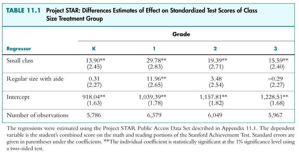
23 23

24 24

25 How big are these estimated effects? Put on same basis by dividing by std. dev. of Y. Units are now standard deviations of test scores. 25

26 How do these estimates compare to those from the California, Mass. observational studies? 26

27 What is the Difference Between a Control Variable and the Variable of Interest? Example: free lunch eligible in the STAR regressions Coefficient is large, negative, statistically significant. Policy interpretation: Making students ineligible for a free school lunch will improve their test scores. Is this really an estimate of a causal effect? Is the OLS estimator of its coefficient unbiased? Can it be that the coefficient on free lunch eligible is biased but the coefficient on SmallClass is not? 27

28 28

29 Example: free lunch eligible Coefficient on free lunch eligible is large, negative, statistically significant. Policy interpretation: Making students ineligible for a free school lunch will improve their test scores. Why (precisely) can we interpret the coefficient on SmallClass as an unbiased estimate of a causal effect, but not the coefficient on free lunch eligible? This is not an isolated example! o Other control variables we have used: gender, race, district income, state fixed effects, time fixed effects, city (or state) population, What is a control variable anyway? 29

30 Simplest case: one X, one control variable W Y i = X i + 2 W i + u i For example, W = free lunch eligible (binary) X = small class/large class (binary) Suppose random assignment of X depends on W o for example, 60% of free-lunch eligibles get small class, 40% of ineligibles get small class). o note: this wasn t the actual STAR randomization procedure this is a hypothetical example. Further suppose W is correlated with u. 30

31 Suppose: The control variable W is correlated with u. Given W = 0 (ineligible), X is randomly assigned. Given W = 1 (eligible), X is randomly assigned. Then: Given the value of W, X is randomly assigned. That is, controlling for W, X is randomly assigned. Thus, controlling for W, X is uncorrelated with u. Moreover, E(u X,W) doesn t depend on X. That is, we have conditional mean independence: E(u X,W) = E(u W). 31

32 Implications of conditional mean independence Y i = X i + 2 W i + u i Suppose E(u W) is linear in W (not restrictive could add quadratics etc.): then, E(u X,W) = E(u W) = W i (*) so E(Y i X i,w i ) = E( X i + 2 W i + u i X i,w i ) = X i + 2 W i + E(u i X i,w i ) = X i + 2 W i W i by (*) = ( ) + 1 X i + ( )W i 32

33 The conditional mean of Y given X and W is E(Y i X i,w i ) = ( ) + 1 X i + ( )W i The effect of a change in X under conditional mean independence is the desired causal effect: E(Y i X i = x+ x,w i ) E(Y i X i = x,w i ) = 1 x or E( Yi X i x x, Wi ) E( Yi X i x, Wi ) 1 = x If X is binary (treatment/control), this becomes: E( Yi X i 1, Wi ) E( Yi X i 0, Wi ) 1 = x which is the desired treatment effect. 33

34 Y i = X i + 2 W i + u i Conditional mean independence says: E(u X,W) = E(u W) which, with linearity, implies: Then: E(Y i X i,w i ) = ( ) + 1 X i + ( )W i The OLS estimator 1 is unbiased. ˆ 2 is not consistent and not meaningful. ˆ The usual inference methods (standard errors, hypothesis tests, etc.) apply to 1. ˆ 34

35 So, what is a control variable? A control variable W is a variable that results in X satisfying the conditional mean independence condition: E(u X,W) = E(u W) Upon including a control variable in the regression, X ceases to be correlated with the error term. The control variable itself can be (in general will be) correlated with the error term. The coefficient on X has a causal interpretation. The coefficient on W does not have a causal interpretation. 35

36 Example: Effect of teacher experience on test scores More on the design of Project STAR: Teachers didn t change school because of the expt. Within their normal school, teachers were randomly assigned to small/regular/reg+aide classrooms. What is the effect of X = years of teacher education? The design implies conditional mean independence: W = school binary indicator Given W (school), X is randomly assigned That is, E(u X,W) = E(u W) W is plausibly correlated with u (nonzero school fixed effects: some schools are better/richer/etc than others). 36

37 37

38 Example: teacher experience, ctd. Without school fixed effects (2), the estimated effect of an additional year of experience is 1.47 (SE =.17). Controlling for the school (3), the estimated effect of an additional year of experience is.74 (SE =.17). Direction of bias makes sense: o less experienced teachers at worse schools o years of experience picks up this school effect. OLS estimator of coefficient on years of experience is biased up without school effects; with school effects, OLS yields unbiased estimator of causal effect. School effect coefficients don t have a causal interpretation (effect of student changing schools). 38

39 Quasi-Experiments A quasi-experiment or natural experiment has a source of randomization that is as if randomly assigned, but this variation was not part of a conscious randomized treatment and control design. Two cases: (a) Treatment (X) is as if randomly assigned (OLS) (b) A variable (Z) that influences treatment (X) is as if randomly assigned (IV) 39

40 Two types of quasi-experiments (a) Treatment (X) is as if randomly assigned (perhaps conditional on some control variables W) Ex: Effect of marginal tax rates on labor supply o X = marginal tax rate (rate changes in one state, not another; state is as if randomly assigned) (b) A variable (Z) that influences treatment (X) is as if randomly assigned (IV) Effect on survival of cardiac catheterization X = cardiac catheterization; Z = differential distance to CC hospital 40

41 Econometric methods (a) Treatment (X) is as if randomly assigned (OLS) Diffs-in-diffs estimator using panel data methods: where Y it = X it + 2 D it + 3 G it + u it, i = 1,,n t = 1 (before experiment), 2 (after experiment) D it = 0 for t = 1, = 1 for t = 2 G it = 0 for control group, = 1 for treatment group X it = 1 if treated, = 0 otherwise = D it x G it = interaction effect of being in treatment group in the second period ˆ 1 is the diffs-in-diffs estimator 41

42 The panel data diffs-in-diffs estimator simplifies to the changes diffs-in-diffs estimator when T = 2 Y it = X it + 2 D it + 3 G it + u it, i = 1,,n (*) For t = 1: D i1 = 0 and X i1 = 0 (nobody treated), so Y i1 = G i1 + u i1 For t = 2: D i2 = 1 and X i2 = 1 if treated, = 0 if not, so so Y i2 = X i G i2 + u i2 Y i = Y i2 Y i1 = ( X i G i2 +u i2 ) ( G i1 +u i1 ) = 1 X i (u i1 u i2 ) (since G i1 = G i2 ) Or Y i = X i + v i, where v i = u i1 u i2 (**) 42

43 Differences-in-differences with control variables Y it = X it + 2 D it + 3 G it + 4 W 1it r W rit + u it, X it = 1 if the treatment is received, = 0 otherwise = G it x D it (= 1 for treatment group in second period) If the treatment (X) is as if randomly assigned, given W, then u is conditionally mean indep. of X: E(u X,D,G,W) = E(u D,G,W) OLS is a consistent estimator of 1, the causal effect of a change in X In general, the OLS estimators of the other coefficients do not have a causal interpretation. 43

44 (b) A variable (Z) that influences treatment (X) is as if randomly assigned (IV) Y it = X it + 2 D it + 3 G it + 4 W 1it r W rit + u it, X it = 1 if the treatment is received, = 0 otherwise = G it x D it (= 1 for treatment group in second period) Z it = variable that influences treatment but is uncorrelated with u it (given W s) TSLS: X = endogenous regressor D,G,W 1,,W r = included exogenous variables Z = instrumental variable 44

45 Potential Threats to Quasi-Experiments The threats to the internal validity of a quasiexperiment are the same as for a true experiment, with one addition. 4. Failure to randomize (imperfect randomization) Is the as if randomization really random, so that X (or Z) is uncorrelated with u? 5. Failure to follow treatment protocol & attrition 6. Experimental effects (not applicable) 7. Instrument invalidity (relevance + exogeneity) (Maybe healthier patients do live closer to CC hospitals they might have better access to care in general) 45

46 The threats to the external validity of a quasiexperiment are the same as for an observational study. 5. Nonrepresentative sample 6. Nonrepresentative treatment (that is, program or policy) Example: Cardiac catheterization The CC study has better external validity than controlled clinical trials because the CC study uses observational data based on real-world implementation of cardiac catheterization. However that study used data from the early 90 s do its findings apply to CC usage today? 46

47 Experimental and Quasi-Experiments Estimates in Heterogeneous Populations We have discussed the treatment effect But the treatment effect could vary across individuals: o Effect of job training program probably depends on education, years of education, etc. o Effect of a cholesterol-lowering drug could depend other health factors (smoking, age, diabetes, ) If this variation depends on observed variables, then this is a job for interaction variables! But what if the source of variation is unobserved? 47

48 Heterogeneity of causal effects When the causal effect (treatment effect) varies among individuals, the population is said to be heterogeneous. When there are heterogeneous causal effects that are not linked to an observed variable: What do we want to estimate? o Often, the average causal effect in the population o But there are other choices, for example the average causal effect for those who participate (effect of treatment on the treated) What do we actually estimate? o using OLS? using TSLS? 48

49 Population regression model with heterogeneous causal effects: Y i = 0 + 1i X i + u i, i = 1,,n 1i is the causal effect (treatment effect) for the i th individual in the sample For example, in the JTPA experiment, 1i could be zero if person i already has good job search skills What do we want to estimate? o effect of the program on a randomly selected person (the average causal effect ) our main focus o effect on those most (least?) benefited o effect on those who choose to go into the program? 49

50 The Average Causal Effect Y i = 0 + 1i X i + u i, i = 1,,n The average causal effect (or average treatment effect) is the mean value of 1i in the population. We can think of 1 as a random variable: it has a distribution in the population, and drawing a different person yields a different value of 1 (just like X and Y) For example, for person #34 the treatment effect is not random it is her true treatment effect but before she is selected at random from the population, her value of 1 can be thought of as randomly distributed. 50

51 Y i = 0 + 1i X i + u i, i = 1,,n The average causal effect is E( 1 ). What does OLS estimate: (a) When the conditional mean of u given X is zero? (b) Under the stronger assumption that X is randomly assigned (as in a randomized experiment)? In this case, OLS is a consistent estimator of the average causal effect. 51

52 OLS with Heterogeneous Causal Effects Y i = 0 + 1i X i + u i, i = 1,,n (a) Suppose E(u i X i ) = 0 so cov(u i,x i ) = 0. treated If X is binary (treated/untreated), 1 = Y Y estimates the causal effect among those who receive the treatment. Why? For those treated, ˆ control treated Y reflects the effect of the treatment on them. But we don t know how the untreated would have responded had they been treated! 52

53 The math: suppose X is binary and E(u i X i ) = 0. Then ˆ 1 = For the treated: For the controls: Thus: treated Y Y control E(Y i X i =1) = 0 + E( 1i X i X i =1) + E(u i X i =1) = 0 + E( 1i X i =1) E(Y i X i =0) = 0 + E( 1i X i X i =0) + E(u i X i =0) = 0 1 ˆ p E(Y i X i =1) E(Y i X i =0) = E( 1i X i =1) = average effect of the treatment on the treated 53

54 OLS with heterogeneous treatment effects: general X with E(u i X i ) = 0 ˆ s 1 = 2 s XY X = = p XY 2 X = cov( X u, X ) 0 1i i i i var( X ) cov(, X ) cov( X, X ) cov( u, X ) 0 i 1i i i i i cov( X, X ) 1i i i var( X ) i var( X ) i i (because cov(u i,x i ) = 0) If X is binary, this simplifies to the effect of treatment on the treated Without heterogeneity, 1i = 1 and ˆ p

55 In general, the treatment effects of individuals with large values of X are given the most weight (b) Now make a stronger assumption: that X is randomly assigned (experiment or quasi-experiment). Then what does OLS actually estimate? I X i is randomly assigned, it is distributed independently of 1i, so there is no difference between the population of controls and the population in the treatment group Thus the effect of treatment on the treated = the average treatment effect in the population. 55

56 The math: ˆ p 1 cov( X, X ) 1i i i var( X ) i = E 1 i = E( 1i ) cov( X, X ) var( X i ) 1i i i = E E cov( Xi, Xi) var( X i) = E 1 i 1i var( X ) i var( X i ) 56

57 IV Regression with Heterogeneous Causal Effects Suppose the treatment effect is heterogeneous and the effect of the instrument on X is heterogeneous: Y i = 0 + 1i X i + u i X i = 0 + 1i Z i + v i (equation of interest) (first stage of TSLS) In general, TSLS estimates the causal effect for those whose value of X (probability of treatment) is most influenced by the instrument. 57

58 Y i = 0 + 1i X i + u i X i = 0 + 1i Z i + v i (equation of interest) (first stage of TSLS) Intuition: Suppose 1i s were known. If for some people 1i = 0, then their predicted value of X i wouldn t depend on Z, so the IV estimator would ignore them. The IV estimator puts most of the weight on individuals for whom Z has a large influence on X. TSLS measures the treatment effect for those whose probability of treatment is most influenced by X. 58

59 The math Y i = 0 + 1i X i + u i X i = 0 + 1i Z i + v i (equation of interest) (first stage of TSLS) To simplify things, suppose: 1i and 1i are distributed independently of (u i,v i,z i ) E(u i Z i ) = 0 and E(v i Z i ) = 0 E( 1i ) 0 Then ˆ TSLS p E( 1i 1i) 1 E( ) 1i TSLS estimates the causal effect for those individuals for whom Z is most influential (those with large 1i ). 59

60 When there are heterogeneous causal effects, what TSLS estimates depend on the choice of instruments! With different instruments, TSLS estimates different weighted averages!!! Suppose you have two instruments, Z 1 and Z 2. o In general these instruments will be influential for different members of the population. o Using Z 1, TSLS will estimate the treatment effect for those people whose probability of treatment (X) is most influenced by Z 1 o The treatment effect for those most influenced by Z 1 might differ from the treatment effect for those most influenced by Z 2 60

61 When does TSLS estimate the average causal effect? Y i = 0 + 1i X i + u i (equation of interest) X i = 0 + 1i Z i + v i (first stage of TSLS) ˆ TSLS p E( 1i 1i) 1 E( ) TSLS estimates the average causal effect (that is, ˆ TSLS p 1 E( 1i )) if: o If 1i and 1i are independent 1i o If 1i = 1 (no heterogeneity in equation of interest) o If 1i = 1 (no heterogeneity in first stage equation) But in general ˆ TSLS 1 does not estimate E( 1i )! 61

62 Example: Cardiac catheterization Y i = survival time (days) for AMI patients X i = received cardiac catheterization (or not) Z i = differential distance to CC hospital Equation of interest: SurvivalDays i = 0 + 1i CardCath i + u i First stage (linear probability model): CardCath i = 0 + 1i Distance i + v i For whom does distance have the great effect on the probability of treatment? For those patients, what is their causal effect 1i? 62

63 Equation of interest: SurvivalDays i = 0 + 1i CardCath i + u i First stage (linear probability model): CardCath i = 0 + 1i Distance i + v i TSLS estimates the causal effect for those whose value of X i is most heavily influenced by Z i TSLS estimates the causal effect for those for whom distance most influences the probability of treatment What is their causal effect? ( We might as well go to the CC hospital, its not too much farther ) This is one explanation of why the TSLS estimate is smaller than the clinical trial OLS estimate. 63

64 Heterogeneous Causal Effects: Summary Heterogeneous causal effects mean that the causal (or treatment) effect varies across individuals. When these differences depend on observable variables, heterogeneous causal effects can be estimated using interactions (nothing new here). When these differences are unobserved ( 1i ) the average causal (or treatment) effect is the average value in the population, E( 1i ). When causal effects are heterogeneous, OLS and TSLS estimate. 64

65 TSLS with Heterogeneous Causal Effects TSLS estimates the causal effect for those individuals for whom Z is most influential (those with large 1i ). What TSLS estimates depends on the choice of Z!! In CC example, these were the individuals for whom the decision to drive to a CC lab was heavily influenced by the extra distance (those patients for whom the EMT was otherwise on the fence ). Thus TSLS also estimates a causal effect: the average effect of treatment on those most influenced by the instrument: o In general, this is neither the average causal effect nor the effect of treatment on the treated. 65

66 Summary: Experiments and Quasi- Experiments Experiments: Average causal effects are defined as expected values of ideal randomized controlled experiments. Actual experiments have threats to internal validity. These threats to internal validity can be addressed (in part) by: o panel methods (differences-in-differences) o multiple regression o IV (using initial assignment as an instrument). Quasi-experiments: Quasi-experiments have an as-if randomly assigned source of variation. 66

67 This as-if random variation can generate: o X i which satisfies E(u i X i ) = 0 (so estimation proceeds using OLS); or o instrumental variable(s) which satisfy E(u i Z i ) = 0 (so estimation proceeds using TSLS). Quasi-experiments also have threats to internal vaidity. Two additional subtle issues: What is a control variable? o A variable W for which X and u are uncorrelated, given the value of W (conditional mean independence: E(u i X i,w i ) = E(u i W i ). o Example: STAR & effect of teacher experience within their school, teachers were randomly assigned to regular/reg+aide/small class. 67

68 OLS provides an unbiased estimator of the causal effect, but only after controlling for school effects. What do OLS and TSLS estimate when there is unobserved heterogeneity of causal effects? In general, weighted averages of causal effects: o If X is randomly assigned, then OLS estimates the average causal effect. o If X i is not randomly assigned but E(u i X i ) = 0, OLS estimates the average effect of treatment on the treated. o If E(u i Z i ) = 0, TSLS estimates the average effect of treatment on those most influenced by Z i. 68