Chapter 7. Hypothesis Tests and Confidence Intervals in Multiple Regression

Transcription

1 Chapter 7 Hypothesis Tests and Confidence Intervals in Multiple Regression

2 Outline 1. Hypothesis tests and confidence intervals for a single coefficie. Joint hypothesis tests on multiple coefficients 3. Other types of hypotheses involving multiple coefficients 4. How to decide what variables to include in a regression model

3 3 Hypothesis Tests and Confidence Intervals for a Single Coefficient in Multiple Regression (SW Section 7.1) ˆ β E( ˆ β ) var( ˆ β ) is approximately distributed N(0,1) (CLT). Thus hypotheses on β 1 can be tested using the usual t-statistic, and confidence intervals are constructed as { ˆ β 1 ± 1.96 SE( ˆ β 1 )}. So too for β,, β k. ˆ β 1 and ˆ β are generally not independently distributed so neither are their t-statistics (more on this later).

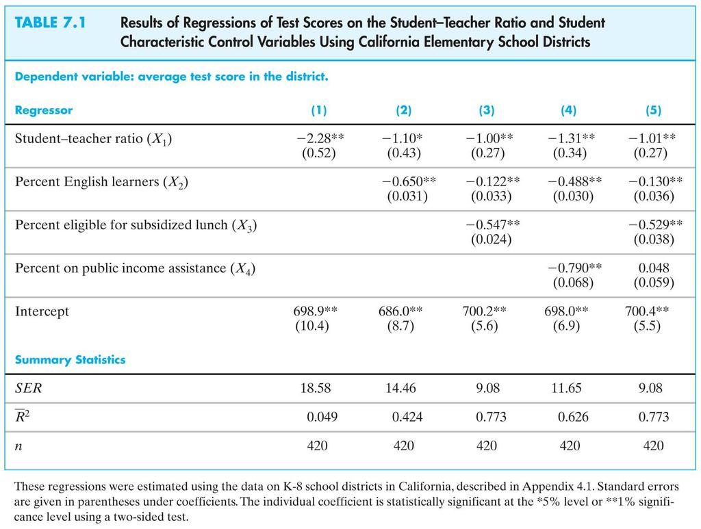
4 Example: The California class size data (1) TestScore = STR (10.4) (0.5) () TestScore = STR 0.650PctEL (8.7) (0.43) (0.031) The coefficient on STR in () is the effect on TestScores of a unit change in STR, holding constant the percentage of English Learners in the district The coefficient on STR falls by one-half The 95% confidence interval for coefficient on STR in () is { 1.10 ± } = ( 1.95, 0.6) The t-statistic testing β STR = 0 is t = 1.10/0.43 =.54, so we reject the hypothesis at the 5% significance level 4

5 Standard errors in multiple regression in STATA reg testscr str pctel, robust; Regression with robust standard errors Number of obs = 40 F(, 417) = 3.8 Prob > F = R-squared = Root MSE = Robust testscr Coef. Std. Err. t P> t [95% Conf. Interval] str pctel _cons TestScore = STR 0.650PctEL (8.7) (0.43) (0.031) We use heteroskedasticity-robust standard errors for exactly the same reason as in the case of a single regressor. 5

6 6 Tests of Joint Hypotheses (SW Section 7.) Let Expn = expenditures per pupil and consider the population regression model: TestScore i = β 0 + β 1 STR i + β Expn i + β 3 PctEL i + u i The null hypothesis that school resources don t matter, and the alternative that they do, corresponds to: H 0 : β 1 = 0 and β = 0 vs. H 1 : either β 1 0 or β 0 or both TestScore i = β 0 + β 1 STR i + β Expn i + β 3 PctEL i + u i

7 7 Tests of joint hypotheses, ctd. H 0 : β 1 = 0 and β = 0 vs. H 1 : either β 1 0 or β 0 or both A joint hypothesis specifies a value for two or more coefficients, that is, it imposes a restriction on two or more coefficients. In general, a joint hypothesis will involve q restrictions. In the example above, q =, and the two restrictions are β 1 = 0 and β = 0. A common sense idea is to reject if either of the individual t-statistics exceeds 1.96 in absolute value. But this one at a time test isn t valid: the resulting test rejects too often under the null hypothesis (more than 5%)!

8 Why can t we just test the coefficients one at a time? Because the rejection rate under the null isn t 5%. We ll calculate the probability of incorrectly rejecting the null using the common sense test based on the two individual t-statistics. To simplify the calculation, suppose that ˆ β 1 and ˆ β are independently distributed. Let t 1 and t be the t-statistics: ˆ β1 0 ˆ β 0 t 1 = and t SE( ˆ = β ) SE( ˆ β ) The one at time test is: reject H 0 : β 1 = β = 0 if t 1 > 1.96 and/or t > What is the probability that this one at a time test rejects H 0, when H 0 is actually true? (It should be 5%.) 8

9 Suppose t 1 and t are independent (for this calculation). The probability of incorrectly rejecting the null hypothesis using the one at a time test = Pr H [ t 1 > 1.96 and/or t > 1.96] = = 0 Pr H [ t 0 1 > 1.96, t > 1.96] + Pr H [ t 0 1 > 1.96, t 1.96] + Pr H [ t , t > 1.96] (disjoint events) 0 Pr H [ t 0 1 > 1.96] + + Pr H [ t 0 1 > 1.96] Pr H [ t 0 > 1.96] Pr H [ t ] Pr H [ t ] Pr H [ t 0 > 1.96] (t 1, t are independent by assumption) = =.0975 = 9.75% which is not the desired 5%!! 9

10 10 The size of a test is the actual rejection rate under the null hypothesis. The size of the common sense test isn t 5%! In fact, its size depends on the correlation between t 1 and t (and thus on the correlation between ˆ β 1 and ˆ β ). Two Solutions: Use a different critical value in this procedure not 1.96 (this is the Bonferroni method see SW App. 7.1) (this method is rarely used in practice however) Use a different test statistic that test both β 1 and β at once: the F- statistic (this is common practice)

11 The F-statistic The F-statistic tests all parts of a joint hypothesis at once. Formula for the special case of the joint hypothesis β 1 = β 1,0 and β = β,0 in a regression with two regressors: 1 t + t ˆ ρt 1 ttt F = 1 ˆ ρt 1, t 1, 1 where ρ estimates the correlation between t 1 and t. ˆt, t 1 Reject when F is large (how large?) 11

12 1 The F-statistic testing β 1 and β : 1 t + t ˆ ρt 1 ttt F = 1 ˆ ρt 1, t 1, 1 The F-statistic is large when t 1 and/or t is large The F-statistic corrects (in just the right way) for the correlation between t 1 and t. The formula for more than two β s is nasty unless you use matrix algebra. This gives the F-statistic a nice large-sample approximate distribution, which is

13 13 Large-sample distribution of the F-statistic Consider special case that t 1 and t are independent, so in large samples the formula becomes ρ p 0; ˆt, t 1 1 t + t ˆ ρt 1 ttt F = 1 ˆ ρt 1, t 1, 1 1 ( ) 1 t + t Under the null, t 1 and t have standard normal distributions that, in this special case, are independent The large-sample distribution of the F-statistic is the distribution of the average of two independently distributed squared standard normal random variables.

14 14 The chi-squared distribution with q degrees of freedom ( χ ) is defined to be the distribution of the sum of q independent squared standard normal random variables. q In large samples, F is distributed as χ q /q. Selected large-sample critical values of χ q /q q 5% critical value (why?) 3.00 (the case q= above)

15 15 Computing the p-value using the F-statistic: p-value = tail probability of the χ q /q distribution beyond the F-statistic actually computed. Implementation in STATA Use the test command after the regression Example: Test the joint hypothesis that the population coefficients on STR and expenditures per pupil (expn_stu) are both zero, against the alternative that at least one of the population coefficients is nonzero.

16 F-test example, California class size data: reg testscr str expn_stu pctel, r; Regression with robust standard errors Number of obs = 40 F( 3, 416) = Prob > F = R-squared = Root MSE = Robust testscr Coef. Std. Err. t P> t [95% Conf. Interval] str expn_stu pctel _cons NOTE test str expn_stu; The test command follows the regression ( 1) str = 0.0 There are q= restrictions being tested ( ) expn_stu = 0.0 F(, 416) = 5.43 The 5% critical value for q= is 3.00 Prob > F = Stata computes the p-value for you 16

17 17 More on F-statistics: a simple F-statistic formula that is easy to understand (it is only valid if the errors are homoskedastic, but it might help intuition). The homoskedasticity-only F-statistic When the errors are homoskedastic, there is a simple formula for computing the homoskedasticity-only F-statistic: Run two regressions, one under the null hypothesis (the restricted regression) and one under the alternative hypothesis (the unrestricted regression). Compare the fits of the regressions the R s if the unrestricted model fits sufficiently better, reject the null

18 18 The restricted and unrestricted regressions Example: are the coefficients on STR and Expn zero? Unrestricted population regression (under H 1 ): TestScore i = β 0 + β 1 STR i + β Expn i + β 3 PctEL i + u i Restricted population regression (that is, under H 0 ): TestScore i = β 0 + β 3 PctEL i + u i (why?) The number of restrictions under H 0 is q = (why?). The fit will be better (R will be higher) in the unrestricted regression (why?) By how much must the R increase for the coefficients on Expn and PctEL to be judged statistically significant?

19 Simple formula for the homoskedasticity-only F-statistic: where: F = ( Runrestricted Rrestricted )/ q unrestricted unrestricted (1 R ) /( n k 1) R restricted = the R for the restricted regression R unrestricted = the R for the unrestricted regression q = the number of restrictions under the null k unrestricted = the number of regressors in the unrestricted regression. The bigger the difference between the restricted and unrestricted R s the greater the improvement in fit by adding the variables in question the larger is the homoskedasticity-only F. 19

20 Example: Restricted regression: TestScore = PctEL, (1.0) (0.03) Unrestricted regression: R restricted = TestScore = STR Expn 0.656PctEL (15.5) (0.48) (1.59) (0.03) R unrestricted = , k unrestricted = 3, q = ( Runrestricted Rrestricted )/ q so F = (1 Runrestricted ) /( n kunrestricted 1) ( ) / = = 8.01 (1.4366) /(40 3 1) Note: Heteroskedasticity-robust F =

21 1 The homoskedasticity-only F-statistic summary F = ( Runrestricted Rrestricted )/ q unrestricted unrestricted (1 R ) /( n k 1) The homoskedasticity-only F-statistic rejects when adding the two variables increased the R by enough that is, when adding the two variables improves the fit of the regression by enough If the errors are homoskedastic, then the homoskedasticity- only F-statistic has a large-sample distribution that is χ q /q. But if the errors are heteroskedastic, the large-sample distribution is a mess and is not χ /q q

22 Digression: The F distribution Your regression printouts might refer to the F distribution. If the four multiple regression LS assumptions hold and: 5. u i is homoskedastic, that is, var(u X 1,,X k ) does not depend on X s 6. u 1,,u n are normally distributed then the homoskedasticity-only F-statistic has the F q,n-k 1 distribution, where q = the number of restrictions and k = the number of regressors under the alternative (the unrestricted model). The F distribution is to the χ q /q distribution what the t n 1 distribution is to the N(0,1) distribution

23 The F q,n k 1 distribution: The F distribution is tabulated many places As n, the F q,n-k 1 distribution asymptotes to the distribution: χ q /q The F q, and χ q /q distributions are the same. For q not too big and n 100, the F q,n k 1 distribution and the χ q /q distribution are essentially identical. Many regression packages (including STATA) compute p- values of F-statistics using the F distribution You will encounter the F distribution in published empirical work. 3

24 4 Another digression: A little history of statistics The theory of the homoskedasticity-only F-statistic and the F q,n k 1 distributions rests on implausibly strong assumptions (are earnings normally distributed?) These statistics dates to the early 0 th century back in the days when data sets were small and computers were people The F-statistic and F q,n k 1 distribution were major breakthroughs: an easily computed formula; a single set of tables that could be published once, then applied in many settings; and a precise, mathematically elegant justification.

25 5 A little history of statistics, ctd The strong assumptions seemed a minor price for this breakthrough. But with modern computers and large samples we can use the heteroskedasticity-robust F-statistic and the F q, distribution, which only require the four least squares assumptions (not assumptions #5 and #6) This historical legacy persists in modern software, in which homoskedasticity-only standard errors (and F-statistics) are the default, and in which p-values are computed using the F q,n k 1 distribution.

26 6 Summary: the homoskedasticity-only F- statistic and the F distribution These are justified only under very strong conditions stronger than are realistic in practice. Yet, they are widely used. You should use the heteroskedasticity-robust F-statistic, with χ q /q (that is, F q, ) critical values. For n 100, the F-distribution essentially is the distribution. χ q /q For small n, sometimes researchers use the F distribution because it has larger critical values and in this sense is more conservative.

27 7 Summary: testing joint hypotheses The one at a time approach of rejecting if either of the t- statistics exceeds 1.96 rejects more than 5% of the time under the null (the size exceeds the desired significance level) The heteroskedasticity-robust F-statistic is built in to STATA ( test command); this tests all q restrictions at once. For n large, the F-statistic is distributed χ q /q (= F q, ) The homoskedasticity-only F-statistic is important historically (and thus in practice), and can help intuition, but isn t valid when there is heteroskedasticity

28 8 Testing Single Restrictions on Multiple Coefficients (SW Section 7.3) Y i = β 0 + β 1 X 1i + β X i + u i, i = 1,,n Consider the null and alternative hypothesis, H 0 : β 1 = β vs. H 1 : β 1 β This null imposes a single restriction (q = 1) on multiple coefficients it is not a joint hypothesis with multiple restrictions (compare with β 1 = 0 and β = 0).

29 Testing single restrictions on multiple coefficients, ctd. Here are two methods for testing single restrictions on multiple coefficients: 1. Rearrange ( transform ) the regression Rearrange the regressors so that the restriction becomes a restriction on a single coefficient in an equivalent regression; or,. Perform the test directly Some software, including STATA, lets you test restrictions using multiple coefficients directly 9

30 30 Method 1: Rearrange ( transform ) the regression Y i = β 0 + β 1 X 1i + β X i + u i H 0 : β 1 = β vs. H 1 : β 1 β Add and subtract β X 1i : Y i = β 0 + (β 1 β ) X 1i + β (X 1i + X i ) + u i or Y i = β 0 + γ 1 X 1i + β W i + u i where γ 1 = β 1 β W i = X 1i + X i

31 31 Rearrange the regression, ctd. (a) Original system: Y i = β 0 + β 1 X 1i + β X i + u i H 0 : β 1 = β vs. H 1 : β 1 β (b) Rearranged ( transformed ) system: Y i = β 0 + γ 1 X 1i + β W i + u i where γ 1 = β 1 β and W i = X 1i + X i so H 0 : γ 1 = 0 vs. H 1 : γ 1 0 The testing problem is now a simple one: test whether γ 1 = 0 in specification (b).

32 3 Method : Perform the test directly Y i = β 0 + β 1 X 1i + β X i + u i H 0 : β 1 = β vs. H 1 : β 1 β Example: TestScore i = β 0 + β 1 STR i + β Expn i + β 3 PctEL i + u i In STATA, to test β 1 = β vs. β 1 β (two-sided): regress testscore str expn pctel, r test str=expn The details of implementing this method are software-specific.

33 33 Confidence Sets for Multiple Coefficients (SW Section 7.4) Y i = β 0 + β 1 X 1i + β X i + + β k X ki + u i, i = 1,,n What is a joint confidence set for β 1 and β? A 95% joint confidence set is: A set-valued function of the data that contains the true parameter(s) in 95% of hypothetical repeated samples. The set of parameter values that cannot be rejected at the 5% significance level. You can find a 95% confidence set as the set of (β 1, β ) that cannot be rejected at the 5% level using an F-test (why not just combine the two 95% confidence intervals?).

34 34 Joint confidence sets ctd. Let F(β 1,0,β,0 ) be the (heteroskedasticity-robust) F-statistic testing the hypothesis that β 1 = β 1, 0 and β = β,0 : 95% confidence set = {β 1,0, β,0 : F(β 1,0, β,0 ) < 3.00} 3.00 is the 5% critical value of the F, distribution This set has coverage rate 95% because the test on which it is based (the test it inverts ) has size of 5% 5% of the time, the test incorrectly rejects the null when the null is true, so 95% of the time it does not; therefore the confidence set constructed as the nonrejected values contains the true value 95% of the time (in 95% of all samples).

35 35 The confidence set based on the F-statistic is an ellipse 1 t + t ˆ ρt 1 ttt {β 1, β : F = 1 ˆ ρt 1, t Now 1 F = t1 + t ˆ ρt 1, ttt 1 (1 ˆ ρ ) t, t 1 1 = (1 ˆ ρ ) t, t 1 1, } ˆ β β ˆ,0 β1 β ˆ ˆ 1,0 β1 β 1,0 β β,0 ˆt 1, t ˆ + ˆ + ρ SE( β ˆ ˆ ) SE( β1) SE( β1) SE( β) This is a quadratic form in β 1,0 and β,0 thus the boundary of the set F = 3.00 is an ellipse.

36 36 Confidence set based on inverting the F-statistic

37 An example of a multiple regression analysis and how to decide which variables to include in a regression A Closer Look at the Test Score Data (SW Sections 7.5 and 7.6) We want to get an unbiased estimate of the effect on test scores of changing class size, holding constant student and school characteristics (but not necessarily holding constant the budget (why?)). To do this we need to think about what variables to include and what regressions to run and we should do this before we actually sit down at the computer. This entails thinking beforehand about your model specification. 37

38 38 A general approach to variable selection and model specification Specify a base or benchmark model. Specify a range of plausible alternative models, which include additional candidate variables. Does a candidate variable change the coefficient of interest (β 1 )? Is a candidate variable statistically significant? Use judgment, not a mechanical recipe Don t just try to maximize R!

39 39 Digression about measures of fit It is easy to fall into the trap of maximizing the R and R but this loses sight of our real objective, an unbiased estimator of the class size effect. A high R (or R ) means that the regressors explain the variation in Y. A high R (or R ) does not mean that you have eliminated omitted variable bias. A high R (or R ) does not mean that you have an unbiased estimator of a causal effect (β 1 ). A high R (or R ) does not mean that the included variables are statistically significant this must be determined using hypotheses tests.

40 40 Back to the test score application: What variables would you want ideally to estimate the effect on test scores of STR using school district data? Variables actually in the California class size data set: student-teacher ratio (STR) percent English learners in the district (PctEL) school expenditures per pupil name of the district (so we could look up average rainfall, for example) percent eligible for subsidized/free lunch percent on public income assistance average district income Which of these variables would you want to include?

41 More California data 41

42 Digression on presentation of regression results We have a number of regressions and we want to report them. It is awkward and difficult to read regressions written out in equation form, so instead it is conventional to report them in a table. A table of regression results should include: estimated regression coefficients standard errors measures of fit number of observations relevant F-statistics, if any Any other pertinent information. Find this information in the following table: 4

43 43

44 44 Summary: Multiple Regression Multiple regression allows you to estimate the effect on Y of a change in X 1, holding X constant. If you can measure a variable, you can avoid omitted variable bias from that variable by including it. There is no simple recipe for deciding which variables belong in a regression you must exercise judgment. One approach is to specify a base model relying on a- priori reasoning then explore the sensitivity of the key estimate(s) in alternative specifications.