Introduction to Econometrics. Multiple Regression (2016/2017)

Transcription

1 Introduction to Econometrics STAT-S-301 Multiple Regression (016/017) Lecturer: Yves Dominicy Teaching Assistant: Elise Petit 1

2 OLS estimate of the TS/STR relation: OLS estimate of the Test Score/STR relation: Testscore_est = STR, R = 0.05, SER = 18.6 (10.4) (0.5) Is this a credible estimate of the causal effect on test scores of a change in the student-teacher ratio? No! There are omitted confounding factors (family income; whether the students are native English speakers) that bias the OLS estimator. The variable STR could be picking up the effect of these confounding factors.

3 Omitted Variable Bias The bias in the OLS estimator that occurs as a result of an omitted factor is called omitted variable bias. For omitted variable bias to occur, the omitted factor Z must be: 1. a determinant of Y. correlated with the regressor X Both conditions must hold for the omission of Z to result in omitted variable bias. 3

4 Omitted Variable Bias In the test score example: 1. English language ability (whether the student has English as a second language) plausibly affects standardized test scores: Z is a determinant of Y.. Immigrant communities tend to be less affluent and thus have smaller school budgets and higher STR: Z is correlated with X. Accordingly, ˆ 1 is biased. What is the direction of this bias? What does common sense suggest? If common sense fails you, there is a formula 4

5 5 A formula for omitted variable bias: 1 ˆ 1 = 1 1 ( ) ( ) n i i i n i i X X u X X = n i i X v n n s n where v i = (X i X )u i (X i X )u i. Under Least Squares Assumption #1, E[(X i X )u i ] = cov(x i,u i ) = 0. But what if E[(X i X )u i ] = cov(x i,u i ) = Xu 0?

6 6 Then 1 ˆ 1 = 1 1 ( ) ( ) n i i i n i i X X u X X = n i i X v n n s n so E( 1 ˆ ) 1 = 1 1 ( ) ( ) n i i i n i i X X u E X X Xu X = u Xu X X u where holds with equality when n is large; specifically, 1 ˆ p 1 + u Xu X, where Xu = corr(x,u).

7 If an omitted factor Z is both: (1) a determinant of Y (that is, it is contained in u); and () correlated with X, then Xu 0 and the OLS estimator ˆ 1 is biased. The mathematics makes precise the idea that districts with few ESL students (1) do better on standardized tests and () have smaller classes (bigger budgets), so ignoring the ESL factor results in overstating the class size effect. 7

8 Is this is actually going on in the CA data? Districts with fewer English Learners have higher test scores. Districts with lower percent EL (PctEL) have smaller classes. Among districts with comparable PctEL, the effect of class size is small (recall overall test score gap = 7.4). 8

9 Three ways to overcome omitted variable bias 1. Run a randomized controlled experiment in which treatment (STR) is randomly assigned: then PctEL is still a determinant of TestScore, but PctEL is uncorrelated with STR (but this is unrealistic in practice.).. Adopt the cross tabulation approach, with finer gradations of STR and PctEL (But soon we will run out of data, and what about other determinants like family income and parental education?). 3. Use a method in which the omitted variable (PctEL) is no longer omitted: include PctEL as an additional regressor in a multiple regression. 9

10 The Population Multiple Regression Model Consider the case of two regressors: Y i = X 1i + X i + u i, where i = 1,,n X 1, X are the two independent variables (regressors) (Y i, X 1i, X i ) denote the i th observation on Y, X 1, and X 0 = unknown population intercept 1 = effect on Y of a change in X 1, holding X constant = effect on Y of a change in X, holding X 1 constant u i = error term (omitted factors) 10

11 Interpretation of multiple regression coefficients Y i = X 1i + X i + u i, i = 1,,n Consider changing X 1 by X 1 while holding X constant: Before: Y = X 1 + X After: Y + Y = (X 1 + X 1 ) + X Difference: Y = 1 X 1 That is, 1 = also, = Y X Y X 1, holding X constant, holding X 1 constant and 0 = predicted value of Y when X 1 = X = 0. 11

12 The OLS Estimator in Multiple Regression With two regressors, the OLS estimator solves: n b0, b1, b Y i b0 b1 X1 i b X i. i1 min [ ( )] The OLS estimator minimizes the average squared difference between the actual values of Y i and the prediction (predicted value) based on the estimated line. This minimization problem is solved using calculus. The result is the OLS estimators of 0 and 1 and. 1

13 Example: the California test score data Regression of TestScore against STR: Testscore_est= STR. Now include percent English Learners in the district (PctEL): Testscore_est = STR 0.65PctEL. What happens to the coefficient on STR? Why? Note: corr(str, PctEL) =

14 Multiple regression in STATA reg testscr str pctel, robust; Regression with robust standard errors Number of obs = 40 F(, 417) = 3.8 Prob > F = R-squared = Root MSE = Robust testscr Coef. Std. Err. t P> t [95% Conf. Interval] str pctel _cons Testscore_est = STR 0.65PctEL What are the sampling distribution of ˆ 1 and ˆ? 14

15 The Least Squares Assumptions for Multiple Regression Y i = X 1i + X i + + k X ki + u i, i = 1,,n 1. The conditional distribution of u given the X s has mean zero, that is, E(u X 1 = x 1,, X k = x k ) = 0.. (X 1i,,X ki,y i ), i =1,,n, are i.i.d. 3. X 1,, X k, and u have four moments: 4 4 E( X 1i) <,, E( X ki) <, E( u 4 i ) <. 4. There is no multicollinearity. 15

16 Assumption #1: E(u X 1 = x 1,, X k = x k ) = 0. This has the same interpretation as in regression with a single regressor. If an omitted variable (1) belongs in the equation (so is in u) and () is correlated with an included X, then this condition fails. Failure of this condition leads to omitted variable bias. The solution if possible is to include the omitted variable in the regression. 16

17 Assumption #: (X 1i,,X ki,y i ), i =1,,n, are i.i.d. This is satisfied automatically if the data are collected by simple random sampling. Assumption #3: finite fourth moments This is technical assumption is satisfied automatically by variables with a bounded domain (test scores, PctEL, etc.). 17

18 Assumption #4: There is no perfect multicollinearity Perfect multicollinearity is when one of the regressors is an exact linear function of the other regressors. Usually it reflects a mistake in the definitions of the regressors, or an oddity in the data. Example: Suppose you accidentally include STR twice: regress testscr str str, robust Regression with robust standard errors Number of obs = 40 F( 1, 418) = 19.6 Prob > F = R-squared = Root MSE = Robust testscr Coef. Std. Err. t P> t [95% Conf. Interval] str str (dropped) _cons

19 Perfect multicollinearity In the previous regression, 1 is the effect on TestScore of a unit change in STR, holding STR constant (???). Second example: regress TestScore on a constant, D, and B, where: D i = 1 if STR 0, = 0 otherwise; B i = 1 if STR >0, = 0 otherwise, so B i = 1 D i and there is perfect multicollinearity. 19

20 The Sampling Distribution of the OLS Estimator Under the four Least Squares Assumptions: The exact (finite sample) distribution of 1 has mean 1, var( ˆ 1) is inversely proportional to n; so too for ˆ. Other than its mean and variance, the exact distribution of 1 is very complicated. ˆ 1 is consistent: ˆ 1 ˆ ˆ 1 E( 1) var( ˆ ) 1 So too for,, ˆk. ˆ p 1 (law of large numbers). is approximately distributed N(0,1) (CLT). ˆ ˆ 0

21 Hypothesis Tests and Confidence Intervals for a Single Coefficient in Multiple Regression ˆ ˆ 1 E( 1) var( ˆ ) 1 is approximately distributed N(0,1) (CLT). Thus, hypotheses on 1 can be tested using the usual t-statistic, and confidence intervals are constructed as [ SE( 1)]. ˆ ˆ So too for,, k. Note: ˆ 1 and ˆ are generally not independently distributed so neither are their t-statistics (more on this later). 1

22 Example: The California class size data (1) Testscore_est = STR (10.4) (0.5) () Testscore_est = STR 0.650PctEL (8.7) (0.43) (0.031) The coefficient on STR in () is the effect on TestScore of a unit change in STR, holding constant the percentage of English Learners in the district. Coefficient on STR falls by one-half. 95% confidence interval for coefficient on STR in () is [ ] = [ 1.95, 0.6].

23 Tests of Joint Hypotheses Let Expn = expenditures per pupil and consider the population regression model: TestScore i = STR i + Expn i + 3 PctEL i + u i. The null hypothesis that school resources don t matter, and the alternative that they do, corresponds to: H 0 : 1 = 0 and = 0 vs. H 1 : either 1 0 or 0 or both. 3

24 A joint hypothesis specifies a value for two or more coefficients, that is, it imposes a restriction on two or more coefficients. A common sense test is to reject if either of the individual t-statistics exceeds 1.96 in absolute value. But this common sense approach doesn t work! The resulting test doesn t have the right significance level! 4

25 Here s why: Calculation of the probability of incorrectly rejecting the null using the common sense test based on the two individual t-statistics. ˆ ˆ Suppose that 1 and are independently distributed. Let t 1 and t be the t-statistics: t 1 = ˆ 1 0 SE( ˆ ) 1 and t = ˆ 0 SE( ˆ ). The common sense test is: reject H 0 : 1 = = 0 if t 1 > 1.96 and/or t > 1.96 What is the probability that this common sense test rejects H 0, when H 0 is actually true? It should be 5%. 5

26 Probability of incorrectly rejecting the null = = = Pr H [ t 0 1 > 1.96 and/or t > 1.96] Pr H [ t 1 > 1.96, t > 1.96] Pr H [ t 1 > 1.96, t 1.96] 0 Pr H [ t , t > 1.96] 0 Pr H [ t 0 1 > 1.96] + Pr H [ t 1 > 1.96] + 0 Pr H [ t ] 0 Pr H [ t 0 > 1.96] Pr H [ t 1.96] 0 Pr H [ t > 1.96] 0 (disjoint events) (t 1, t are independent by assumption) = = = 9.75% which is not the desired 5%!! 6

27 The size of a test is the actual rejection rate under the null hypothesis. The size of the common sense test isn t 5%! Its size actually depends on the correlation between t 1 and t (and thus on the correlation between ˆ 1 and ˆ ). Two Solutions: Use a different critical value in this procedure not Use a different test statistic that test both 1 and at once: the F-statistic. 7

28 The F-statistic The F-statistic tests all parts of a joint hypothesis at once. Unpleasant formula for the special case of the joint hypothesis 1 = 1,0 and =,0 in a regression with two regressors: 1 t t ˆ t t 1 ˆ t 1, t 1 t, t 1 F = 1 where estimates the correlation between t 1 and t. ˆt, t 1 Reject when F is large. 8

29 The F-statistic testing 1 and (special case): 1 t t ˆ t 1 tt t F = 1 ˆ t 1, t 1, 1. The F-statistic is large when t 1 and/or t is large. The F-statistic corrects (in just the right way) for the correlation between t 1 and t. The formula for more than two s is really nasty unless you use matrix algebra. This gives the F-statistic a nice large-sample approximate distribution, which is 9

30 Large-sample distribution of the F-statistic Consider special case that t 1 and t are independent, so in large samples the formula becomes ˆt, t 1 p 0; 1 t t ˆ t t 1 ˆ t 1, t 1 t, t 1 F = 1 1 ( 1 ) t t. Under the null, t 1 and t have standard normal distributions that, in this special case, are independent. The large-sample distribution of the F-statistic is the distribution of the average of two independently distributed squared standard normal random variables. 30

31 In large samples, F is distributed as q /q. The chi-squared distribution with q degrees of freedom ( ) is defined to be the distribution of the sum of q independent squared standard normal random variables. q Selected large-sample critical values of q /q q 5% critical value (why?) 3.00 (the case q= above) p-value using the F-statistic: p-value = tail probability of the distribution beyond the F-statistic actually computed. q /q 31

32 Implementation in STATA Use the test command after the regression. Example: Test the joint hypothesis that the population coefficients on STR and expenditures per pupil (expn_stu) are both zero, against the alternative that at least one of the population coefficients is nonzero. 3

33 F-test example, California class size data: reg testscr str expn_stu pctel, r; Regression with robust standard errors Number of obs = 40 F( 3, 416) = Prob > F = R-squared = Root MSE = Robust testscr Coef. Std. Err. t P> t [95% Conf. Interval] str expn_stu pctel _cons NOTE test str expn_stu; The test command follows the regression ( 1) str = 0.0 There are q= restrictions being tested ( ) expn_stu = 0.0 F(, 416) = 5.43 The 5% critical value for q= is 3.00 Prob > F = Stata computes the p-value for you 33

34 Two (related) loose ends: 1. Homoskedasticity-only versions of the F-statistic.. The F distribution. The homoskedasticity-only ( rule-of-thumb ) F-statistic To compute the homoskedasticity-only F-statistic: Use the previous formulas, but using homoskedasticityonly standard errors; or Run two regressions, one under the null hypothesis (the restricted regression) and one under the alternative hypothesis (the unrestricted regression). The second method gives a simple formula. 34

35 The restricted and unrestricted regressions Example: are the coefficients on STR and Expn zero? Restricted population regression (that is, under H 0 ): TestScore i = PctEL i + u i (why?) Unrestricted population regression (under H 1 ): TestScore i = STR i + Expn i + 3 PctEL i + u i The number of restrictions under H 0 = q =. The fit will be better (R will be higher) in the unrestricted regression (why?). By how much must the R increase for the coefficients on Expn and PctEL to be judged statistically significant? 35

36 Simple formula for the homoskedasticityonly F-statistic: where: F = ( Runrestricted Rrestricted ) / q unrestricted unrestricted (1 R ) /( n k 1) R restricted = the R for the restricted regression R unrestricted = the R for the unrestricted regression q = the number of restrictions under the null k unrestricted = the number of regressors in the unrestricted regression 36

37 Example: Restricted regression: Testscore_est = PctEL, (1.0) (0.03) Unrestricted regression: R restricted = Testscore_est = STR Expn 0.656PctEL so: (15.5) (0.48) (1.59) (0.03) R unrestricted = , k unrestricted = 3, q = F = = ( Runrestricted Rrestricted ) / q unrestricted unrestricted (1 R ) /( n k 1) ( )/ (1.4366)/(40 3 1) =

38 The homoskedasticity-only F-statistic F = ( Runrestricted Rrestricted ) / q unrestricted unrestricted (1 R ) /( n k 1) The homoskedasticity-only F-statistic rejects when adding the two variables increased the R by enough that is, when adding the two variables improves the fit of the regression by enough. If the errors are homoskedastic, then the homoskedasticity-only F-statistic has a large-sample distribution that is q /q. But if the errors are heteroskedastic, the large-sample distribution is a mess and is not q /q. 38

39 The F distribution If: 1. u 1,,u n are normally distributed; and. X i is distributed independently of u i (so in particular u i is homoskedastic), then the homoskedasticity-only F-statistic has the F q,n-k 1 distribution, where q = the number of restrictions k = the number of regressors under the alternative (the unrestricted model). 39

40 The F q,n k 1 distribution: The F distribution is tabulated many places. When n gets large the F q,n-k 1 distribution asymptotes to the q /q distribution: F q, is another name for q /q. For q not too big and n 100, the F q,n k 1 distribution and the q /q distribution are essentially identical. Many regression packages compute p-values of F- statistics using the F distribution (which is OK if the sample size is 100. You will encounter the F-distribution in published empirical work. 40

41 Digression: A little history of statistics The theory of the homoskedasticity-only F-statistic and the F q,n k 1 distributions rests on implausibly strong assumptions (are earnings normally distributed?). These statistics dates to the early 0 th century, when computer was a job description and observations numbered in the dozens. The F-statistic and F q,n k 1 distribution were major breakthroughs: an easily computed formula; a single set of tables that could be published once, then applied in many settings; and a precise, mathematically elegant justification. 41

42 The strong assumptions seemed a minor price for this breakthrough. But with modern computers and large samples we can use the heteroskedasticity-robust F-statistic and the F q, distribution, which only require the four least squares assumptions. This historical legacy persists in modern software, in which homoskedasticity-only standard errors (and F- statistics) are the default, and in which p-values are computed using the F q,n k 1 distribution. 4

43 Summary: Homoskedasticity-only F-stat and the F distribution are justified only under very strong conditions stronger than are realistic in practice: Yet, they are widely used. You should use the heteroskedasticity-robust F-statistic, with q /q (that is, F q, ) critical values. For n 100, the F-distribution essentially is the distribution. q /q For small n, the F distribution isn t necessarily a better approximation to the sampling distribution of the F- statistic only if the strong conditions are true. 43

44 Summary: testing joint hypotheses The common-sense approach of rejecting if either of the t-statistics exceeds 1.96 rejects more than 5% of the time under the null, the size exceeds the desired significance level. The heteroskedasticity-robust F-statistic is built in to STATA ( test command); this tests all q restrictions at once. For n large, F is distributed as q /q (= F q, ). The homoskedasticity-only F-statistic is important historically (and thus in practice), and is intuitively appealing, but invalid when there is heteroscedasticity. 44

45 Testing Single Restrictions on Multiple Coefficients Y i = X 1i + X i + u i, i = 1,,n Consider the null and alternative hypothesis, H 0 : 1 = vs. H 1 : 1 This null imposes a single restriction (q = 1) on multiple coefficients it is not a joint hypothesis with multiple restrictions (compare with 1 = 0 and = 0). 45

46 Two methods: 1. Rearrange ( transform ) the regression Rearrange the regressors so that the restriction becomes a restriction on a single coefficient in an equivalent regression.. Perform the test directly Some software, including STATA, lets you test restrictions using multiple coefficients directly. 46

47 Method 1: Rearrange ( transform ) the regression Original system: Y i = X 1i + X i + u i H 0 : 1 = vs. H 1 : 1 Add and subtract X 1i : Y i = 0 + ( 1 ) X 1i + (X 1i + X i ) + u i or, Y i = X 1i + W i + u i where 1 = 1 and W i = X 1i + X i. Rearranged ( transformed ) system: Y i = X 1i + W i + u i H 0 : 1 = 0 vs. H 1 : 1 0 The testing problem is now a simple one: test whether 1 = 0 in the rearranged specification. 47

48 Method : Perform the test directly Y i = X 1i + X i + u i H 0 : 1 = vs. H 1 : 1 Example: TestScore i = STR i + Expn i + 3 PctEL i + u i To test, using STATA, whether 1 = : regress testscore str expn pctel, r test str=expn 48

49 Confidence Sets for Multiple Coefficients Y i = X 1i + X i + + k X ki + u i, i = 1,,n What is a joint confidence set for 1 and? A 95% confidence set is: A set-valued function of the data that contains the true parameter(s) in 95% of hypothetical repeated samples. The set of parameter values that cannot be rejected at the 5% significance level when taken as the null hypothesis. The coverage rate of a confidence set is the probability that the confidence set contains the true parameter values. 49

50 A common sense confidence set is the union of the 95% confidence intervals for 1 and, that is, the rectangle: [ ˆ SE( ˆ 1 ), ˆ 1.96 SE( ˆ )] What is the coverage rate of this confidence set? Des its coverage rate equal the desired confidence level of 95%? 50

51 Coverage rate of common sense confidence set: Pr[( 1, ) [ ˆ SE( ˆ 1 ), ˆ 1.96 SE( ˆ )]] = Pr[ ˆ SE( ˆ 1 ) 1 ˆ SE( ˆ 1 ), ˆ 1.96SE( ˆ ) ˆ SE( ˆ )] ˆ ˆ = Pr[ ˆ , ] SE( ) SE( ˆ ) = Pr[ t and t 1.96] 1 = 1 Pr[ t 1 > 1.96 and/or t > 1.96] 95%! Why? This confidence set inverts a test for which the size doesn t equal the significance level! 51

52 Recall: the probability of incorrectly rejecting the null = Pr H [ t 0 1 > 1.96 and/or t > 1.96] = Pr H [ t 0 1 > 1.96, t > 1.96] + Pr H [ t 0 1 > 1.96, t 1.96] + Pr H [ t , t > 1.96] (disjoint events) = Pr H [ t 0 1 > 1.96] Pr H [ t 0 > 1.96] + Pr H [ t 0 1 > 1.96] Pr H [ t ] + Pr H [ t ] Pr H [ t 0 > 1.96] = (if t 1, t are independent) = = 9.75% which is not the desired 5%!! 5

53 The confidence set based on the F-statistic Instead, use the acceptance region of a test that has size equal to its significance level ( invert a valid test). Let F( 1,0,,0 ) be the (heteroskedasticity-robust) F-statistic testing the hypothesis that 1 = 1, 0 and =,0 : 95% confidence set = [ 1,0,,0 : F( 1,0,,0 ) < 3.00] is the 5% critical value of the F, distribution. This set has coverage rate 95% because the test on which it is based (the test it inverts ) has size of 5%. 53

54 The confidence set based on the F-statistic is an ellipse F = 1 (1 ˆ ) 1 t t ˆ t 1 tt t [ 1, : F = 1 ˆ t 1, t t, t 1 1 (1 ˆ ) t, t 1 t t ˆ t t 1 1, 1 1 t, t ] ˆ ˆ,0 1 ˆ ˆ 1,0 1 1,0,0 ˆt 1, t ˆ ˆ SE( ˆ ˆ ) SE( 1) SE( 1) SE( ) This is a quadratic form in 1,0 and,0 thus the boundary of the set F = 3.00 is an ellipse. 54

55 Confidence set based on inverting the F-statistic 55

56 The R, SER, and R for Multiple Regression Actual = predicted + residual: Y i = Y ˆi + u ˆi As in regression with a single regressor, the SER (and the RMSE) is a measure of the spread of the Y s around the regression line: SER = 1 n uˆ i 1. i 1 n k 56

57 The R is the fraction of the variance explained: where ESS = R = ESS TSS = 1 n ˆ ˆ ( Yi Y), SSR = i1 just as for regression with one regressor. SSR TSS, n uˆ i, and TSS = i1 n ( Yi Y), i1 The R always increases when you add another regressor a bit of a problem for a measure of fit. The R corrects this problem by penalizing you for including another regressor: R = 1 n 1 SSR n k 1TSS so R < R. 57

58 How to interpret the R and R? A high R (or R ) means that the regressors explain the variation in Y. A high R (or omitted variable bias. R ) does not mean that you have eliminated A high R (or R ) does not mean that you have an unbiased estimator of a causal effect ( 1 ). A high R (or R ) does not mean that the included variables are statistically significant this must be determined using hypotheses tests. 58

59 Example: A Closer Look at the Test Score Data A general approach to variable selection and model specification: Specify a base or benchmark model. Specify a range of plausible alternative models, which include additional candidate variables. Does a candidate variable change the coefficient of interest ( 1 )? Is a candidate variable statistically significant? Use judgment, not a mechanical recipe 59

60 Variables we would like to see in the California data set: School characteristics: student-teacher ratio teacher quality computers (non-teaching resources) per student measures of curriculum design Student characteristics: English proficiency availability of extracurricular enrichment home learning environment parent s education level Variables actually in the California class size data set: student-teacher ratio (STR) percent English learners in the district (PctEL) percent eligible for subsidized/free lunch percent on public income assistance average district income 60

61 A look at more of the California data 61

62 Digression: presentation of regression results in a table Listing regressions in equation form can be cumbersome with many regressors and many regressions. Tables of regression results can present the key information compactly. Information to include: variables in the regression (dependent and independent) estimated coefficients standard errors results of F-tests of pertinent joint hypotheses some measure of fit number of observations. 6

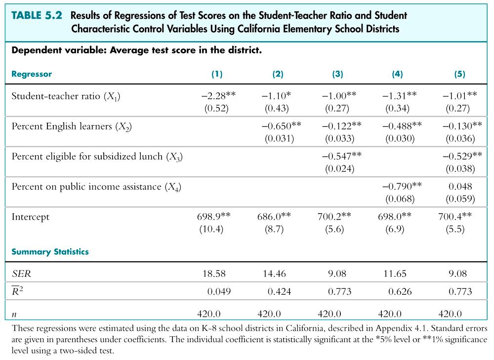
63 63

64 Summary: Multiple Regression Multiple regression allows you to estimate the effect on Y of a change in X1, holding X constant. If you can measure a variable, you can avoid omitted variable bias from that variable by including it. There is no simple recipe for deciding which variables belong in a regression you must exercise judgment. One approach is to specify a base model relying on a- priori reasoning then to explore the sensitivity of the key estimate(s) in alternative specifications. 64