Motivation for multiple regression

Transcription

1 Motivation for multiple regression 1. Simple regression puts all factors other than X in u, and treats them as unobserved. Effectively the simple regression does not account for other factors. 2. The slope coefficient β 1 in simple regression has causal interpretation only if the independent variable X is exogenous, i.e., cov(x, u) = 0. This is an assumption that we need to check. 3. The assumption cov(x, u) = 0 can be too strong to hold in reality. If any variable in u is correlated with X, the independent variable becomes endogenous, and the slope coefficient no longer has causal interpretation (in this case β 1 just measures association). 4. We can show that ˆβ 1 = (xi x)(y i ȳ) = (xi x) 2 (xi x)y i (1) (xi x) 2 = (xi x)(β 0 + β 1 x i + u i ) (xi x) 2 = β 1 + (xi x)u i (xi x) 2 (2) β The last result is important, and it implies that cov(x, u), (as n ) (3) σx 2 ˆβ 1 { β1, if cov(x, u) = 0 β 1 + bias, if cov(x, u) 0, bias = cov(x,u) σ 2 x (4) In words, the estimated slope coefficient converges to the true value (so is unbiased) if X is exogenous. When X becomes endogenous, ˆβ 1 is a biased estimate. The bias is given by cov(x,u). σx 2 6. One extreme case is β 1 = 0, so X has no causal effect on Y at all. But because X is correlated with some variables in the error term, the regression can produce a statistically significant ˆβ 1. In other words, the regression indicates spurious causality that does not exist. 7. For example, we may regress salary on education, and put ability in the error term. Because ability and education are correlated, the result of the simple regression may 1

2 be biased. What is captured by the simple regression may be the effect of ability on salary, not the effect of education on salary. 8. A multiple regression can explicitly account for many, if not all, other factors, by taking them out of the error term. Consider the simplest multiple regression Y = β 0 + β 1 X 1 + β 2 X 2 + e, (5) where e is the error term, for which we assume E(e X 1, X 2 ) = 0. (6) 9. This multiple regression becomes the simple regression if we define the error term in the simple regression as u β 2 X 2 + e. If we run the simple regression of Y on X 1 we can show ˆβ 1 β 1 + bias, bias = cov(x 1, u) σ 2 x1 = β 2 cov(x 1, X 2 ) σ 2 x1 (7) If β 2 > 0, cov(x 1, X 2 ) > 0, then bias > 0, ˆβ 1 > β 1, so the simple regression overestimates the effect of X 1 on Y. See Table 3.2 of the textbook for other possibilities. 10. We call X 2 the omitted variable if (i) it has causal effect on Y (so β 2 0), (ii) it is correlated with the key regressor (so cov(x 1, X 2 ) 0), and (iii) it is excluded from the regression (being put in the error term). The bias caused by omitted variable is called omitted variable bias. 11. If we use non-experimental data and the goal is to prove causality, omitted variable bias is the top issue we need to address. We have to ask if there is any variable in the error term which is the omitted variable. 12. Consider another example of omitted variable bias. Before we tried the simple regression of house price on the number of bathroom X 1. In that simple regression the error term contains the size of house X 2, which is the omitted variable. X 2 affects the house price, and is correlated with X 1. Therefore the slope of the simple regression is a biased estimate for the true causal effect of X 1 on Y. 2

3 Estimating multiple regression 1. Consider a multiple regression given by Y = β 0 + β 1 X 1 + β 2 X β k X k + u (1) Note there are k + 1 regressors, and one of them is constant (the intercept term). 2. The unknown parameters are β i, i = 0, 1,...k and σ 2 = var(u). 3. The key assumption to induce causality in multiple regression is E(u X 1, X 2,..., X k ) = E(u) = 0 (2) Assumption (2) is more likely to hold in reality than the simple regression because u now contains fewer variables. That means the multiple regression is more suitable than the simple regression for proving causality. 4. Notice that Assumption (2) does NOT require cov(x i X j ) 0. It is OK for the regressors in the multiple regression to be correlated with each other. Actually that is the whole point for multiple regression, which explicitly controls for X 2,..., X k and any one of them can be correlated with the key regressor X 1. Assumption (2) only requires those regressors be uncorrelated with the error term. 5. The OLS estimators for the coefficients, denoted by ˆβ k, (k = 0, 1,..., k), are obtained by solving k + 1 equations, which are the first order conditions (FOC) for minimizing residual sum squares i ûi = 0, (FOC 1) i x 1iû i = 0, (FOC 2)...,... i x kû i = 0, (FOC k+1) The formula for ˆβ k is complicated. Matrix algebra (not required) is needed in order to get simpler formula. 6. However, there is a simple formula for ˆβ 1 if we follow a two-step procedure (3) Theorem 1 Let ˆr be the residual of auxiliary regression of X 1 on X 2,..., X k. Then 1

4 the OLS estimator for β 1 in multiple regression (1) is ˆβ 1 = i ˆr iy i (Frisch-Waugh Theorem) (4) 7. Frisch-Waugh Theorem theorem indicates that we can obtain ˆβ 1 in two steps (a) Step 1: regress X 1 on X 2,..., X k and keep the residual ˆr (b) Step 2: regress Y on ˆr without intercept term 8. Residual ˆr measures the part of X 1 that cannot be explained by X 2,..., X k. Put differently, ˆr captures the part of X 1 after the effect of other factors has been netted out. This is why multiple regression is better than simple regression for proving causality. 9. Proof of Frisch-Waugh Theorem: Because ˆr is the residual, so it satisfies the FOC. That is and ˆr i = 0, i i ˆr i x 1i = i i x 2iˆr i = 0,..., i where û i is the residual for (1). The above equations imply that i ˆr iy i = ˆr 2 i, i ˆr i( ˆβ 0 + ˆβ 1 x 1i ˆβ k x ki + û i ) x kiˆr i = 0 (5) ˆr i û i = 0 (6) i = ˆβ 1 (7) 10. The OLS estimate and true coefficient are related via ˆβ 1 = β 1 + i ˆr iu i (8) from which we can prove the statistical property of ˆβ 1 : (a) E( ˆβ 1 X) = β 1 so ˆβ 1 is unbiased (b) The (conditional) variance for ˆβ 1 (assuming homoskedasticity) is var( ˆβ 1 X) = σ2 = σ 2 SST X1 (1 R 2 X1 ) (9) 2

5 where SST X1 = i (x 1i x 1 ) 2 measures the total variation in X 1, and RX1 2 denotes the R squared for the auxiliary regression of X 1 on X 2,..., X k. Everything else equal, the variance is big (and OLS estimate is imprecise) if X 1 is highly correlated with other independent variable (RX1 2 is big). The phenomenon of high correlation among regressors is called multicollinearity. The consequence of multicollinearity is insignificant estimate Intuitively, when regressors are highly correlated, the regression can not tell them apart, so the estimate is imprecise. 11. Now we face a trade off. The chance of multicollinearity is zero when we run simple regression. But simple regression has high chance of suffering omitted variable bias. Multiple regression has higher chance of multicollinearity, but lower chance of omitted variable bias. Econometrics puts more weight on omitted variable bias than multicollinearity 12. After obtaining the coefficient estimates, we can compute the residual û i = Y i Ŷi = Y i ˆβ 0 ˆβ 1 X 1i... ˆβ k X ki (10) Then the variance of the error term is estimated as ˆσ 2 = û2 i n k 1 (11) The square root of ˆσ 2 is called the standard error of regression (SER). 13. Because multiple regression has multiple independent variables, we can test hypothesis that involves several coefficients. The test is called F test, and is computed as F = (RSS r RSS u )/q RSS u /(n k u 1) (12) where RSS r is the RSS for the restricted regression that imposes the null hypothesis. RSS u is the RSS for the unrestricted regression, q is the number of restrictions, and k u is the number of regressors in the unrestricted regression. 3

6 (a) The F test follows F distribution with degree of freedom of (q, n k u 1) under the null hypothesis. The t test is special case of F test. The null hypothesis is rejected if the p-value is less than (b) The intuition is, the null hypothesis is false (so can be rejected) if imposing the null hypothesis significantly changes RSS. (c) For example, consider an unrestricted multiple regression Y = β 0 + β 1 X 1 + β 2 X 2 + u The null hypothesis is H 0 : β 1 = β 2 By imposing the restriction in the null hypothesis, we get the restricted regression Y = β 0 + β 1 (X 1 + X 2 ) + u so the restricted regression uses X 1 + X 2 as regressor. For this example q = 1 F test can be used when the null hypothesis involes several coefficients 4

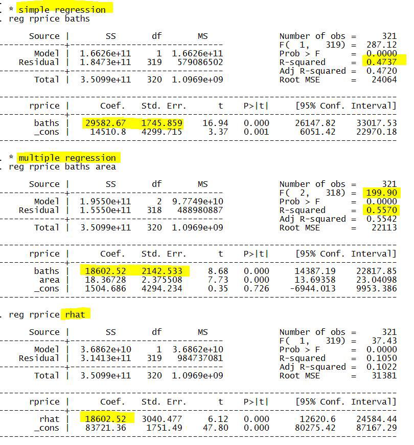
7 Example: Multiple Regression 1. We still use the house data. 2. First we run simple regression of rprice on baths. This simple regression puts variable area (which measures the size of house) into the error term. Because the number of bathrooms and house size must be correlated, baths is endogenous in the simple regression. As a result, the estimated coefficient of baths has NO causal interpretation (or is a biased estimate for the true causal effect). This number just measures the linear association or correlation between baths and rprice. We can only conclude that having one more bathroom is associated with a raise of in real house price. The OLS fitted line baths, however, is the best linear predictor for y (if we only use baths as predictor), no matter baths is exogenous or not. 3. Next we run multiple regression of rprice on baths and area. The stata command is reg rprice baths area. Now area is out of the error term, but other factors may still be there. That means it is still unlikely we can get causal effect by running this multiple regression with just two regressors. The estimated coefficient of baths now becomes , smaller than We can conclude that having one more bathroom, while holding house size fixed, is associated with a raise of in real house price. Put differently, if we have two houses with same size, but one house has one more bathroom than the other, then the rprice of former is higher than the latter by Another way to interpret is, it measures the association between baths and rprice, after the effect of area has been netted out. 4. So one benefit of multiple regression is that multiple regression can explicitly control for other factors, therefore lower the chance of omitted variable bias. Comparing the simple and multiple regressions, it is safe to say the simple regression (in this example) overestimates the effect of baths on rprice. The simple regression estimated coefficient may capture not just the effect of baths, but also area. In short, there is omitted variable bias for simple regression. The omitted variable is area. The omitted variable bias is positive since baths and area are positively correlated and we expect area has positive effect on rprice, see Table 3.2 in the textbook for detail. 5. Another benefit of multiple regression is bigger R squared. We see > The multiple regression fits data better just because it uses more regressors (more 1

8 information) 6. Multiple regression has cost. Note that in multiple regression the standard error for baths coefficient is , higher than in simple regression. This finding implies that the estimate in multiple regression is less precise than simple regression. It is the correlation between baths and area that causes the variance to rise, see formula below var( ˆβ 1 X) = σ2 = σ 2 SST X1 (1 R 2 X1 ). For this problem we are lucky because baths is still significant after area is included. In practice, it is not uncommon that the key regressor becomes insignificant after other regressors are added. 7. Next we apply the Frisch-Waugh Theorem to show how to obtain The stata commands are * step 1: auxiliary regression qui reg baths area predict rhat, re * step 2: regress y onto rhat reg rprice rhat So first we (quietly) regress baths X 1 onto area X 2, and save the residual rhat ˆr using command predict with option re. In step 2 we regress rprice Y onto rhat. We get the same estimate as that reported by command reg rprice baths area, so Frisch- Waugh Theorem is verified. 8. We also report the F test for the hypothesis that baths and size have same effect on rprice. The null hypothesis is H 0 : β 1 = β 2. You can use the command test baths = area. Or you can construct the F test manually by running unrestricted and restricted regressions. See the do file for details. 2

9 3

10 Do File * Do file for multiple regression (chapter 3 and 4) clear capture log close ************************************* cd "I:\311" log using 311log.txt, text replace use 311_house.dta, clear * simple regression reg rprice baths * multiple regression reg rprice baths area * save rss sca rssu = e(rss) * example of f test, H0: beta1 = beta2 test baths = area * restricted regression gen x = baths + area qui reg rprice x sca rssr = e(rss) * F test and p value sca f = ((rssr-rssu)/1)/(rssu/321-3) sca pvalue = Ftail(1, 318, f) dis "f test is " f dis "pvalue is " pvalue * verify Frisch-Waugh Theorem * step 1: auxiliary regression qui reg baths area predict rhat, re * step 2: regress y onto rhat reg rprice rhat ***************************************** log close 4