Chapter 3: Image Enhancement in the. Office room : 841

Transcription

1 Chapter 3: Image Enhancement in the Spatial Domain Lecturer: Jianbing Shen shenjianbing@bit.edu.cn Oice room : cn/shenjianbing

2 Principle Objective o Enhancement Process an image so that the result will be more suitable than the original image or a speciic c application. The suitableness is up to each application. A method which h is quite useul or enhancing an image ma not necessaril be the best approach or enhancing another images 2

3 2 domains Spatial Domain : image plane Techniques are based on direct manipulation o piels in an image Frequenc Domain : Techniques are based on modiing the Fourier transorm o an image There are some enhancement techniques based on various combinations o methods rom these two categories. 3

4 Good images For human visual The visual evaluation o image qualit is a highl hl subjective process. It is hard to standardize the deinition o a good image. For machine perception The evaluation task is easier. A good image is one which gives the best machine recognition results. A certain amount o trial and error usuall is required beore a particular image enhancement approach is selected. 4

5 Spatial Domain Procedures that operate directl on piels. g, = T[,] where, is the input image g, is the processed image T is an operator on deined over some neighborhood o, 5

6 Mask/Filter Neighborhood o a point, can be deined d b using a square/rectangular common, used or circular subimage area centered at, The center o the subimage is moved rom piel to piel starting at the top o the corner 6

7 Point Processing Neighborhood = 11 piel g depends on onl the value o at, T = gra level or intensit t or mapping transormation unction s = Tr Where r = gra level o, s = gra level o g, 7

8 Contrast Stretching Produce higher contrast than the original b darkening the levels below m in the original image Brightening the levels above m in the original image 8

9 Thresholding Produce a two-level binar image 9

10 Mask Processing or Filter Neighborhood is bigger than 11 piel Use a unction o the values o in a predeined neighborhood o, to determine the value o g at, The value o the mask coeicients determine the nature o the process Used in techniques Image Sharpening Image Smoothing 10

11 3 basic gra-level transormation unctions Negative nth root Log nth power Identit Inverse Log Input gra level, r Linear unction Negative and identit transormations Logarithm unction Log and inverse-log transormation Power-law unction n th power and n th root transormations 11

12 Identit unction Negative Log nth root nth power Output intensities are identical i to input intensities. Is included in the graph onl or completeness. Identit Inverse Log Input gra level, r 12

13 Image Negatives Negative nth root Log nth power Identit Inverse Log Input gra level, r An image with gra level in the range [0, L-1] where L = 2 n ; n = 1, 2 Negative transormation : s = L 1 r Reversing the intensit levels l o an image. Suitable or enhancing white or gra detail embedded in dark regions o an image, especiall when the black area dominant in size. 13

14 Log Transormations Negative nth root Log nth power Identit Inverse Log Input gra level, r s = c log 1+r c is a constant and r 0 Log curve maps a narrow range o low gra-level values in the input image into a wider range o output levels. Used to epand the values o dark piels in an image while compressing the higher-level values. 14

15 Log Transormations It compresses the dnamic range o images with ih large variations i in piel values Eample o image with dnamic range: Fourier spectrum image It can have intensit t range rom 0 to 10 6 or higher. We can t see the signiicant degree o detail as it will be lost in the displa. 15

16 Eample o Logarithm Image Fourier Spectrum with range = 0 to Result ater appl the log transormation with c = 1, range = 0 to

17 Inverse Logarithm Transormations Do opposite to the Log Transormations Used to epand the values o high piels in an image while compressing the darker-level values. 17

18 Power-Law Transormations Input gra level, r Plots o s = cr or various values o c = 1 in all cases s = cr c and are positive constants Power-law curves with ractional values o map a narrow range o dark input values into a wider range o output values, with the opposite being true or higher values o input levels. c = = 1 Identit unction 18

19 Gamma correction Monitor Gamma = 2.5 correction Monitor =1/2.5 = 0.4 Cathode ra tube CRT devices have an intensit-to-voltage response that is a power unction, with varing rom 1.8 to 2.5 The picture will become darker. Gamma correction is done b preprocessing the image beore inputting it to the monitor with s = cr 1/ 19

20 Another eample : MRI c d a b a a magnetic resonance image o an upper thoracic human spine with a racture dislocation and spinal cord impingement The picture is predominatel dark An epansion o gra levels are desirable needs < 1 b result ater power-law transormation with = 0.6, c=1 c transormation with = 0.4 best result d transormation with = 0.3 under acceptable level 20

21 Eect o decreasing ggamma When the is reduced too much, the image begins to reduce contrast to the point where the image started to have ver slight wash-out look, especiall in the background 21

22 Another eample a c b d a image has a washed-out appearance, it needs a compression o gra levels needs > 1 b result ater power-law transormation with = 3.0 suitable c transormation with = 4.0 suitable d transormation with = 5.0 high contrast, the image has areas that are too dark, some detail is lost 22

23 Piecewise-Linear Transormation Functions Advantage: The orm o piecewise unctions can be arbitraril comple Disadvantage: Their speciication requires considerabl more user input 23

24 Contrast Stretching increase the dnamic range o the gra levels in the image b a low-contrast image : result rom poor illumination, lack o dnamic range in the imaging sensor, or even wrong setting o a lens aperture o image acquisition c result o contrast stretching: r 1,s 1 = r min,0 and r 2,s 2 = r ma,l-1 d result o thresholding 24

25 Gra-level slicing Highlighting a speciic range o gra levels in an image Displa a high value o all gra levels l in the range o interest and a low value or all other gra levels a transormation highlights hl h range [A,B] o gra level and reduces all others to a constant t levell b transormation highlights range [A,B] but preserves all other levels l 25

26 Bit-plane slicing One 8-bit bte Bit-plane 7 most signiicant Bit-plane 0 least signiicant ii Highlighting the contribution made to total image appearance b speciic bits Suppose each piel is represented b 8 bits Higher-order bits contain the majorit o the visuall signiicant data Useul or analzing the relative importance plaed b each bit o the image 26

27 Eample The binar image or bit-plane 7 can be obtained b processing the input image with a thresholding gra-level transormation. Map all levels between 0 and 127 to 0 Map all levels between 129 and 255 to 255 An 8-bit ractal image 27

28 8 bit planes Bit-plane 7 Bit-plane 6 Bitplane Bit- Bit- 5 plane 4 plane 3 Bit- Bit- Bit- plane 2 plane 1 plane 0 28

29 Histogram Processing Histogram o a digital image with gra levels in the range [0,L-1] is a discrete unction Where r k : the k th gra levell hr k = n k n k : the number o piels in the image having gra level l r k hr k : histogram o a digital image with gra levels r k 29

30 Normalized Histogram dividing each o histogram at gra level r k b the total number o piels in the image, n For k = 0,1,,L-1 pr k = n k /n pr k gives an estimate o the probabilit o occurrence o gra level r k The sum o all components o a normalized histogram is equal to 1 30

31 Histogram Processing Basic or numerous spatial domain processing techniques Used eectivel or image enhancement Inormation inherent in histograms also is useul in image compression and segmentation 31

32 Eample Dark image Components o histogram are concentrated on the low side o the gra scale. Bright image Components o histogram are concentrated on the high h side o the gra scale. 32

33 Eample Low-contrast image histogram is narrow and centered toward themiddleothe gra scale High-contrast image histogram covers broad range o the gra scale and dthe distribution tib ti o piels is not too ar rom uniorm, with ver ew vertical lines being much higher than the others 33

34 Histogram Equalization As the low-contrast image s histogram is narrow and centered toward the middle o the gra scale, i we distribute the histogram to a wider range the qualit o the image will be improved. We can do it b adjusting the probabilit densit unction o the original histogram o the image so that the probabilit spread equall 34

35 Histogram transormation s k = Tr k s Tr 0 r k 1 r s = Tr Where 0 r 1 Tr satisies a. Tr is singlevalued and monotonicall increasingl in the interval 0 r 1 b. 0 Tr 1 or 0 r 1 35

36 Probabilit Densit Function The gra levels in an image ma be viewed as random variables in the interval [0,1] Probabilit Densit Function PDF is one o the undamental nt descriptors s o a random variable 36

37 Let Applied to Image p r r denote the PDF o random variable r p s s denote the PDF o random variable s I p r r and Tr are known and T - 1 s satisies condition a then p s s can be obtained using a ormula : p s s p r r dr ds 37

38 Applied to Image The PDF o the transormed variable s is determined b the gra-level PDF o the input image and b the chosen transormation unction 38

39 Transormation unction A transormation unction is a cumulative distribution unction CDF o random variable r : s r T r p w dw r 0 where w is a dumm variable o integration Note: Tr depends on p r r 39

40 Cumulative Distribution unction CDF is an integral o a probabilit unction alwas positive is the area under the unction Thus, CDF is alwas single valued and monotonicall increasing Thus, CDF satisies the condition a We can use CDF as a transormation unction 40

41 Finding p s s rom given Tr ds dr dt r dr r d p dr 0 p r p r r w dw p Substitute and ield s s p r dr r ds p r r p 1 r 1 where 0 s 1 r 41

42 p s s s As p s s is a probabilit unction, it must be zero outside the interval [0,1] in this case because its integral over all values o s must equal 1. Called p s s as a uniorm probabilit densit unction p s s is alwas a uniorm, independent o the orm o p r r 42

43 s r 0 T r p w dw r ields P s s a random variable s characterized b a uniorm probabilit unction s

44 Discrete transormation unction The probabilit o occurrence o gra level in an image is approimated b p r r k n n k where k 0, 1,..., L-1 The discrete version o transormation ti n k k n j sk T rk, pr r j where k 0, 1,..., L -1 n j0 j0 n 44

45 Histogram Equalization Thus, an output image is obtained b mapping each piel with level l r k in the input image into a corresponding piel with level s k in the output image In discrete space, it cannot be proved in general that this discrete transormation will produce the discrete equivalent o a uniorm probabilit densit unction, which would be a uniorm histogram 45

46 Eample beore ater Histogram equalization 46

47 Eample beore ater Histogram equalization The qualit is not improved much because the original image alread has a broaden gra-level scale 47

48 Eample No. o piels image Gra scale = [0,9] histogram Gra level 48

49 Gra Levelj No.o piels nj s k j n j k j0 n s 9 j n New gra 0 0 level j / / / / / / / /

50 Eample No. o piels Output image Gra scale = [0,9] Gra level Histogram equalization 50

51 Note It is clearl seen that Histogram equalization distributes ib t the gra level l to reach the maimum gra level white because the cumulative distribution unction equals 1 when 0 r L-1 I the cumulative numbers o gra levels are slightl dierent, the will be mapped to little dierent or same gra levels as we ma have to approimate the processed gra level o the output image to integer number Thus the discrete transormation unction can t guarantee the one to one mapping relationship 51

52 Result image and its histogram The output image s histogram Original image Ater applied the histogram equalization Notice that the output histogram s low end has shited right toward the lighter region o the gra scale as desired. 52

53 Note Histogram speciication is a trial-anderror process There are no rules or speciing histograms, and one must resort to analsis on a case-b-case s basis or an given enhancement task. 53

54 Note Histogram processing methods are global processing, in the sense that piels are modiied b a transormation on unction based on the gra-level content o an entire image. Sometimes, we ma need to enhance details over small areas in an image, which is called a local enhancement. 54

55 Local Enhancement a b c a Original image slightl blurred to reduce noise b global histogram equalization enhance noise & slightl increase contrast but the construction is not changed c local histogram equalization using 77 neighborhood reveals the small squares inside larger ones o the original image. deine a square or rectangular neighborhood and move the center o this area rom piel to piel. at each location, the histogram o the points in the neighborhood h is computed and either histogram equalization or histogram speciication transormation unction is obtained. another approach used to reduce computation is to utilize nonoverlapping regions, but it usuall produces an undesirable checkerboard eect. 55

56 Eplain the result in c Basicall, the original image consists o man small squares inside the larger dark ones. However, the small squares were too close in gra level to the larger ones, and their sizes were too small to inluence global histogram equalization signiicantl. So, when we use the local l enhancement technique, it reveals the small areas. Note also the iner noise teture is resulted b the local processing using relativel small neighborhoods. 56

57 Enhancement using Arithmetic/Logic Operations Arithmetic/Logic operations perorm on piel b piel basis between two or more images ecept NOT operation which perorm onl on a single image 57

58 Logic Operations Logic operation perorms on gra-level images, the piel values are processed as binar numbers light represents a binar 1, and dark represents a binar 0 NOT operation = negative transormation 58

59 Eample o AND Operation original image AND image mask Figure 3.27 result o AND operation 59

60 Eample o OR Operation original image Figure 3.27 OR image mask result o OR operation 60

61 Image Subtraction g, =, h, enhancement o the dierences between images 61

62 Image Subtraction a c b d a. original ractal image b. result o setting the our lower-order bit planes to zero reer to the bit-plane slicing the higher planes contribute signiicant detail the lower planes contribute more to ine detail image b. is nearl identical visuall to image a, with a ver slightl drop in overall contrast due to less variabilit o the gra-level values in the image. c. dierence between a. and b. nearl black d. histogram equalization o c. perorm contrast stretching transormation 62

63 Mask mode radiograph mask image an image taken ater injection o a contrast medium iodine into the bloodstream with mask subtracted out. Note: the background is dark because it doesn t change much in both images. the dierence area is bright because it has a big change h, is the mask, an X-ra image o a region o a patient s bod captured b an intensiied TV camera instead o traditional X- ra ilm located opposite an X-ra source, is an X-ra image taken ater injection a contrast medium into the patient s bloodstream images are captured at TV rates, so the doctor can see how the medium propagates through the various arteries in the area being observed the eect o subtraction in a movie showing mode.

64 Note We ma have to adjust the gra-scale o the subtracted image to be [0, 255] i 8-bit is used irst, ind the minimum gra value o the subtracted image second, ind the maimum gra value o the subtracted image set the minimum value to be zero and the maimum to be 255 while the rest are adjusted according to the interval [0, 255], b timing each value with 255/ma Subtraction is also used in segmentation o moving pictures to track the changes ater subtract the sequenced images, what is let should be the moving elements in the image, plus noise 64

65 Image Averaging g consider a nois image g, ormed b the addition o noise, to an original image, g, =, +, 65

66 Image Averaging g i noise has zero mean and be uncorrelated then it can be shown that i g, = image ormed b averaging K dierent nois images 1 K g, 1 K K i 1 g i, 66

67 Image Averaging g then 1 2 g, K K 2, 2 g,, 2, = variances o g and i K increase, it indicates that the variabilit noise o the piel at each location, decreases. 67

68 thus Image Averaging g E { g, }, E { g, } = epected value o g output ater averaging g = original image, 68

69 Image Averaging g Note: the images g i, nois images must be registered aligned in order to avoid the introduction on o blurring and other artiacts in the output image. 69

70 Eample a c e b d a original image b image corrupted b additive Gaussian noise with zero mean and a standard deviation o 64 gra levels. c. -. results o averaging K = 8, 16, 64 and 128 nois images 70

71 Spatial Filtering use ilter can also be called as mask/kernel/template or window the values in a ilter subimage are reerred to as coeicients, rather than piel. our ocus will be on masks o odd sizes, e.g. 33, 55, 71

72 Spatial Filtering Process simpl move the ilter mask rom point to point in an image. at each point,, the response o the ilter at that point is calculated using a predeined d relationship. R w z w z... R mn w i z i ii w mn z mn 72

73 Linear Filtering Linear Filtering o an image o size MN ilter mask o size mn is given b the epression the epression a b t s t s w g a t b t t s t s w g,,, where a = m-1/2 and b = n-1/2 To generate a complete iltered image this equation must 73 To generate a complete iltered image this equation must be applied or = 0, 1, 2,, M-1 and = 0, 1, 2,, N-1

74 FIGURE 3.32 The mechanics o spatial iltering. The magniied drawing shows a 3*3 mask and the image section directl under it; the image section is shown displaced out rom under the mask or ease o readabilit.

75 Moving Average in 2D , g,

76 Moving Average in 2D , g,

77 Moving Average in 2D , g,

78 Moving Average in 2D , g,

79 Moving Average in 2D , g,

80 Moving Average in 2D , g,

81 Smoothing Spatial Filters used or blurring and or noise reduction blurring is used in preprocessing steps, such as removal o small details rom an image prior to object etraction bridging o small gaps in lines or curves noise reduction can be accomplished b blurring with a linear ilter and also b a nonlinear ilter 81

82 Smoothing Linear Filters output is simpl the average o the piels contained in the neighborhood o the ilter mask. called averaging g ilters or lowpass ilters. 82

83 Smoothing Linear Filters replacing the value o ever piel in an image b the average o the gra levels in the neighborhood will reduce the sharp transitions in gra levels. sharp transitions random noise in the image edges o objects in the image thus, smoothing can reduce noises desirable and blur edges undesirable 83

84 33 Smoothing Linear Filters bo ilter weighted average the center is the most important and other piels are inversel weighted as a unction o their distance rom the center o the mask 84

85 Weighted average ilter the basic strateg behind weighting the center point the highest and then reducing the value o the coeicients c ents as a unction o increasing distance rom the origin is simpl an attempt to reduce blurring in the smoothing process. 85

86 General orm : smoothing mask g ilter o size mn m and n odd a b t s t s w b a s b t t s t s w g,,, a b t s w g,, a s b t summation o all coeicient o the mask 86 summation o all coeicient o the mask

87 Eample a c e b d a. original image piel b. -. results o smoothing with square averaging ilter masks o size n = 3, 5, 9, 15 and 35, respectivel. Note: big mask is used to eliminate small objects rom an image. the size o the mask establishes the relative size o the objects that will be blended with the background. 87

88 Eample original image result ater smoothing with 1515 averaging mask result o thresholding we can see that the result ater smoothing and thresholding, the remains are the largest and brightest objects in the image. 88

89 Order-Statistics Filters Nonlinear Filters the response is based on ordering ranking the piels contained in the image area encompassed b the ilter eample median ilter : R = median{z k k = 1,2,,n n} ma ilter : R = ma{z k k = 1,2,,n n} min ilter : R = min{z k k = 1,2,,n n} note: n nis the size o the mask 89

90 Median Filters replaces the value o a piel b the median o the gra levels l in the neighborhood h o that piel the original value o the piel is included in the computation o the median quite popular p because or certain tpes o random noise impulse noise salt and pepper noise, the provide ecellent noise-reduction capabilities, with considering less blurring than linear smoothing ilters o similar size. 90

91 Median Filters orces the points with distinct gra levels to be more like their neighbors. isolated clusters o piels that are light or dark with respect to their neighbors, and whose area is less than n 2 /2 one-hal the ilter area, are eliminated b an n n median ilter. eliminated = orced to have the value equal the median intensit o the neighbors. larger clusters are aected considerabl less 91

92 Eample : Median Filters 92

93 Sharpening Spatial Filters to highlight ine detail in an image or to enhance detail that has been blurred, either in error or as a natural eect o a particular method o image acquisition. 93

94 Blurring vs. Sharpening as we know that blurring can be done in spatial domain b piel averaging in a neighbors since averaging is analogous to integration thus, we can guess that the sharpening must be accomplished b spatial dierentiation. 94

95 Derivative operator the strength o the response o a derivative operator is proportional to the degree o discontinuit o the image at the point at which h the operator is applied. thus, image dierentiation enhances edges and other discontinuities noise deemphasizes area with slowl varing gra-level values. 95

96 First-order derivative a basic deinition o the irst-order derivative o a one-dimensional unction is the dierence 1 96

97 Second-order derivative similarl, we deine the second-order derivative o a one-dimensional unction is the dierence

98 Derivative computation In discrete domain, the gradients o an image I along and directions at an piel poisiton j,i are deined as: 1 Forward dierences 前向差分法 Gj,i = Ij,i+1 - Ij,i Gj,i = Ij+1,i- Ij,i 2 Backward dierences 后向差分法 Gj,i = Ij,i - Ij,i-1 Gj,i = Ij,i - Ij-1,i 3 Central dierences 中心差分法 Gj,i = Ij,i+1 - Ij,i-1 Gj,i = Ij+1,i - Ij-1,i 98

99 First and Second-order First and Second-order derivative o, when we consider an image unction o two variables,,, at which time we will dealing with partial derivatives along w ll deal ng w th part al der vat ves along the two spatial aes.,,, Gradient operator 2 2 2,, Laplacian operator ,, linear operator

100 Discrete Form o Laplacian p rom, 2 1, 1, 2 2, 2 1, 1, 2 ield, 2 ] , 1, [ ], 4 1, 1,

101 Result Laplacian mask 101

102 Laplacian mask implemented an etension o diagonal neighbors 102

103 Other implementation o Laplacian masks give the same result, but we have to keep in mind that when combining add / subtract a Laplacian-iltered image with another image. 103

104 Eect o Laplacian Operator as it is a derivative operator, it highlights gra-level discontinuities in an image it deemphasizes regions with slowl varing gra levels tends to produce images that have graish edge lines and other discontinuities, all superimposed on a dark, eatureless background. 104

105 Correct the eect o eatureless background easil b adding the original and Laplacian image. be careul with the Laplacian ilter used 2,, g, 2,, i the center coeicient o the Laplacian mask is negative i the center coeicient o the Laplacian mask is positive 105

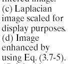
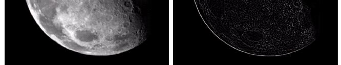
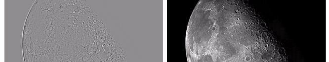
106 Eample a. image o the North pole o the moon b. Laplacian-iltered image with c. Laplacian image scaled or displa purposes d. image enhanced b addition with original i image

107 Mask o Laplacian + addition to simpl the computation, we can create a mask which do both operations, Laplacian an Filter and Addition the original image. 107

108 Mask o Laplacian + addition p 1, 1, [,, g ], 4 1, 1, 1, 1, [,, g 1] 1 1, 1, [, 5 1], 1,

109 Eample 109

110 ,, g, Note, 2, = =

111 Unsharp masking s,,, sharpened image = original image blurred image to subtract a blurred version o an image produces sharpening output image. 111

112 High-boost iltering g g A,,, A hb 1 A hb,, 1,,, 1, A A s hb generalized orm o Unsharp masking A A 1

113 High-boost iltering g g 1 A i we use Laplacian ilter to create,, 1, A s hb i we use Laplacian ilter to create sharpen image s, with addition o i i l i original image 2,,, 2 2 s 113,,

114 High-boost iltering ields i the center coeicient o the Laplacian mask is negative A,,, hb A, 2, 2 i the center coeicient o the Laplacian mask is positive 114

115 High-boost Masks A 1 i A = 1, it becomes standard d d Laplacian sharpening 115

116 Eample 116

117 Gradient Operator G G irst derivatives are implemented using the magnitude o the gradient. mag 2 [ G 2 2 G ] 1 2 the magnitude becomes nonlinear commonl appro. G G 117

118 z 1 z 2 z 3 Gradient Mask z 4 z 5 z 6 z 7 z 8 z 9 simplest approimation, and z z G z z G and z z G z z G ] [ ] [ z z z z G G z z z z 118

119 z 1 z 2 z 3 Gradient Mask z 4 z 5 z 6 z 7 z 8 z 9 Roberts cross-gradient operators, and z z G z z G ] [ ] [ z z z z G G ] [ ] [ z z z z G G z z z z z z z z 119

120 Gradient Mask Sobel operators, 33 G G z 1 z 2 z 3 z 4 z 5 z 6 z 7 z 8 z 9 z 2z z z 2z z z 2z z z 2z z G G the weight value 2 is to achieve smoothing b giving more important to the center point 120

121 Note the summation o coeicients in all masks equals 0, indicating that the would give a response o 0 in an area o constant gra level. 121

122 Eample 122

123 Eample o Combining Spatial Enhancement Methods want to sharpen the original i image and bring out more skeletal l detail. problems: narrow dnamic range o gra level and high noise content makes the image diicult to enhance 123

124 Eample o Combining Spatial Enhancement Methods solve : 1. Laplacian to highlight ine detail 2. gradient to enhance prominent edges 3. gra-level transormation to increase the dnamic range o gra levels 124

125 125

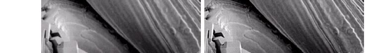
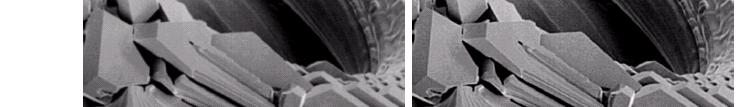
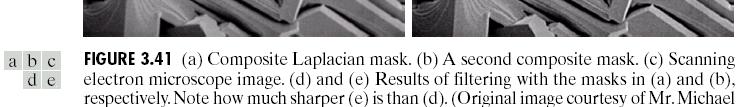
126 126