PROPAGATION DYNAMICS OF SPATIO-TEMPORAL WAVE PACKETS

Transcription

1 PROPAGATION DYNAMICS OF SPATIO-TEMPORAL WAVE PACKETS Thesis Submitted to The School of Engineering of the UNIVERSITY OF DAYTON In Partial Fulfillment of the Requirements for The Degree of Master of Science in Electro-Optics By Qian Cao UNIVERSITY OF DAYTON Dayton, Ohio August, 24

2 PROPAGATION DYNAMICS OF SPATIO-TEMPORAL WAVE PACKETS Name: Cao, Qian APPROVED BY: Andy Chong, Ph.D. Advisor Committee Chairman Assistant Professor, Department of Physics Joseph Haus, Ph.D. Committee Member Professor, Electro-Optics Graduate Engineering Program Partha Banerjee, Ph.D. Committee Member Professor, Electro-Optics Graduate Engineering Program John G. Weber, Ph.D. Associate Dean School of Engineering Eddy M. Rojas, Ph.D., M.A., P.E. Dean, School of Engineering ii

3 c Copyright by Qian Cao All rights reserved 24

4 ABSTRACT PROPAGATION DYNAMICS OF SPATIO-TEMPORAL WAVE PACKETS Name: Cao, Qian University of Dayton Advisor: Dr. Andy Chong We measured the three-dimensional (3D) propagation dynamics of the Airy-Bessel wave packet, inculding its intensity and phase evolution. Its non-diffraction and non-dispersive features were verified. Meanwhile, we built a spatial light modulator (SLM) based wave packet shaping system to generate other types of wave packets such as Airy-Airy-Airy and dual-airy-airy-rings. These wave packets were also measured in 3D. The abrupt 3D autofocusing effect was observed on dual-airy- Airy-rings. iii

5 To my family, my advisor and committee members and the time in University of Dayton. iv

6 ACKNOWLEDGMENTS First of all, I want to express my thank to my advisor, Prof. Andy Chong. Although the time when I became his student it was the second year of his professor career, he taught and guided me in the world of science in such an experienced way. Without his guidance cannot I become so interested in physics. His enthusiasm in science, his broad knowledge and the encouragement is invaluable in my research. At the same time, I want to thank my committee members, Prof. Joseph Haus and Prof. Partha Banerjee for their guidance and patience. It was my fortune and pleasure to work in Dr. Chong s ultrafast laser group. I sincerely thank Chenchen Wan, Xin Huang and Peiyun Li, the group members, who have contributed a lot in my research. Without their help and company, I will not have the courage to accomplish this work. Finally I sincerely thank my family. I am indebted forever for their priceless love and support. They have been asking about the progress of my thesis for long. I believe as I finish the thesis writing, the story will come to a happy ending. v

7 TABLE OF CONTENTS ABSTRACT iii DEDICATION iv ACKNOWLEDGMENTS v LIST OF FIGURES INTRODUCTION Organization of the thesis Introduction THEORETICAL BACKGROUND Optical Airy wave Airy pulse Airy beam and other types of Airy wave Bessel beam THREE-DIMENSIONAL MEASUREMENT SYSTEM Mechanism and mathematical background Experimental configuration Temporal phase retrieval MEASUREMENT RESULTS Propagation dynamics of Airy-Bessel wave packet Experiment parameters D intensity before propagation D intensity after propagation Temporal phase retrieval Measurement of Airy-Airy-Airy wave packet Measurement of dual-airy-airy-rings wave packet CONCLUSIONS BIBLIOGRAPHY vii vi

8 LIST OF FIGURES 2. Airy pulse simulation Airy pulse propagation simulation under the influence of normal dispersion Airy beam simulation dual Airy pulse simulation Bessel beam simulation Axicon to generate Bessel beam Conceptual sketch of the measurement system Experimental setup for Airy-Bessel wave packet Experimental setup for general spatio-emporal wave packet Conceptual sketch of temporal phase retrieval Experiment parameters for Airy-Bessel measurements Results of the Airy-Bessel wave packet before propagation Results of the Airy-Bessel wave packet after propagation Temporal phase results for Airy-Bessel wave packet Experimental parameters for Airy-Airy-Airy measurements Results of the Airy-Airy-Airy wave packet vii

9 4.7 Temporal phase retrieval of Airy-Airy-Airy wave packet Experimental parameters for dual-airy-airy-rings measurements Results of the dual-airy-airy-rings wave packet at the Fourier plane Results of the dual-airy-airy-rings wave packet at the autofocus plane viii

10 CHAPTER INTRODUCTION The main theme of this thesis is the study of the propagation dynamics of spatio-temporal wave packets. The Airy-Bessel wave packet is the main wave packet to be studied in the thesis. Other wave packets such as Airy-Airy-Airy and dual-airy-airy-rings are also investigated.. Organization of the thesis There are be five chapters in this thesis. Chapter is the introduction to the research on optical spatio-temporal wave packets. It explains why they are an important research subject. This chapter gives an initial description of the measurement techniques used in this thesis and how they differ from conventional pulse measurement techniques. Finally, it ends with a brief description of wave packets specific to those studied in this thesis. Chapter 2 is the theoretical background for the spatio-temporal wave packets. Airy pulses, Bessel beams and other types of optical Airy waves are discussed in this chapter. For an Airy pulse, its mathematical form and unique properties such as self-healing and self-acceleration is explained. All the contents are in the words of optics to make it straightforward to understand how to realizes Airy pulses optically. For Bessel beams, the origin of the non-diffracting property is explained. Other optical realizations of Airy waves are introduced in the last section of this chapter.

11 Chapter 3 is the discussion around the three-dimensional (3D) measurement system. Firstly, the mathematics and the experimental configuration of this 3D measurement technique is briefly introduced. There are two different setups presented. One of them is used to generate the Airy- Bessel wave packet and measure its intensity profile in 3D. The other one is used to generate wave packets such as Airy-Airy-Airy and dual-airy-airy-rings. These two wave packets are measured in 3D and presented in the measurement results chapter. Finally the process of temporal phase retrieval is explained. This temporal phase retrieval technique is accurately a byproduct of the 3D measurement. Although some assumption must be made to access the temporal phase retrieval, this method can reveal the temporal phase signature with a good agreement with theoretical predictions. The temporal phase results are also presented in the measurement results chapter. Chapter 4 presents the 3D measurement results, as well as the temporal phase retrieval of the Airy-Bessel wave packet and the Airy-Airy-Airy wave packet. As the main theme of this thesis, the propagation dynamics of Airy-Bessel wave packet is studied in details covering from the experimental parameters to the 3D intensity profile and the temporal phase profile. For an Airy-Airy-Airy wave packet, its 3D intensity profile and its temporal phase is shown. For a dual-airy-airy-rings wave packet, to the best of our knowledge, it is the first time that such wave packet is experimentally generated. The 3D autofocusing effect is observed and measured in 3D. Chapter 5 states the conclusions, as the last chapter of this thesis..2 Introduction Spatio-temporal wave packets have demonstrated their potential in the field of nonlinear science, plasma generation [, 2], laser machining [3] and other scientific researches [4]. Combining some specific pulse shape and beam profile, these wave packets can have unique properties such as self-acceleration [5], self-healing [6], lateral acceleration [7], non-diffracting [8 ] and abrupt 2

12 autofocusing []. With these properties, spatio-temporal wave packets can serve as a powerful tool in various applications. Itself has also become an interesting research topic. To utilize and study those wave packets, it is necessary to learn how to measure them. Conventional measurement techniques include auto-correlation [2], cross-correlation and charge-coupled devices (CCD) camera. They are easy to implement. However, spatio-temporal coupled wave packets cannot be resolved by these methods. To overcome this, methods based on frequency-resolved optical gating (FROG) [3] and some other techniques with nonlinear processes [4] are developed. But these methods have restrictions on the type of the wave packets, wave packets energy and their spectrum bandwidth. These restrictions make the measurement scenarios highly limited. Later on, an interferometric measurement system based on noncollinear first order cross correlation is suggested [5 7]. This system can measure 3D intensity profile of spatio-temporal wave packets at various wavelengths. Recently its capability to measure the temporal phase is demonstrated [8]. The 3D measurements in this thesis are all achieved by using this measurement technique. Conventional methods will be used as a supplement and for comparison purpose. The wave packets to be studied in this thesis are Airy-Bessel, Airy-Airy-Airy and dual-airy- Airy-rings. An Airy-Bessel wave packet has been studied as a linear light bullet since it can propagate without dispersion or diffraction in the linear regime [9]. An Airy-Airy-Airy wave packet also belongs to the family of linear light bullet s. It has been studied both in the linear and the nonlinear regime [2]. A dual-airy-airy-rings wave packet is a wave packet which has been just recently proposed [2]. It can autofocus in an abruptly way which can be useful in some applications such as bio-imaging. The next chapter discusses the theories for Airy waves and Bessel beams. 3

13 CHAPTER 2 THEORETICAL BACKGROUND In this chapter, the theoretical background for optical spatio-temporal wave packets is covered. Airy pulses, Bessel beams and other types of optical Airy waves are discussed. The threedimensional (3D) measurement system is introduced in the next chapter and the 3D measurement results are presented in the fourth chapter. 2. Optical Airy wave An Airy wave is initially studied in the context of quantum mechanics. It has been proved that a wave function (ψ) in the form of an Airy function can propagate in free space without distortion and with constant acceleration [22]. It has also been proved that the Airy packet can preserve its integrity under the influence of a force F (t). Since the Schrödinger equation used in quantum mechanics is entirely analogous to the paraxial approximation of the Helmholtz wave equation, Airy waves can also studied in the context of optics. It has been proposed that a two dimensional (2D) Airy beam can propagation free of diffraction and it can self-accelerate in free space. After the first realization of 2D Airy beam [23], an Airy beam has been studied in its unique properties such as self-acceleration [23] and self-healing [6], in the paraxial regime [5] and the non-paraxial regime as well [24]. Later on, Airy pulses have been suggested [7] and it is pointed out that an Airy pulse can keep its shape under the influence of dispersion. These days, optical realizations of Airy waves 4

14 has become a big research topic. In the following sections, the mathematics behind Airy pulses and other type of Airy waves are explained. 2.. Airy pulse Before explaining the mathematics of Airy pulses, it is necessary to introduce some physical parameters which have been used to characterize the optical pulse. Due to the intrinsic Fourier transform property, a broad optical spectrum is needed to have an ultrafast optical pulse. The optical spectrum is determined by two physical parameters, its amplitude and its phase. These two parameters are defined through Ẽ(ω) = A(ω) exp(i φ(ω)), (2.) where A(ω) is the amplitude term and φ(ω) is the phase term. It is of note that the carrier frequency of an optical field is usually at the PHz level ( PHz = 5 Hz). For example, the carrier frequency of light at µm wavelength has an angular carrier frequency of.88 PHz. For simplicity, we assume ω = ω ω in Eqn. 2., where ω is the real optical frequency and ω is the center frequency. The phase term φ(ω) can be Taylor expanded around the center frequency [25]. Mathematically it can be written as φ(ω) = β(ω) z = β + β ω z + 2 β 2ω 2 z + 6 β 3ω 3 z +, (2.2) where β m = ( d m ) β dω m (m =,, 2,...). (2.3) β(ω) in Eqn. 2.2 is the propagation constant of the optical field, which has been widely used in waveguide optics and ultrafast optics. In a dispersive medium β(ω) = 2π λ n(ω), where n(ω) is the refractive index of the medium and λ is the wavelength of the optical field. β m in Eqn. 2.3 is the m th order Taylor expansion coefficient of the propagation constant around the center frequency. 5

15 β is related to the group velocity, which describes how fast ultrafast pulse propagates in the medium. When a localized coordinate is used (which means the observer moves with the pulse), β does not play a significant role analyzing the evolution of the ultrafast pulse (unless two pulses with different center frequency travel together, but this is not the case in this thesis). β 2 is called the group velocity dispersion (GVD) coefficient. When there is no phase variation on φ(ω) (φ(ω) = constant), an ultrafast pulse with a finite spectrum is called a Fourier transformlimited (TL) pulse. As a TL pulse propagates through a dispersive medium, the temporal pulse width broadens due to the influence of GVD. The broadening occurs whether the pulse is in a normal dispersive medium, β 2 >, and in an anomalous dispersive medium, β 2 < ; the distinction between the two GVD cases is in the advancement or lagging of the pulse s frequency spectrum (higher frequency components blue lags lower frequency components red in normal GVD media and red lags blue in anomalous GVD media). β 3 is the third order dispersion (TOD) coefficient. When the spectrum of an optical pulse is broad enough, TOD effect cannot be ignored. Higher order dispersion effects such as the fourth order dispersion play little roles so that they are not taken into consideration in this thesis. For a rigorous Airy wave, its spectrum consists an uniform amplitude and a cubic phase, which can be written as Ẽ(ω) = exp( i 6 β 3ω 3 z ), (2.4) where β 3 and z are constants. However the wave form as in Eqn. 2.4 is not square integrable, i.e. it does not have any physical meaning. An aperture is needed to bound the total energy. In the form of an Airy pulse, the aperture is the optical spectrum. Thus a truncated Airy pulse has a finite spectrum which can be written as Ẽ(ω) = A(ω) exp( i 6 β 3ω 3 z ). (2.5) 6

16 A(ω) (a.u.) ω (PHz).9 (a) Angular frequency spectrum Intensity (a.u.) Time (ps).5 (b) Fourier transform-limited pulse Intensity (a.u.) Time (ps).5 (c) Airy pulse Figure 2.: Airy pulse simulation. More detailed derivation can be found in this reference [7]. Fig. 2. gives simulation results to help to understand Airy pulses. Fig. 2.(a) is the spectrum of the optical field. It is centered at.83 PHz (corresponding to.3 µm) and has a Gaussian distribution. Fig. 2.(b) is the TL form pulse of this spectrum. By adding TOD phase, Airy pulse can be formed as shown in Fig. 2.(c). It is of note that there is a π phase shift between each lobe of the Airy pulse. This is a signature of Airy pulse. More generally speaking, this is the signature of Airy waves. When an Airy pulse propagates through a dispersive medium with GVD coefficient β 2 for a distance z, an extra GVD is added. The phase of the spectrum φ(ω) becomes Ẽ(ω) = A(ω) exp(i ( 6 β 3ω 3 z + 2 β 2ω 2 z + β ωz)) = A(ω) exp(i ( 6 β 3z (ω + β 2z ) 3 + (β β2 2z )(ω + β 2z ) z + C)), β 3 z 2 β 3 z β 3 z (2.6) where C is some constant phase. This constant is not of our interest in this thesis. Some conclusions can be made from Eqn Firstly, the linear phase term (β β2 2z )(ω + 2 β 3 z β 2 z ) z will result in a shift in the time domain. This property is called self-acceleration. The β 3 z direction of self-acceleration depends on the sign of β 3 z, which is the initial TOD. 7

17 Intensity (a.u.).5 Intensity (a.u.).5 2 Time (ps) 4 L D 5 2 Time (ps) 2 L D 5 (a) Pulse evolution with initial positive TOD (b) Pulse evolution with initial negative TOD Figure 2.2: Airy pulse propagation simulation under the influence of normal dispersion. Secondly, the center frequency will shift by an amount of ω = β 2z β 3 z. When the new center frequency is within the bandwidth of the optical spectrum, the Airy pulse can partially keep its shape. In other word, the influence of dispersion is reduced. Since ω is inversely proportional to the initial TOD, adding more initial TOD can enhance such dispersion-free property. Equivalently, having a broader spectrum will benefit it as well (an infinite broad spectrum can have this dispersionfree property forever). Some other simulation results about the pulse evolution under GVD are shown in Fig The z-axis of this graph is the normalized intensity. The x-axis is a localized time scale. And the y-axis is plotting with respect to the dispersion length. The dispersion length, similar with the diffraction length (Rayleigh range), is a parameter to characterize the dispersion effect. It is defined as L D = t2 β 2, (2.7) 8

18 (a) Initial Gaussian beam (b) Phase mask in the k-space (c) 2D Airy beam Figure 2.3: Airy beam simulation. where t is the width of the field via E(t) = exp( t2 t 2 ) and β 2 is the GVD coefficient of the dispersive medium where pulse propagates. Here t is determined by the main lobe of the Airy pulse. From the graphs, the self-acceleration effect is evident. With different sign of initial TOD, an Airy pulse will self-accelerate towards different directions. The Airy pulse can maintain its shape within 3 times the dispersion length. After propagation for 3 dispersion lengths, the Airy pulse starts to lose its shape. Finally the pulse evolution gets dominated by GVD effect Airy beam and other types of Airy wave Similarly a phase mask can be designed and applied to convert the transverse spatial profile of an optical field to approximate a 2D Airy beam [5, 26]. Fig. 2.3 illustrates the progression how a Gaussian beam will evolve when a cubic phase mask is added to its reciprocal space (k-space). Fig. 2.3(a) shows the intensity profile of a Gaussian beam with a beam diameter of mm. Fig. 2.3(b) is the cubic phase mask added in the k-space of such Gaussian beam. The mathematical expression 9

19 Intensity (a.u.) Time (ps) Intensity (a.u.) Time (ps) Intensity (a.u.) Time (ps) Intensity (a.u.) 2 5 Time (ps) GVD ( 5 3 fs 2 ) (a) Initial Gaussian (b) Dual Gaussian (c) Dual Airy (d) evolution of dual Airy under normal GVD Figure 2.4: dual Airy pulse simulation. of this phase mask can be written as ϕ(k x, k y ) (k 3 x + k 3 y), (2.8) where k x and k y are the coordinate in the reciprocal space. Reciprocal means in the Fourier domain. The Fourier transform of a Gaussian beam still has a Gaussian distribution. Fig. 2.3(c) shows the 2D Airy beam when such phase mask is applied. The optical Fourier transform can be accomplished by a single lens system. This property can be found in Fourier optics textbooks [27, 28]. Recalling Fig. 2.2, Airy pulses with different signs of initial TOD will self-accelerate towards different directions under normal dispersion (β 2 > ). This phenomenon is evident in Eqn. 2.6 since the sign of the change of the linear term β = β2 2z is dependent on the sign of β 3. One may 2 β 3 z ask: what would happen when two Airy pulses co-propagate in a dispersive medium? To answer this question it is necessary for us to know how to generate such dual Airy pulse. An illustration showing the progression from Gaussian to dual Gaussian to dual Airy pulses are shown in Fig A Gaussian pulse is presented in Fig. 2.4(a). A linear phase in the frequency domain of such pulse delays the pulse in the time domain by a certain shift. Similarly, a triangle shape phase in the frequency shifts two pulses in different directions, as shown in Fig.2.4(b). By adding cubic phase with different signs in each half of this spectrum, dual Airy pulses can be

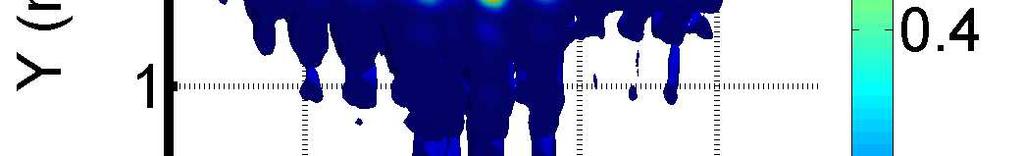
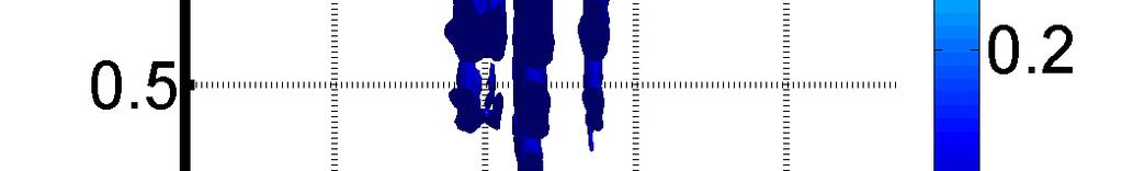
20 generated, as presented in Fig. 2.4(c). Now it is possible to numerically study the evolution of such dual Airy pulses under the influence of normal GVD. The result is shown in Fig. 2.4(d). Two Airy pulses will counter self-accelerate towards the center. At some point, a higher peak intensity can be formed. The peak intensity can be as high as 2 times the initial peak intensity. This feature might be useful in some applications. A radially symmetric phase third-order phase profile in the optical beam s Fourier domain can also be examined. The phase mask can be mathematically written as ϕ(r) = a r + b (r ) 3, (2.9) where r is the radius in a polar coordinate, is a constant displancement, a and b are phase coefficients. When this phase mask is applied and the beam propagates, the linear phase term in this equation transform the initial beam into a ring and the cubic phase term forms the Airy distribution in the radial direction. With an Airy profile in the radial direction forming Airy ring beams, the beam will autofocus from all angles towards the center [, 2]. It has been proposed that a wave packet which combines the dual Airy pulses in time and the Airy ring beams in space can autofocus abruptly in a 3D fashion. The intensity contrast at the focus can be as high as 4 times [2]. 2.2 Bessel beam A Bessel beam is a solution of the Helmholtz wave equation [29]. A Bessel beam is superposed by plane waves whose propagation constants lie on a cone. Thus sometimes a Bessel beam is called a conic beam. The Fourier transform of a rigorous Bessel beam is an infinitely thin ring. This property is apparent when the Hankel transform (Fourier Bessel transform) has been recalled [3]. A rigorous Bessel beam requires an infinite energy, which is not physical. For a truncated Bessel beam, its Fourier transform is still a ring, but with a finite width.

21 Intensity (a.u.) Y (a.u.) K y (a.u.) R (a.u.) (a) Radially Bessel distribution X (a.u.) (b) Bessel beam in x-y space K x (a.u.) (c) Bessel beam in k-space Figure 2.5: Bessel beam simulation. Some simulation results of a Bessel beam are presented in Fig. 2.5 to help to understand the truncated Bessel beam. Fig. 2.5(a) is the radial intensity distribution of a Bessel beam. To have a physical meaning, the beam has to be truncated to bound the total energy. The truncated Bessel beam profile is shown in Fig. 2.5(b). This multiple ring structure is a signature of a Bessel beam. The Fourier transform of a truncated Bessel beam is shown in Fig. 2.5(c), which is a ring with a finite width in the k-space. To explain the non-diffracting property of the Bessel beam, it is necessary to recall the spatial impulse response. The spatial impulse response is used in the paraxial regime, which is a linear system in the context of Fourier optics. It is written as [3] [ ] Ψ e i (k 2 x + ky) 2 = H(kx, k y ; z) = exp z, (2.) Ψ e 2k where Ψ e and Ψ e are the Fourier transform of the optical field at the point of interest and the initial point respectively. H(k x, k y ; z) is called the spatial transfer function. z is the propagation distance, k is the propagation constant and k x and k y are the reciprocal coordinates. Due to the fact that the Fourier transform of a Bessel beam has a ring structure. There is no reciprocal phase variation accumulated in the process of propagation. This means the Bessel 2

22 beam axicon Bessel beam Figure 2.6: Axicon to generate Bessel beam. beam can propagate without any diffraction effect. If the Bessel beam is truncated, this diffractionfree property can be still kept for a finite distance since the reciprocal phase variation is little. Experimentally, such Bessel beam can be easily generated with the help of an optical axicon [,32]. An axicon bends the propagation constant of the incident light radially so that the output becomes the superposition of plane waves in a conic fashion. This process is illustrated in Fig

23 CHAPTER 3 THREE-DIMENSIONAL MEASUREMENT SYSTEM In previous chapters, theories of Airy pulse, Bessel beam and other optical form of Airy waves including Airy-Airy beam, Airy rings and dual Airy pulses have been briefly discussed. In this chapter, the mechanism and the theory of the three-dimensional (3D) measurement system are firstly explained. What follows is the experimental setup for generating and measuring spatio-temporal wave packets. At the end of this chapter, the process of temporal phase retrieval is discussed. Using this system, the 3D intensity and phase profiles of complicated spatio-temporal wave packets can be diagnosed. The capability of this system is demonstrated in the next chapter by studying the propagation dynamics of certain wave packets. 3. Mechanism and mathematical background Spatio-temporal wave packets have been utilized in various applications and scientific researches [ 4]. To use these wave packets, knowing how to measure them is necessary. Researchers use cross-correlation (XC), charge-coupled devices (CCD) camera to measure those wave packets. Methods based on frequency-resolved optical gating (FROG) [3] and some other techniques with nonlinear processes [4] have also been proposed and developed. XC and CCD camera measure the wave packets separately in the time domain and in the spatial domain, which make an assumption that the wave packets are spatio-temporal uncoupled. That is to say, the mathematical expression 4

24 θ Figure 3.: Conceptual sketch of the measurement system. Both the object wave packet (lower arm) and the reference wave packet (upper arm) are sent to the CCD camera (the grey box in the right) with a small tilted angle θ between their propagation wave vector. The relative time delay between the object and reference can be controlled by a micrometer stage. of the wave packet can be written as a product of a function of time and a function of space. As a result, spatio-temporal coupled wave packets cannot be correctly diagnosed. Methods based on FROG [3] uses some specialized diffractive optical component, making the setup highly specialized. Other techniques involving nonlinear frequency conversion require high intensity to generate detectable signals. Meanwhile the bandwidth of the optical spectrum is limited. Finally Li et al. proposed an interferometric measurement system based on noncollinear first order cross correlation to measure the 3D intensity profile of spatio-temporal wave packets [5 7]. The layout of the system is simple and it can be adopted to measure wave packets at various wavelengths. There is no nonlinear process involved in the measurement so that wave packets with low energy can be well diagnosed. Later on Li managed to measure the temporal phase of a chirped pulse using this technique [8]. The conceptual sketch of the measurement system is illustrated in Fig. 3.. Pulsed laser output is split into two, the reference arm and the object arm. The reference pulse is dechirped into its 5

25 transform-limited (TL) form in the time domain and remains its initial spatial profile, fundamental Gaussian. The wave packet in the object arm is modulated to the desired shape. An optical delay line is introduced in the reference arm so that the relative time delay between two arms can be controlled. Then both wave packets are sent into a CCD camera with a small tilted angle θ between their propagation wave vectors. They are overlapped both in the time domain and the spatial domain. As a result, interference fringe pattern can be detected. The angle θ is chosen so that the spatial period of the interference pattern is small but measurable by the camera. The repetition rate of the pulsed laser source is 4 MHz, and the exposure time of the camera is ms. Within one shot of the camera, 4 million wave packets are measured. Thanks to the stability of the laser source and the robustness of the measurement system, the interference pattern can be well kept. A TL pulse has the shortest duration when the spectrum width is finite. Compared to the object pulse, the reference pulse is short enough to be regarded as a δ-function (the Dirac delta function, which is an infinitely high, infinitely thin spike at the origin). The 3D measurement system is like a tomography system. By calculating the modulating depth of the interference pattern, the intensity of the object wave packet at certain time delay can be reconstructed. Similarly the 3D intensity profile can be measured when the delay line is changing. Equivalently it is like using the reference wave packet to scan the object wave packet. When the reference wave packet and the object wave packet are sent to the camera with certain time delay τ, the two-dimensional fluence profile I( r, τ) as detected by the camera can be written in a time integral form [7], I( r, τ) = dt A o ( r, t) exp[iφ o (t) + i k o r iω t] + A p ( r, t τ) exp[iφ p (t τ) + i k p r iω (t τ)] 2 = I o ( r) + I p ( r) + 2 cos{ω [τ + δ( r)]} dta o ( r, t)a p( r, t δ( r) τ) (3.) cos{φ o (t) φ p [t δ( r) τ]}, 6

26 where A( r, t) and φ( r, t) are the amplitude and the phase of the wave packet; k is the propagation wave vector; the subscript o and p is referred as the object and probe (alias for reference); ω is the center angular frequency of the optical spectrum; I o ( r) and I p ( r) are the fluences of the object and probe respectively; The last term corresponds to the interference pattern between the them; function δ( r) denotes the transverse phase difference between the object and probe, which takes the tilted angle θ into consideration. Equation 3. can be further simplified by the following approximations. Firstly the temporal profile of the probe is approximated by a δ-function (the Dirac delta function, not the δ( r) in E- qn. 3.). Secondly, it is assumed that there is no phase variation on the spatial profile of the probe, which is valid when the probe beam size is much larger than its center wavelength λ = c ω. With these approximations, same formula as in [7] can be reached, which is written as I( r, τ) I o ( r) + I p ( r) + 2 cos{ω[τ + δ( r)]} t p I o ( r, τ) I p ( r), (3.2) where t p is the duration of the probe pulse and I o ( r, τ) is the object intensity at certain time delay τ. The object pulse intensity can be thus retrieved via I o ( r, τ) C 2 ( r, τ)/i p ( r), (3.3) where C( r, τ) is the correlation between the object and probe, or equivalent the modulation depth of the interference pattern. One main advantage of using a noncollinear configuration is that by translating the object on a spatial carrier frequency, the information of the object can be recorded. 3.2 Experimental configuration The experimental setup to generate Airy-Bessel wave packets and implement 3D measurement in the previous section is shown in Fig Pulses are generated from the nonlinear-polarization 7

27 Spatial light modulator (SLM) Confocal telescope Glass Camera Laser Beam Splitter Grating Pairs Axicon Delay line Autocorrelation / Cross correlation (AC) / (XC) Figure 3.2: Experimental setup for Airy-Bessel wave packet. evolution (NPE) ejection port of a fiber laser oscillator based on a dispersion-managed (DM) soliton [33]. The beam profile is fundamental Gaussian with mm in diameter. Firstly, the light is split into two arms, the object arm (upper one) and the reference arm (lower one). Due to the scheme of the fiber laser oscillator, the pulse is initially positively chirped. A grating pair is introduced in the reference arm to dechirp the pulse into TL. This process is checked by auto-correlation (AC). On the other hand, the object pulse is modulated by a SLM-based pulse shaper. Its temporal profile is checked by XC. Since a larger beam will be beneficial to generate higher quality Bessel beam, a confocal telescope configuration is used to expand the beam by a factor of 3. What follows is an axicon, thus Airy-Bessel wave packets can be generated from this configuration. Finally, to implement the 3D measurement, an optical delay line is employed in the reference arm. Both the object and the reference are sent to a CCD camera with a small tilted angle to accomplish the measurement technique discussed in the previous section. The space of dashed line box in Fig. 3.2 is reserved for 8

28 Spatial light modulator (SLM) Confocal telescope Fourier lens Camera Laser Beam Splitter Grating Pairs SLM Delay line Autocorrelation / Cross correlation (AC) / (XC) Figure 3.3: Experimental setup for general spatio-temporal wave packet. the dispersive glass. By adding extra dispersion and diffraction, the propagation dynamics of the Airy-Bessel wave packet can be thus studied, as to be discussed in the next chapter. Another experimental scheme for generating more general spatio-temporal wave packet is illustrated in Fig The axicon used in the previous setup has limited the spatial profile of the object packet to be a Bessel distribution. Having another SLM after the beam expander would enable more general beam shaping. A lens of 4 cm focal length will achieve the optical Fourier transform. The distance between the SLM (the red box after the beam expander), the Fourier lens and the camera is chosen to be the focal length of the lens. The reason for this configuration and the Fouriertransforming property of lenses can be found in Fourier optics textbooks [27, 28]. This system can be used to generate and measure the Airy-Airy-Airy wave packet and the dual-airy-airy-rings wave packets, which will be covered in the next chapter. 9

29 3.3 Temporal phase retrieval Phase and amplitude are intrinsic properties of an optical field. The intensity information (amplitude square) of an ultrafast pulse has become accessible after the invention of auto-correlator [2], although the shape of the pulse needs to be assumed. Efforts have been put in studying the phase information of an ultrafast pulse. Finally techniques such as FROG [34, 35], spectral phase interferometry for direct electric-field reconstruction (SPIDER) [36] are developed. These two techniques can obtain one-dimensional phase and amplitude information of an ultrafast optical field. To extend the measurement technique to a higher dimension, Li presents a temporal phase retrieval method based on the 3D measurement system discussed in Sec. 3. and demonstrates the capacity by measuring the temporal phase of a chirped pulse [37]. To implement the temporal phase retrieval, some experimental condition must be met. Firstly, the reference pulse is close to TL, so that there is no phase left in the time domain. Secondly, there should no phase variation in the transverse plane of the reference wave packet, at least within a small region. This would be valid given the reference wave packet has a Gaussian-Gaussian (Gaussian in both time domain and space domain) distribution and it has only propagated.2 Rayleigh ranges from its beam waist plane to the camera plane. Near the center of the Gaussian beam, the phase variation can be neglected. Moreover, within a small region of the transverse plane of the object, there is no phase variation either. The size of this region can be as small as. mm. The conceptual sketch for the mechanism of the temporal phase retrieval is shown in Fig Given a small tilted angle between the probe (reference) and the object, which is.4 rad in experiment, interference pattern can be detected by the CCD camera (the grey box). Since there is no phase variation in a small region of the probe and the object, the phase embedded on the spatial carrier frequency would be purely the temporal phase. The camera size is chosen to let 2

30 Probe L Object θ L t= c Figure 3.4: Conceptual sketch of temporal phase retrieval. the corresponding step size t in the time domain match with the scanning step size. For example, when the scanning step size is 3.3 fs and the tilted angle is.4 rad, the corresponding camera size L = t c θ =. mm, which is small enough to meet all the requirements in the previous context. After all the effort explaining the theory of these spatio-temporal wave packets and the measurement system, the measurement results are presented in the next chapter. 2

31 CHAPTER 4 MEASUREMENT RESULTS In previous chapters, the theoretical background of the optical realization of Airy waves including their unique properties, the diffraction-free feature of Bessel beam and the three-dimensional (3D) measurement system has been covered. In this chapter, the measurement results are presented including the propagation dynamics of an Airy-Bessel wave packet, the 3D intensity profiles of Airy-Airy-Airy and dual-airy-airy-rings. 4. Propagation dynamics of Airy-Bessel wave packet An Airy pulse has its unique dispersion-free and self-acceleration property. It has been applied in many nonlinear science researches such as supercontinuum generation [38] and soliton generation [39, 4]. Meanwhile, as an old research topic [29], a Bessel beam is probably the most famous non-diffraction beam due to its conical feature. A Bessel beam can be easily generated with the help of an axicon [32], a conical optical component. It can be put into various applications, for example, medical imaging [4] and generation of plasma channel []. The Airy-Bessel wave packet combines the Airy pulse in the time domain and the Bessel beam in the space domain. It has been studied as a linear light bullet due to its propagation invariant property under linear propagation (i.e. dispersion and paraxial diffraction) [, 9]. Later on the 3D intensity profile and the temporal phase profile of the Airy-Bessel wave packet has been 22

32 Intensity (a.u.) Wavelength (nm) (a) Laser spectrum Simulated AC (a.u.) Delay (fs) (b) Simulated AC Measured AC(a.u.) Delay(fs) (c) Measured AC XC signal(a.u.) Delay(fs) (d) Measured XC Figure 4.: Experiment parameters for Airy-Bessel measurements. The laser spectrum is shown in Fig. 4.(a). The simulated and measured auto-correlation signal of the reference pulse is shown in Fig. 4.(b) and Fig. 4.(c). Fig. 4.(d) shows the XC signal between the object pulse and the reference pulse. measured [8]. In this section, the propagation dynamics of the Airy-Bessel wave packet is studied in a 3D fashion. The Airy-Bessel wave packet is generated from a chirped Gaussian-Gaussian wave packet. The Airy pulse is generated by adding third-order-dispersion (TOD) in the frequency (spectrum) domain using a spatial light modulator (SLM) based pulse shaper. The Bessel beam is generated by using an axicon. To see the wave packet evolution under the influence of dispersion and diffraction, a 4-inch-long (.6 cm) Schott SF glass rod is inserted. Both sides of the glass rod has been polished. The propagation invariant property is verified in 3D. 4.. Experiment parameters The experiment s setup is the same as the configuration in Fig The spectrum of the pulsed laser source is shown in Fig. 4.(a). The laser is pumped by a 978 nm semiconductor diode laser, and the center of the output spectrum is located at 3 nm, which is the center of Ytterbium s (Yb) gain bandwidth. The laser spectrum has 8 nm width at its base, as shown in Fig. 4.(a).The pumping current is 6 ma, the average power is 69 mw and the repetition rate is 4 MHz. The energy of each pulse would be.7 nj given there is no multi-pulsing inside the fiber laser oscillator. 23

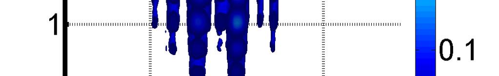
33 To have a short pulse, a broad spectrum is needed. The spectrum has 8 nm width at its base. The theoretical auto-correlation (AC) of the transform-limited (TL) pulse with such spectrum is shown in Fig. 4.(b). As shown in Fig. 3.2, the reference pulse is firstly sent to a dechirp stage (grating pair) and then measured by a homemade auto-correlator. The AC signal is shown in Fig. 4.(c). The full-width-half-maximum (FWHM) of the simulated AC is 69 fs and the FWHM of the measured AC is 83 fs, which indicates the duration of the reference pulse is 54 fs. The discrepancy between the theoretical value and the experimental value might be caused by the residual / introduction of higher order dispersion. But it is clear that most energy is confined in the main lobe of the reference pulse. Compared with the duration of object pulse ( 2 ps), the reference pulse is short enough to be regarded as a δ-function. The object pulse is modulated by a SLM based pulse shaper. A negative group velocity dispersion (GVD) is firstly added to dechirp the pulse. TOD is added as well to generate the Airy pulse. The object pulse and the reference pulse are sent to the cross-correlator. The cross-correslation (XC) signal is shown in Fig. 4.(d). The FWHM of the main lobe of the Airy pulse s XC signal is 7 fs, which corresponding to an intensity duration of 4 fs. A factor of.2244 is used because there is a conversion ratio between the XC signal and the real intensity envelope. The separation between the peak of the main lobe and the peak of the second lobe is 74 fs. From Fig. 4.(d), 9 side lobes which can be clearly recognized from XC. It is evident that the object pulse has an Airy wave form in the time domain D intensity before propagation Using the 3D measurement system based on the configuration in the previous chapter, the Airy- Bessel wave packet is measured in a 3D fashion. The results are shown in Fig The step size of the delay line is 2 µm, corresponding to 4 µm considering the reference go back and forth at the 24

34 (a) Intensity isosurface (b) Sagittal intensity Intensity (a.u.) T (ps) (c) Temporal intensity Figure 4.2: Results of the Airy-Bessel wave packet before propagation. delay line point. So the temporal step size is 3.3 fs. The tilted angle between the object and the reference is.4 rad, which makes the period of interference pattern small but resolvable by the CCD camera. It is worth mentioning that the 3D result is plotted in three different forms. Fig. 4.2(a) plots the data in a isosurface form. The isovalue is chosen to be. the maximum intensity. Fig. 4.2(b) plots the sagittal intensity. The structure of the Airy-Bessel wave packet including the multiple rings of the Bessel beam and the oscillating lobes of the Airy pulse is evident. 8 side lobes can be observed in this form of displaying data. Fig. 4.2(c) sums the transverse intensity to form a D temporal intensity curve. The temporal intensity is plotted in an arbitrary unit scale (the maximum equals to one). The curve has a clear Airy shape. From Fig. 4.2(c), the main lobe has an intensity FWHM of 44 fs, and the separation between the peak of the main lobe and the peak of the second lobe is 87 fs. Recall it that these two values are 4 fs and 74 fs when the same Airy pulse is measured by XC. There is a good agreement between the 3D measurement technique and the conventional method (XC). The main lobe confines the energy of the Airy-Bessel wave packet in a small localized volume (88 µm in diameter, 44 fs in duration), and it is about 7% of the total energy. 25

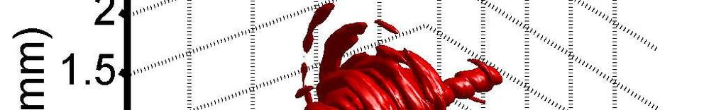
35 (a) Intensity isosurface (b) Sagittal intensity Intensity (a.u.) T (ps) (c) Temporal intensity Figure 4.3: Results of the Airy-Bessel wave packet after propagation D intensity after propagation To observe the evolution of the Airy-Bessel wave packet under the influence of dispersion and diffraction, a 4-inch-long SF glass rod is inserted into the optical path of the object wave packet. The GVD coefficient β 2 of SF is,25 fs 2 /cm. Considering the main lobe pulse duration is 4 fs, a single pass through the dispersive glass rod would correspond to 2 dispersion lengths. The dispersion length, similar with the diffraction length (Rayleigh range), is a parameter to characterize the dispersion effect. It uses the same definition as in Sec To access the 3D measurement system, the delay line at the reference arm has been re-adjusted to ensure the overlap between the object and the reference in the time domain. Using the same measurement parameters in previous case, another 3D measurement is done and the results are shown in Fig The results are plotted in the same fashion as in Fig. 4.2 (isovalue remains. maximum intensity). The FWHM duration of the main lobe was 34 fs. In the time domain, the Airy pulse can keep its shape against dispersion. It is also apparent that the wave packet s intensity profile has not significantly changed. In previous measurement, the distance from the axicon to the camera is 4 cm, which is 7 diffraction lengths (Rayleigh range). The extra optical path 26

36 8 5 φ(t)/π (rad) φ(t)/π (rad) Time (ps).5.5 Time (ps) (a) Temporal phase before propagation (b) Temporal phase after propagation Figure 4.4: Temporal phase results for Airy-Bessel wave packet. provided by the glass rod was 3.23 diffraction lengths, so 2 diffraction lengths in total. After such dispersion and diffraction effect added, the main lobe (86 µm in diameter, 34 fs in duration) still consists 7.57% of the total energy. It is obvious that he peak power of the Airy-Bessel wave packet is conserved by comparing two measurement results of the Airy-Bessel wave packet before and after propagation Temporal phase retrieval The temporal phase of the Airy-Bessel wave packet is also retrievable from the data of the 3D measurement. Assumption that the reference beam and the object beam has no phase variation within a small regime is valid for the Airy-Bessel case. The temporal phase before and after propagation through the glass rod are plotted in Fig. 4.4 respectively. φ(t) is displayed in the scale of π. From Fig. 4.4(a), the Airy pulse signature is evident from the π phase shift between each lobes. After the Airy-Bessel wave packet propagates through the dispersive glass (4-inch-long SF), the π phase shift gets blurred as shown in Fig. 4.4(b), which is a result from extra dispersion effect added. If 27

37 Intensity (a.u.) Wavelength (nm) (a) Laser spectrum Simulated AC (a.u.) Delay (fs) (b) Simulated AC Measured AC(a.u.) Delay(fs) (c) Measured AC XC signal(a.u.) Delay(fs) (d) Measured XC Figure 4.5: Experimental parameters for Airy-Airy-Airy measurements. more dispersion effect is added, finally the pulse evolution will get dominated by GVD and the temporal phase will have a parabolic shape. 4.2 Measurement of Airy-Airy-Airy wave packet Due to their self-acceleration, self-healing and lateral acceleration properties, Airy beams and Airy pulses have been studied in many researches [2, 5, 7, 23]. An Airy-Airy-Airy wave packet (AAA) has an Airy wave form in all three dimensions (Cartesian coordinate system), x,y and t. The spatial profile of AAA is a 2D Airy beam and the temporal profile is an Airy pulse. Since the Airy wave is the only D wave that can propagation without distortion, AAA can propagation without dispersion or diffraction as well. It means an AAA belongs to the family of linear light bullet s. Daryoush et al. has studied the AAA both in linear and nonlinear regime [2]. In the following portion of this section, the AAA will be measured in 3D. The experimental setup is same as the sketch in Fig The object beam is expanded by a factor of 3 using a telescope configuration. Then it goes through a SLM based beam shaper. The phase added on the object beam is same as what is suggested in [5]. The laser spectrum, TL AC signal, experimental AC signal and XC signal are shown in Fig. 4.5 respectively. The laser spectrum, centered at 3 nm, has 65 nm width at its base. The simulated TL AC has a FWHM of 89 fs. 28

38 (a) Intensity isosurface (b) Sagittal intensity Intensity (a.u.) T (ps) (c) Temporal intensity Figure 4.6: Results of the Airy-Airy-Airy wave packet. Measured AC has a FWHM of 3 fs. The higher order dispersion left on the reference pulse is acceptable since the reference pulse is considerably shorter than the object pulse. Fig. 4.5(d) shows the XC signal between the object pulse and the reference pulse, revealing a clear Airy pulse shape. The object pulse duration is 2 ps so that the δ-function assumption is valid. The 3D measurement uses almost the same experimental parameters in previous Airy-Bessel section, except the tilted angle between the object wave packet and the reference wave packet is.56 rad. The measurement results are shown in Fig From Fig. 4.6(a), the AAA structure has been nicely retrieved by this 3D measurement technique with Airy function distribution in all x, y and t directions. The sagittal plotting (Fig. 4.6(b)) shows clear 2D Airy profile in y-t plane. And the D temporal intensity (Fig. 4.6(c)) agrees well with XC signals. Meanwhile, based on the data collected, the temporal phase of an AAA can be retrieved. The result is shown in Fig The temporal phase φ(t) is plotted in the scale of π. The Airy pulse has a π phase shift signature, which is evident from the measurement result. 29

39 φ(t)/π (rad) Time (ps) Figure 4.7: Temporal phase retrieval of Airy-Airy-Airy wave packet. 4.3 Measurement of dual-airy-airy-rings wave packet An Airy-Airy-Airy wave packet has an Airy distribution in all three dimensions of a Cartesian coordinate system. If the coordinate system is converted into a cylindrical coordinate system, Airy rings can be generated if there is an Airy distribution in the radial direction. Nikolaos et al. pointed it out that such radial wave can have abruptly autofocusing property []. Later on their group managed to generate such radially symmetric Airy beam [2]. It has been proposed that superposed with two facing Airy pulses in the time domain, such wave packet can have 3D autofocusing. In the following portion of this section, a dual-airy-airy-rings wave packet (daar) has been experimentally generated and measured in 3D. Its 3D autofocusing effect has also been observed. The experimental parameters can be found in Fig The laser spectrum has 8 nm at its base. The simulated AC FWHM is 62 fs. The experimental AC FWHM is 83 fs, corresponding to a pulse duration of 54 fs. Using the same phase pattern as suggested in Sec. 2..2, dual Airy pulses can be generated. Fig. 4.8(d) shows the experimental XC signal of two Airy pulses. Under the influence of normal 3

40 Intensity (a.u.) Wavelength (nm) (a) Laser spectrum Simulated AC (a.u.) Delay (fs) (b) Simulated AC Measured AC(a.u.) Delay(fs) (c) Measured AC XC signal(a.u.) Delay(fs) (d) Measured XC Figure 4.8: Experimental parameters for dual-airy-airy-rings measurements. dispersion, these two Airy pulses will accelerate to the center. In other words, they will collapse (counter propagate and form a higher peak intensity) in the time domain under normal dispersion. This effect can be also checked by applying normal GVD at the pulse shaper. The separation between two Airy waves peak can be adjusted by varying the amount of triangle phase. The delay in the time domain depends on the amount of linear phase in the spectrum (frequency) domain. To observe the real autofocusing effect, the glass rod (4-inch-long SF) has been put into the optical path of the dual Airy pulses. The linear phase is adjusted so that in the XC signal a highest peak is formed. When the glass rod is removed, the temporal profile becomes dual Airy pulses with a modified separation between two peaks. Using the configuration shown in Fig. 3.3, Airy rings can be generated at the Fourier plane (back focal plane of the Fourier lens). The 3D measurement results of daar at the Fourier plane are shown in Fig Fig. 4.9(c) gives the D temporal intensity. Compared with the previous XC signals, the separation between two peaks is smaller. Then the glass rod is re-inserted into the object arm. The CCD camera is moved 2 cm away from the Fourier plane. At that position, tightly focused beam can be observed. Another 3D measurement is done and the results are shown in Fig. 4.. It is evident that the daar can autofocus in 3

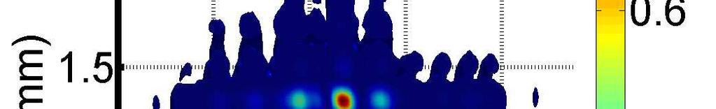
41 (a) Intensity isosurface (b) Sagittal intensity Intensity (a.u.) T (ps) (c) Temporal intensity Figure 4.9: Results of the dual-airy-airy-rings wave packet at the Fourier plane. Intensity (a.u.) (a) Intensity isosurface (b) Sagittal intensity T (ps) (c) Temporal intensity Figure 4.: Results of the dual-airy-airy-rings wave packet at the autofocus plane. 32