A Study in the Prediction of Residual Stresses in Shot Peening

Transcription

1 A Study in the Prediction of Residual Stresses in Shot Peening By Robert Howard A Thesis Submitted to the Graduate Faculty of Rensselaer Polytechnic Institute in Partial Fulfillment of the Requirements for the degree of MASTER OF SCIENCE IN MECHANICAL ENGINEERING Approved: Dr. Ernesto Gutierrez-Miravete, Thesis Advisor Rensselaer Polytechnic Institute Hartford, Connecticut September, 008

2 Copyright 008 by Robert G. Howard All Rights Reserved ii

3 CONTENTS LIST OF TABLES LIST OF FIGURES.. LIST OF EQUATIONS NOMENCLATURE.. ACKNOWLEDGMENT... ABSTRACT Introduction Residual Stress. 1.. Shot Peening Introduction Almen Intensity Shot Peening Induced Residual Stress Measurement of Residual Strains Using X-Ray Diffraction 1.3. Fatigue Introduction Stress Relaxation During Fatigue Loading Modeling of Shot Peening Processes Brief Historical Background.. Materials...1. Ti-6Al-4V.1.1. Introduction Johnson-Cook Material Model.... Shot Material 3. Methodology of Analysis 3.1. Mathematical Formulation of Shot Peening Problem Introduction Governing Equations in Polar Coordinates Governing Equations in Cartesian Coordinates FEM Formulation.. vi viii xiv xvii xix xx iii

4 3.. D Axisymmetric Analysis Model Setup D Cartesian Analysis with Uniform Shot Spacing Model Setup D Cartesian Analysis with Random Shot Spacing Model Setup.. 4. Results and Discussion 4.1. D Axisymmetric Analysis Introduction Steel Shot Surface Displacement Data Stress Data Glass Shot Surface Displacement Data Stress Data. 4.. D Cartesian Analysis with Uniform Shot Spacing Introduction Steel Shot Surface Displacement Data Stress Data Glass Shot Surface Displacement Data Stress Data D Cartesian Analysis with Random Shot Spacing Introduction Steel Shot Surface Displacement Data Stress Data Glass Shot Surface Displacement Data iv

5 Stress Data Conclusions Introduction D Axisymmetric Analysis D Cartesian Analysis with Uniform Shot Spacing 5.4. D Cartesian Analysis with Random Shot Spacing General. REFERENCES.. APPENDIX A: D Axisymmetric ABAQUS Models. APPENDIX B: D Axisymmetric Stress Contour Plots (Steel Shot).. APPENDIX C: D Axisymmetric Stress Contour Plots (Glass Shot). APPENDIX D: D Cartesian ABAQUS Models with Uniform Shot Spacing... APPENDIX E: D Cartesian Stress Contour Plots (Uniformly Spaced Steel Shot)... APPENDIX F: D Cartesian Stress Contour Plots (Uniformly Spaced Glass Shot)... APPENDIX G: D Cartesian ABAQUS Models with Random Shot Spacing APPENDIX H: D Cartesian Stress Contour Plots (Randomly Spaced Steel Shot)... APPENDIX J: D Cartesian Stress Contour Plots (Randomly Spaced Glass Shot)... APPENDIX K: ABAQUS Validation Studies v

6 LIST OF TABLES Table 1.1 Table 1. Table.1 Table. Table 3.1 Table 3. Table 3.3 Table 3.4 Table 3.5 Table 4.1 Table 4. Table 4.3 Table 4.4 Table 4.5 Table 4.6 Table K1 Table K Table K3 Table K4 Table K5 Table K6 Table K7 Table K8 Table K9 Table K10.. Table K11.. Table K1.. Table K13.. Table K14.. Table K vi

7 Table K16.. Table K17.. Table K18.. Table K19.. Table K0.. Table K1.. Table K.. Table K3.. Table K4.. Table K5.. Table K6.. Table K vii

8 LIST OF FIGURES Figure Figure 1... Figure Figure Figure Figure.1.. Figure Figure 3... Figure Figure Figure Figure Figure Figure Figure Figure 3.10 Figure 3.11 Figure 3.1 Figure Figure 4... Figure Figure Figure Figure Figure Figure Figure Figure 4.10 Figure 4.11 Figure viii

9 Figure 4.13 Figure 4.14 Figure 4.15 Figure 4.16 Figure 4.17 Figure 4.18 Figure 4.19 Figure 4.0 Figure 4.1 Figure 4. Figure 4.3 Figure 4.4 Figure 4.5 Figure 4.6 Figure 4.7 Figure 4.8 Figure 4.9 Figure 4.30 Figure 4.31 Figure 4.3 Figure 4.33 Figure 4.34 Figure 4.35 Figure 4.36 Figure 4.37 Figure 4.38 Figure 4.39 Figure 4.40 Figure 4.41 Figure A1.. Figure A ix

10 Figure A3.. Figure A4.. Figure B1.. Figure B.. Figure B3.. Figure B4.. Figure B5.. Figure B6.. Figure B7.. Figure B8.. Figure C1.. Figure C.. Figure C3.. Figure C4.. Figure C5.. Figure C6.. Figure C7.. Figure C8.. Figure D1.. Figure D.. Figure D3.. Figure E1.. Figure E.. Figure E3.. Figure E4.. Figure E5.. Figure E6.. Figure F1.. Figure F.. Figure F3.. Figure F x

11 Figure F5.. Figure F6.. Figure G1.. Figure G.. Figure H1.. Figure H.. Figure H3.. Figure H4.. Figure H5.. Figure H6.. Figure H7.. Figure H8.. Figure J1 Figure J Figure J3 Figure J4 Figure J5 Figure J6 Figure J7 Figure J8 Figure K1.. Figure K.. Figure K3.. Figure K4.. Figure K5.. Figure K6.. Figure K7.. Figure K8.. Figure K9.. Figure K10 Figure K xi

12 Figure K1 Figure K13 Figure K14 Figure K15 Figure K16 Figure K17 Figure K18 Figure K19 Figure K0 Figure K1 Figure K Figure K3 Figure K4 Figure K5 Figure K6 Figure K7 Figure K8 Figure K9 Figure K30 Figure K31 Figure K3 Figure K33 Figure K34 Figure K35 Figure K36 Figure K37 Figure K38 Figure K39 Figure K40 Figure K41 Figure K xii

13 Figure K43 Figure K44 Figure K45 Figure K46 Figure K47 Figure K48 Figure K49 Figure K50 Figure K51 Figure K5 Figure K53 Figure K54 Figure K55 Figure K56 Figure K57 Figure K58 Figure K xiii

14 LIST OF EQUATIONS Equation Equation 1... Equation Equation Equation Equation Equation Equation Equation Equation 1.10 Equation 1.11 Equation 1.1 Equation.1.. Equation... Equation Equation 3... Equation Equation Equation Equation Equation Equation Equation Equation 3.10 Equation 3.11 Equation 3.1 Equation 3.13 Equation 3.14 Equation 3.15 Equation xiv

15 Equation 3.17 Equation 3.18 Equation 3.19 Equation 3.0 Equation 3.1 Equation 3. Equation 3.3 Equation 3.4 Equation 3.5 Equation 3.6 Equation 3.7 Equation 3.8 Equation 3.9 Equation 3.30 Equation 3.31 Equation 3.3 Equation 3.33 Equation 3.34 Equation 3.35 Equation 3.36 Equation 3.37 Equation 3.38 Equation 3.39 Equation 3.40 Equation 3.41 Equation 3.4 Equation 3.43 Equation 3.44 Equation 3.45 Equation K1.. Equation K xv

16 Equation K3.. Equation K4.. Equation K5.. Equation K6.. Equation K7.. Equation K8.. Equation K9.. Equation K10 Equation K11 Equation K1 Equation K xvi

17 NOMENCLATURE NOTE: Nomenclature applies strictly to Section 3.1: Mathematical Formulation of Shot Peening Problem. Nomenclature in all other sections is clearly defined within those sections. Subscript Description r r-direction θ θ-direction x x-direction y y-direction z z-direction 0 Initial condition 1 Body #1 (disk or plate) Body # (shot) Symbol Units Description a m Radius of the surface of contact α m Displacement β N A matrix that depends on the current position of the material point being considered δd m/s The symmetric component of the virtual velocity gradient E N/m, Pa Modulus of elasticity ε Normal strain F N/m 3 Body force f N/m 3 Body force at any point within the volume, V G N/m, Pa Shear modulus γ Shear strain K N/m, Pa Bulk modulus k m /N, 1/Pa Material constant, k 1 ν = πe xvii

18 N N P N Load φ radians Rotation Interpolation functions that depend on some material coordinate system q max N/m, Pa Maximum pressure load R m Radius r m Radius ρ kg/m 3 Density S m Surface bounding volume, V σ N/m, Pa Normal stress t N/m Surface traction at any point on S τ N/m, Pa Shear stress τ c u m Displacement Any conjugate pairing of material stress measures V m 3 Volume occupied by a part of the body in the current configuration v m/s Velocity ν Poisson s ratio δv m/s A virtual velocity field z m Depth xviii

19 ACKNOWLEDGEMENT I would like to thank Dr. Ernesto Gutierrez-Miravete for his continuous guidance and support throughout this thesis. Also, without the encouragement and support of my friends and family I would not have been able to complete this project. Thanks. xix

20 ABSTRACT Of significant importance to the design of aerospace and automobile components is the fatigue life of these components when subjected to variable loading conditions. Research has shown that the fatigue life of a component can be significantly improved through the use of shot peening. Because of this there is a need to develop numerical models that are capable of accurately predicting residual stresses produced from peening operations. This thesis presents a mathematical model and its computer implementation of the shot peening process. The finite element method was employed to study the elastic-plastic dynamic process of shots impacting a metallic target. The target material modeled was Ti-6Al-4V. Through the use of the Johnson-Cook flow stress model Ti- 6Al-4V was modeled as a rate sensitive material. Rigid models for the shot were created in which both steel and glass shot materials were interchanged. Analysis was carried out using both axisymmetric and Cartesian models. Situations of single and multiple shot impacts were studied. The models developed were employed to determine the effects that multiple shot impacts have on the residual stress profiles created on and beneath the surface of the target. Specifically of interest was the magnitude of the residual stress on the surface, as well as the magnitude of the maximum compressive residual stress developed beneath the surface of the target. Other values of interest included the depth of the compressive layer and the magnitude of the maximum tensile residual stress. Results show that the predicted residual stress profiles follow the same trends as those acquired from published experimental results, as well as, finite element modeling of peening processes by past researchers. xx

21 1. INTRODUCTION Titanium has become a prominent material in many industries including aerospace, automotive, biomedical, and many more owing to its above average strength to weight ratio. Titanium alloys are currently being used to construct everything from bike frames and tennis rackets to airframes and automotive components. The most widely used titanium alloy is Ti-6Al-4V or Ti64 as it is commonly called, which accounts for 45% of total titanium production and can found in all of the aforementioned industries [1]. As the name suggests this alloy is comprised of 6-wt% aluminum and 4-wt% vanadium. Due to its wide usage it is important that as much information as possible be gathered about this particular alpha-beta alloy, and in particular the effects that the various processing techniques have on the final properties of the material. While one can easily open a book and obtain the basic mechanical properties of Ti64 (i.e. yield strength, young s modulus, and fatigue life) these are often representative of the preprocessed alloy. Actual mechanical properties of a component made from Ti64 can vary greatly depending on the manufacturing processes used to produce the component such as finish machining, shot peening and heat treatment. For this reason it is important to study the impact that these manufacturing processes have on the mechanical properties of the material. Titanium is a material generally utilized for parts requiring the greatest reliability and therefore the surface roughness, and any damage to the sub-surface layers (including residual stress) must be controlled []. The main focus of this research will be the residual stresses formed during shot peening of Ti-6Al-4V. 1.1 Residual Stress The primary focus of this research is to estimate the residual stresses resulting from shot peening Ti-6Al-4V. It is necessary to first present a brief background on such subjects as residual stress, shot peening, and fatigue. In this section a brief description of what residual stresses are and how they are introduced will be presented. Residual stresses are one of the most important parameters that characterize the near surface layer of any mechanical component, which plays a crucial role in controlling its performance [3]. A residual stress is one that remains in a body even when all external loads have been removed and is the result of a non-uniform plastic deformation. Such stresses are 1

22 generally the result of a previous thermal or mechanical load applied to the body or of a phase transformation that occurs within the body itself [3]. An example of a thermal load would be one that is applied during a heat treatment process, while mechanical loading can occur during finish machining, bending, or shot peening operations. 1. Shot Peening 1..1 Introduction This section provides a brief description of the shot peening operation including the many parameters that are involved. Information is also provided regarding the measurement of peening intensities, as well as, the role that shot peening plays in the formation of residual stresses in the peened component. Shot peening is a surface strain hardening process that is used mainly in the manufacture of mechanical components [4, 5]. Strain hardening can be described as a process in which a ductile metal will become harder and stronger as it is plastically deformed. This process is also referred to as work hardening or cold working since the temperature at which it usually takes place is well below the absolute melting temperature of the material being worked on. In order to explain the fundamental principle behind strain hardening one must look at the dislocation-dislocation strain field interactions. Cold working causes the dislocation density in the material to increase resulting in a decrease in the average distance between the dislocations. The movement of a dislocation is hampered by the presence of other dislocations because of the repulsive interaction that occurs between them. As a result the stress required to further deform the ductile metal increases [4]. Overall, shot peening has been proven to markedly improve the fatigue life of a component. This is accomplished by impinging the surface of the component with many small spherical shots. Typical shot materials include hardened cast-steel, conditioned cut-wire, glass, or ceramic beads. Shot velocities can range from 40m/s to 70m/s. The size of the beads can vary from 0.1mm to mm in diameter [5]. After contact between the shot and the target material has ceased, the elastically stressed region tends to recover to the fully unloaded state, while the plastically deformed region sustains some permanent deformation [6]. The final result is a target material that contains

23 compressive stresses in the uppermost layer with tensile stresses present in the layers beneath the surface [6]. One of the main problems related to the shot peening process are the many operating parameters that are involved. These include shot speed, dimensions, shape, nature and hardness of the shot, projection angle, exposure time, and coverage. Controlling shot peening operations with any sort of repeatability is made extremely difficult due to this multitude of parameters [5]. 1.. Almen Intensity The Almen test is the method by which the shot peening process is typically controlled and measured and is a gauge of its intensity. In general Almen tests are carried out in accordance with the United State Military Standard MILS-13165B [7]. During the test, a metal strip is fastened to a block and then subjected to a shot peening operation. Upon removal from the block the metal strip will tend to arc in the direction of the shot peened face. The intensity of the shot peening operation is then judged by the height of the arc and can be measured using an Almen gauge [7]. Depending on the intensity of the shot peening operation there exist several different types of Almen strips. Almen strips having an A, C, or N designation are the most commonly used of the group. These are shot peened to a condition defined as saturation when doubling the exposure time of the strip to the shot peening will produce less than a 10 per cent increase in arc height [7]. The name Almen intensity, however, can be slightly deceiving as it is not necessarily a measure of the intensity of the shot peening process but more a measure of the deformation caused by a particular shot peening intensity. Typical designations for Almen intensity will quote the arc height or a multiple of the arc height followed by a letter signifying the type of Almen strip that was used [7]. Given two components that are shot peened to the same Almen intensity it is possible for different depths of plastically deformed material and residual stress distributions to be obtained. Because of this it is not possible to associate a particular Almen number with a certain quantifiable fatigue benefit [7]. However, research has been done to try to associate Almen intensity to residual stresses induced by shot peening. In his work, Guagliano [8] found that for a defined 3

24 shot type (i.e. size and material) the Almen intensity could be directly related to the component of shot velocity perpendicular to the target being peened. He developed a series of equations for various shot diameters of steel or ceramic shot in which he expressed the Almen intensity as a function of the shot velocity. At the conclusion of his work Guagliano stated that analytical functions relating Almen intensity to shot velocity were found for the shot considered: the best-fitting equations were found and the regression coefficient is always good. It is thus possible to relate the residual stresses in a mechanical part to Almen intensity [8] Shot Peening Induced Residual Stress Given the nature of the shot peening operation it can be concluded that the bulk of the residual stresses produced from this process are the result of mechanical loading. The constant bombardment of the target material results in compressive residual stresses on the surface layer and tensile residual stresses throughout the bulk of the sub-surface material. Figure 1.1 shows a typical residual stress profile following a peening operation. As one can see, the residual stress profile indicates a compressive stress at the surface of the component and a tensile stress throughout the remaining bulk of the component. Figure 1.1: Shown here is a typical residual stress profile that would result from a peening operation. Shown in Figure 1. is a schematic diagram depicting the beneficial effects that shot peening has for both axial loading and bending conditions [7]. The residual stress profile 4

25 shown in this figure for both the axial loading and bending conditions is representative of one that would result following a shot peening operation. After the application of an applied tensile load or bending moment the resultant stress profile is given. In this case the stresses at the surface of the component remain compressive. However, in a more general sense, the presence of the surface compressive residual stress cancels out part the applied stress so that the resultant stress is less than it would normally be had no residual stresses been present. It is precisely this effect that can have a profound impact on the fatigue life of the material. Figure 1.: Interaction of applied and residual stress during (a) tensile loading and (b) bending [7]. 5

26 1..4 Measurement of Residual Strains Using X-Ray Diffraction X-ray diffraction is the most commonly used method of experimentally obtaining residual stress data from shot peened components. X-ray diffraction can be utilized for either macroscopic stress or microscopic stress measurement. Macrocopic stress measurements, such as residual stress, are those measurements, which extend over a distance that is relatively large when compared to the grain size of the material. Macroscopic stresses are generally of greater interest as they tend to be the ones more closely associated with design and failure analysis [9]. So how are residual stresses measured using x-ray diffraction? They are not. Stress, because it is an extrinsic property, is not measurable; however, strain can be measured. X-ray diffraction therefore measures the strain in the crystal lattice of the material and the associated residual stress is then calculated based on the measured strain. During x-ray diffraction only elastic strains in the crystal lattice are measured. Strains that exceed the elastic limit of the material cause dislocation motion, which disrupt the lattice structure and result in the formation of microstresses, but they do not affect the residual macrostresses as following deformation these remain primarily elastic [9]. Figure 1.3 and Figure 1.4 show the diffraction, at a high diffraction angle, θ, from the surface of a monochromatic beam of x-rays. Note that a tensile stress, σ, is being applied parallel to the sample surface. In this case the angle, ψ, represents the orientation of the sample surface and is defined as the angle between the normal of the surface and the incident and diffracted beam bisector [9]. X-ray beam diffraction occurs at an angle θ where θ is defined by Bragg s Law. n λ = d sinθ (1.1) Where n = an integer denoting the order if diffraction λ = the x-ray wavelength d = lattice spacing of the crystal planes θ = the diffraction angle 6

27 In the above equation n and λ are known quantities. Therefore any change in the lattice spacing, d, will result in a change in the diffraction angle, θ [9]. Figure 1.3 shows the sample in the ψ = 0 orientation. The lattice spacing, d, in this orientation is reduced due to the Poisson s ratio contraction that is a byproduct of the tensile stress acting parallel to the surface. Figure 1.4 shows the same sample surface depicted in Figure 1.3 except now it has been rotated through a known angle ψ = ψ. Due to the orientation of the surface shown in Figure 1.3 the applied tensile stress causes the lattice spacing to increase. This results in a subsequent decrease in the diffraction angle, θ. Having obtained the angular position of the diffraction peak for two orientations of the sample surface, ψ = 0 and ψ = ψ, it becomes possible to calculate the stress in the plane of diffraction on the sample surface [9]. Figure 1.3: Shown above is the sample surface in the ψ =0 orientation. [9] Figure 1.4: Shown here is the same sample surface as in Figure 1.3 except rotated through a known angle ψ = ψ. [9] NOTE: D = x-ray detector, S = x-ray source, and N = normal to surface In order to calculate residual stress using x-ray diffraction one must determine the arithmetic average stress in a volume of material that is bounded by the depth of penetration of the x-ray beam and the irradiated area [9]. Given in Table 1.1 are the 7

28 recommended diffraction parameters for Ti-6Al-4V. The value of K 45 represents the relative sensitivity and is defined as the magnitude of the stress necessary to cause an apparent shift in diffraction-peak position of 1 for a 45 ψ tilt [9]. As K 45 increases the sensitivity of the measurement decreases [0]. In determining residual stresses from x-ray diffraction the plane-stress elastic model is the one most commonly used. Here, measurement is restricted to the surface of the sample only and thus for subsurface measurements electropolishing must be used. As the name implies a condition of plane stress, σ 3 = 0, is assumed for the surface of the material being measured [9]. Shown in Figure 1.5 is the plane-stress model that is used to determine residual stress based on the elastic strain measurement obtained by x-ray diffraction [9]. Figure 1.5: Shown here is the plane-stress model used to calculate residual stress from strain measurements obtained by utilizing x-ray diffraction. [9] 8

29 Table 1.1: X-ray diffraction techniques for the measurement of residual stresses in Ti-6Al-4V. [9] Alloy Radiation Lattice Angle, Elastic Constants Bulk K45 Linear Absorption Plane θ (E/1+ν) Error Coefficient (µ) (hkl) Bulk (hkl) (deg) GPa % MPa cm -1 Ti-6Al-4V CuKα (1.3) ±

30 The following derivation shows how values of residual stress are calculated based on the measurement of elastic strain data using x-ray diffraction techniques. The strain, ε φψ, is given by [9]. 1+ ν E ν ( σ α + σ α ) ( σ + σ ) ε φψ = E (1.) Where E = Elastic Modulus ν = Poisson s Ratio α 1 and α = Angle Cosines of the Strain Vector σ 1 and σ = Principle Stresses and α1 = cosφ sinψ (1.3) α = sinφ sinψ (1.4) By substituting the angle cosines into Equation 1. and performing some minor simplification it is then possible to express the strain in terms of the orientation angles as follows. ε 1+ ν ν σ φ sin ψ E E ( σ + σ ) φψ = 1 (1.5) Where ( σ cos φ) + ( σ φ) = 1 sin (1.6) σ φ For the orientation angle, ψ, if ψ = 90 the strain vector lies in the same plane as the 10

31 surface being measured. Equation 1.5 relates the surface stress, σ φ, in any direction defined by the angle ψ, to the strain, ε, in the direction (φ, ψ) and the principal stresses in the surface [9]. This strain can also be expressed in terms of changes in the linear dimensions of the crystal lattice. d dφψ d 0 ε φψ = = (1.7) d 0 d 0 Where d φψ = Spacing between the lattice planes measured in the direction defined by φ and ψ. d 0 = Stress-free Lattice Spacing Substituting Equation 1.7 into Equation 1.5 yields the following. d φψ d d ν = E σ sin ν ψ φ ( hkl ) E ( hkl ) ( σ + σ ) 1 (1.8) Which can be used to determine the lattice spacing in any direction. The above equation describes the fundamental relationship between lattice spacing and the biaxial stresses in the surface of the sample, and shows that the lattice spacing is a linear function of sin ψ. The slope and intercept are given by Equation 1.9 and 1.10 respectively. dφψ 1+ ν = sin ψ E ( hkl ) σ d φ 0 (1.9) ν ν d φ 0 = d 0 d 0 ( σ 1 + σ ) = d 0 1 ( σ 1 + σ ) (1.10) E ( hkl ) E ( hkl ) 11

32 Solving the equation for the slope for the stress σ φ yields. σ E 1 d φψ φ = + 1 ν ( hkl ) d 0 sin ψ (1.11) Because the value of d φ0 differs from d 0 by not even ±1% it is possible to approximate σ φ to this same accuracy using Equation 1.1 below. σ E d φψ = φ 1+ ν ( ) φ hkl d 0 sin 1 ψ (1.1) In general there are three common techniques used for x-ray diffraction that take advantage of the plane-stress elastic model. These techniques are single-angle, two angle, and sin ψ. The two-angle technique is the one most commonly used in the United States and has been thoroughly vetted by the Society of Automotive Engineers (SAE). All of the techniques mentioned are founded on the relationship between lattice spacing and stress that was given in Equation 1.1 above [9]. X-ray diffraction has its limitations. The apparatus needed to perform x-ray diffraction is expensive and delicate. This tends to limit the use of x-ray diffraction to laboratories. Because all of the techniques listed previously only measure stress on a surface, the use of electropolishing is necessary when residual stress data in the subsurface layers is needed. Electropolishing is preferred because no residual stresses are induced, and if properly performed, preferential etching of the grain boundaries does not occur [9]. Other mechanical methods of layer removal deform the surface and induce residual stress [9]. The use of x-ray diffraction also requires that the material be polycrystalline and posses a fine grain size. Finally, the time required to complete a single residual stress measurement can be as much as 1 hour when material removal and sample repositioning are accounted for [9]. 1

33 1.3 Fatigue Introduction Now that both a brief description of residual stress and a background of shot peening have been given it is time to discuss fatigue and the effect that shot peening has on the overall fatigue life of a mechanical component. According to Callister [4], fatigue can be defined as failure, at relatively low stress levels, of structures that are subjected to fluctuating and cyclic stresses. Under such cyclical loading conditions components have a tendency to fail at stress magnitudes that are well below the material s understood tensile or yield strength for static loading conditions. As the name itself implies fatigue failures tend to occur over a rather lengthy period of time. As the driving factor behind approximately 90% of all metallic failures, fatigue is the single largest cause of failure in metals. Because very little plastic deformation is associated with fatigue failure it tends to be brittle by nature and is brought on by the generation and propagation of cracks through the material. At the same time, because of its more brittle nature, fatigue can occur suddenly and without warning, which results in catastrophic failure [4]. In general there are three key parameters that can be used to describe the fatigue characteristics of a material. These are the fatigue limit, fatigue life, and fatigue strength. The fatigue limit is the maximum stress level below which a material can endure an essentially infinite number of stress cycles and not fail. The fatigue life of a material is the total number of stress cycles that will cause a fatigue failure at some specified stress amplitude. Finally, the fatigue strength refers to the maximum stress level that a material can sustain, without failing, for some specified number of cycles [4]. It is widely accepted that compressive residual stresses improve the overall fatigue life of a component, however, what is not known is the exact impact that these stresses have [10]. Amongst researchers there seems to be an increased interest in developing models capable of incorporating residual stress values into fatigue life calculations [10]. The difficulties in controlling the parameters of the strain hardening operation by shot peening very often lead its users to treat it only as an extra safety factor, without taking the residual stresses due to the shot peening into account when calculating the required dimensions of the part [5]. In the United States and France component developers tend to follow the previously stated approach, however, in England, Germany, China, and 13

34 Japan engineers take residual stresses due to shot peening, in the stabilized condition, into account in their fatigue life calculations [5]. At the present time controversy exists in the shot peening and fatigue community as to whether the major benefits of shot peening should be ascribed to the compressive residual stresses or to the microstructural changes and/or deformation which occur over the same region and influence crack initiation [10]. Niku-Lari found that for materials which posses low characteristics the resulting increase in the endurance limit due to the shot peening operation is primarily caused by the superficial strain hardening and the residual stresses while for high strength materials the increase in fatigue life has been found to be caused by the residual stresses [5]. Shown in Table 1. below are some practical examples of how shot peening has impacted the overall fatigue life of several different types of components ranging from pins to tank tracks [5]. Table 1.: Practical applications of shot peening improving fatigue life [5]. Type of Part Applied Stress Increase in Service Life (%) Pins Alternate Bending Shafts Torsion 700 Gearbox Shafts Service Life Tests 80 Crankshafts Service Life Tests 300 but very variable Aircraft Link Rods Push/Pull 105 Connecting Rods Push/Pull 45 Leaf Springs Dynamic Stress Helical Springs Service Life 3500 Torsion Bars Dynamic Stress Cardan Coupling Shafts Alternate Bending 350 Gears Service Life Tests 130 Tanks Tracks Service Life Tests 1100 Weldments Service Life Tests 00 Valves Service Life Tests 700 Rocker Arms Service Life Tests 30 14

35 1.3. Stress Relaxation During Fatigue Loading Several prominent researchers have discovered that the magnitudes and distributions of the residual stresses change during fatigue loading [5,10]. This is one of the main reasons why accounting for the residual stresses developed during peening operations in fatigue life calculations becomes very difficult. General practice dictates that engineers are only allowed to account for the values of stabilized stresses. A stabilized stress is one that is present in a component for the majority of its operating life [5]. In his work James [10] studied the relaxation of residual stresses during fatigue loading of 7050-T7451. He found that for peak cyclic stress of only ~43% of the proof stress, tensile strains in the ST direction at <0.5% of the life (10,000 cycles) had relaxed by around 5% from the peak value, and this reduction remains fairly constant up to 5% of life (100,000 cycles) [10]. At the same time James concluded that a consistent trend through the depth of the specimen for the compressive strains parallel to the surface did not exist. He found for the majority of data analyzed that there was an approximate 5% reduction in the compressive strain due to relaxation during fatigue loading [10]. 1.4 Modeling of Shot Peening Processes Brief Historical Background At the present time, the only methods that exist for the direct measurement of residual stresses formed during shot peening are through the use of semi-destructive methods, such as X-ray diffraction, which can be time consuming and very expensive to undertake [6]. Another drawback to current methods of measuring residual stresses is that they do not lend themselves to the examination of the effect of key shot peening parameters on the residual stress profiles generated [11]. Therefore modeling of the shot peening process [can be] of considerable significance to the understanding of the process and of the parameters, which govern its performance [6]. Over the years several studies have been performed in order to determine the most effective method for simulating shot peening. While the majority of them focus around the use of numerical finite element methods a few have explored other means by which to simulate peening operations. Slim [1] simulated the effect of shot peening on a volume element through the use of uniaxial strain controlled cyclic loading. He hypothesized that if the change in 15

36 material properties due to this type of loading could be determined, that the data, in conjunction with the shot peening parameters, could be used to predict the residual stress profile [1]. He found that it is possible to use the curve of cyclic hardening obtained from a uniaxial tension/compression test to model material behavior and to then use the parameters obtained to predict the residual stress profile that would be created from shot peening the material. This conclusion is primarily based on the fact that the shapes of the deviatoric stress for shot peening and tension/compression are very similar [1]. It is important to note that Slim only used the uniaxial tension/compression test to determine the material properties. Residual stress data was then calculated using a proprietary code called PEENSTRESS developed by ENSAM and the Metal Improvement Company [1]. Over the past several years a multitude of numerical finite element models have been developed for the purpose of simulating shot peening operations. During the early stages of his research in simulating shot peening operations using finite element programs Meguid [13,14] developed models involving single and double impingement [13, 14]. During his simulations he sought to determine the effect that the various peening parameters (i.e. shot velocity, size, and shape) have on the resulting residual stress profiles. For the development of his model he chose to use the ANSYS finite element analysis package [13]. For the single impingement case Meguid concluded that although shot velocity does affect the surface compressive residual stresses it has an insignificant effect on the maximum sub-surface residual stress values. Meguid also found that with increasing shot size the depth of the compressed layer increased [13]. Similar results were obtained for his double impingement model in which he simulated two shots contacting the target simultaneously [14]. From his research Meguid concluded that the shot velocity, shot shape, and the separation distance between shots has an effect on the depth of the compressed layer, as well as, the magnitudes of the surface and sub-surface residual stresses [14]. Moving forward from the single and double impingement models Meguid went on to develop a finite element model to simulate the impingement of multiple shots on a AISI 4340 steel target, which he modeled as a strain rate sensitive material [15]. For this he used the commercially available finite element code LS-DYNA. During his research Meguid found that the maximum compressive residual stress increased up to 3% and the 16

37 depth of the plastic zone decreased up to 45% when strain rate effects were accounted for in the material model compared to the use of a strain insensitive model. Also, he studied the use of a deformable shot versus a rigid one. Here he concluded that when a deformable shot is used the maximum value of the residual stress, as well as, the depth of the compressive zone is reduced significantly when compared to that produced by a rigid shot. He went on to perform the remainder of his research using a rigid shot since the deformable shot did not remain spherical after the first impact and use of a non-spherical shot is unacceptable in the shot-peening practice [15]. For his later research Meguid used a commercially available finite element analysis program called LS-DYNA to develop a model that simulates the shot peening process. He simulated the peening process using four rows of shot offset from one another so that the same target location would not be impacted twice. Using a target material of Ti-6Al- 4V and hardened steel shot having a radius of 0.18mm he was able to obtain results, which he deemed acceptable. At the same time, he stated, only modeling of the multiple impingement of the entire target could lead to accurate results. The direct and complete FE modeling of such a process is computationally prohibitive [6]. Another multiple impingement model was created by Guagliano. Using ABAQUS he simulated a target being impacted 5 times from 4 offsetting locations. He concluded that it was the first impact, which had the strongest effect on the residual stress profile, however, qualified this statement by adding that in reality the residual stress profile will still change with additional impacts. It does, however, make it possible to say that in FE analyses, it is sufficient to consider only the impacts around the zone of interest in order to get the residual stress profile [8]. Like Meguid, Guagliano found that the shot diameter did not affect the maximum surface and sub-surface residual stress values only the depth of the compressed layer [8]. In some of his later work Guagliano also dealt with the problem of predicting and optimizing the fatigue strength of shot peened specimens [16]. Schiffner [17] used a finite element code called ADINA to develop both a D axisymmetric and a 3D model. Using the D axisymmetric model he went on to study the effect that increasing shot size and shot velocity have on several quantities related to peening operations on 4CrMo4 steel. These include, but are not limited to, maximum 17

38 depth of indentation, depth of plastic influenced zone, residual radial stress at the surface, and maximum residual radial stress [17]. He concluded that both the maximum depth of indentation and the depth of the plastic influenced zone increased with increasing shot diameter and increasing shot velocity. He also found that both the residual radial stress at the surface and the maximum residual radial stress are independent of shot diameter, while at the same time both decreased with increasing shot velocity. It is important to note that Schiffner s analysis does not take strain rate effects into account because the ADINA code does not provide strain rate sensitive materials for D solid elements [17]. Looking for a way to decrease the high tensile residual stresses that are present in weldments on aircraft, and thus significantly improve the fatigue life of the aircraft, Meo, turned to finite element modeling of shot peening. He created an axisymmetric model in which Aluminum 04-T6 was used as the target material while the shot was made from a hard steel. In modeling the contact between the shot and the target Meo used a coefficient of friction of 0.1, as well as, employing the symmetric penalty method. He used dynamic relaxation in order to dampen the material oscillation following impact. However, he did note that no difference was found between residual stress distribution before and after dynamic relaxation due mainly to the fact that when compared to the period of the natural vibration of the workpiece the contact duration between the ball and the target is very long [18]. Meo was able to achieve a good correlation between results obtained using his model and those obtained experimentally [18]. An extensive study using finite element modeling of shot peening processes was carried out by Eltobgy in which he studied the effects of numerical and material damping, thermal elastic-plastic behavior, the use of a rigid shot versus and a deformable one, and the effect of multiple impacts. All of the studies were conducted using AISI 4340 steel as the workpiece material. The flow stress behavior of the steel target was modeled using the Johnson-Cook material model. Eltobgy found that the use of a strain rate sensitive model such as the Johnson-Cook material model predicted the residual stresses more accurately when compared to non-strain rate sensitive models. He studied the effect of heat generation during the peening process through the use of a coupled thermaldisplacement model. In doing so he concluded that the slight increase in the workpiece temperature was not enough to affect the material properties [19]. When comparing the 18

39 use of a rigid shot model versus one that is deformable he concluded that the rigid shot model produced an overestimate, or conservative approximation, of the residual stresses when compared to experimental data. The use of a deformable shot led to a model that more closely matched the experimentally obtained results. Also studied, was the use of either numerical or artificial material damping as a method to allow for stress wave relaxation. Eltobgy found that using either had little effect on the final residual stress pattern, however, by implementing material damping the stress magnitude could be reached in a shorter amount of time. For the case of multiple shot impacts he concluded that for additional impacts, following the initial impact, there was no significant change in the residual stress profile. He attributed this result to the work hardening of the material following the first impact [19]. A numerical finite element analysis of shot peening on the nickel based super alloy Waspaloy was carried out by Frija. For this analysis he used the commercial finite element code ABAQUS. The workpiece material was assumed to be elastic plastic coupled with damage, using the integrated form of the Lemaître and Chaboche model [0]. In simulating the shot peening process Frija chose to use a purely static approach rather than the typical dynamic approach. The imposed penetration depth is calibrated incrementally by comparison of the stored energies determined by the finite elements calculation in the case of static indentation and that calculated in the case of the dynamic impact [0]. Frija was able to achieve a good correlation between the results obtained using his finite element model and experimental residual stress data obtained through the use of x-ray diffraction. Hong [11] created a model in which only a single impingement was analyzed. For his model he chose to use the finite element analysis program ABAQUS with the goal of determining a pattern between the various shot peening parameters and the resulting residual stress profiles [11]. Hong used a circular target impacted in its center by a spherical shot. He concluded that the shot diameter does not have a profound effect on the magnitude of the surface and maximum sub-surface residual stresses although it impacts the depth of the residual stress profile. He found that the depth of the residual stress profile varied linearly with shot diameter with larger shot diameters yielding a deeper residual stress profile [11]. In studying the effect of shot velocity on the surface 19

40 and maximum sub-surface residual stresses Hong found that for perfectly plastic materials these values remained unchanged for situations of increasing shot velocity. However, for plastic strain-hardening materials Hong found that both the surface and maximum sub-surface stresses increased significantly with increasing shot velocity [11]. In a later study [1] Hong analyzed the effect of multiple shots impacting the same contact area in succession. For this study he expanded on the previously discussed model to now include 6 shots. After performing the analysis Hong concluded that the impact of the second shot caused a significant change in the residual stress profile created by the first impact. This change resulted in an increase in the depth of the compressive zone beneath the surface of the target. Changes in the residual stress profile that resulted from impacts 3 through 6 were not found to be as significant. In fact, Hong found that for impacts 3 through 6 the maximum sub-surface stress remained approximately the same while the depth of the compressive layer increased by 0.05d with each additional impact [1]. Recently, Franchim developed a purely analytical model of the peening process. In his work he expanded on the work of past researchers making modifications to their models. Considering the Hertzian pressure as a dynamic load and using either the Ramberg-Osgood or Ludwick plasticity models Franchim was able to create a relatively simple analytical model that can be run on a personal computer. The result was a model that can accurately predict both the magnitude and the depth of the maximum compressive stress that forms during shot peening operations when compared to experimental data for both Al 7475-T7371 alloy and normalized 4140 steel []. One limitation, however, is that it cannot be used to predict tensile stresses []. Franchim went on to use his analytical model to determine the effect of shot velocity on the depth and magnitude of the compressive stress that results from shot peening. He found that the magnitude of the maximum stress was independent of velocity while the depth of the compressive stress was strongly dependent on shot velocity []. In summary one can see that a great deal of time and effort has been attributed to the modeling of shot peening operations. The majority of the research has been focused around the effect that varying the shot peening parameters; shot velocity, shot diameter, and number of impacts have on the resulting residual stress profile. Based on this body 0

41 of work it can be said that the majority of researchers [8, 11, 15, 17, 19, 1, ] found that with increasing shot velocity the depth of the compressive layer increased, while the maximum surface and sub-surface stresses remained unchanged. Similar conclusions were also reached regarding the effect of increasing shot diameter. Here researchers [8, 11, 14, 17, 19, 1] concluded that the depth of the compressive layer increased with increasing shot diameter, while the maximum surface and sub-surface stresses remained unchanged. When the effect of multiple shot impacts was studied researchers [8, 19, 1] found that following the first impact the second impact had the greatest effect on the depth of compressed layer. All found the magnitude of the maximum compressive stress to remain approximately the same following the initial impact [8, 19, 1]. 1

42 . Materials.1 Ti-6Al-4V.1.1 Introduction In general there exist four different classifications of titanium alloys. Those are alpha, near-alpha, alpha-beta, and beta alloys. In each case, the categorical name refers to the microstructure, the phases and grain structures present in the metallic component, of the alloy after processing has been completed [3]. Ti-6Al-4V falls into the alpha-beta class of titanium alloys due to the presence of alpha stabilizing aluminum (Al) and beta stabilizing vanadium (V) in the chemical composition of the alloy. Specifically, compositions of Ti-6Al-4V contain approximately 6-wt% aluminum and 4-wt% vanadium. Ti-6Al-4V is known for having an excellent combination of both toughness and strength and possesses excellent resistance to corrosion [3]. At the same time, Ti-6Al-4V accounts for 45% of total titanium production and thus the effects that shot peening operations have on components formed from this material have begun to receive a significant amount of attention [1]. Current applications of Ti- 6Al-4V include turbine engines and airframes in the aerospace industry, connecting rods and rockers arms for high performance and racing cars in the automotive industry, and surgical implants in the biomedical industry [3]. On the other hand, Ti-6Al-4V can also be found in some not so high performance industries such as recreation where it is used in the construction of bike frames and tennis rackets..1. Johnson-Cook Material Model The Johnson-Cook material model provides a convenient representation of the high rate deformation behavior of materials. Over the years several models have been created to simulate the high rate deformation behavior of materials. Of these the Johnson-Cook model has emerged as the most widely accepted and is currently being used by national laboratories, military laboratories, as well as by several private industries [4]. Developed during the 1980s, the Johnson-Cook model was created to study impact, ballistic penetration, and explosive detonation problems [4].

43 The Johnson-Cook material model is an empirically based formulation in which the flow stress of the material is represented by. n * m [ A + Bε ][ 1+ C ln ][ T ] * 1 σ = & ε (.1) Where σ = effective stress ε = effective plastic strain * ε& = normalized effective plastic strain rate n = work hardening exponent A,B,C, and m = constants T * = see Equation. below ( T 98) /( T 98) * T = melt (.) In the above Equation. T melt is the melting temperature, typically taken as the solidus temperature for an alloy. Analyzing the above Equation.1 it is then possible to conclude that the strength of the material becomes a function of strain, strain rate, and temperature. The Johnson-Cook material model is based on the assumption that the material s strength is isotropic and independent of mean stress. The values for the constants A, B, C, n, and m have been determined from an empirical fit of experimental flow stress data [4]. As part of a study for the Naval Surface Weapons Center (NSWC) conducted in 1985, Johnson originally determined the parameters of the Johnson-Cook equation that he felt best represented the behavior of Ti-6Al-4V for high rate deformation conditions. These parameters are given below in Table.1. 3

44 Table.1: Old Parameters For Johnson-Cook Material Model [4] * A B n C m ε& T melt T transition (MPa) (MPa) (s -1 ) ( C) ( C) Ti-6Al-4V Fifteen years later in 000, Lesuer, doing research at the Lawrence Livermore National Laboratory, conducted a study for the U.S. Department of Transportation Federal Aviation Administration in which he sought to determine new parameters that would better represent the behavior of Ti-6Al-4V for high rate deformation [4]. Using the split Hopkinson pressure bar technique Lesuer was able to obtain data for large strains and high strain rates of Ti-6Al-4V. From the data collected a new set of material constants for the strength component of the Johnson-Cook model was defined. These new material constants are given in Table. below [4]. Table.: New Parameters For Johnson-Cook Material Model [4] * A B n C m ε& T melt T transition (MPa) (MPa) (s -1 ) ( C) ( C) Ti-6Al-4V At the completion of his research Lesuer concluded that the results and analysis provided for both Ti-6Al-4V and 04-T3 show that the JC model can accurately represent the stress-strain response of the materials and that it is believed that the JC models, with new parameters, adequately represents the bulk of the deformation response for problems of interest [4]. For shot peening operations the average strain rate is often given as being approximately /s. In research these values have been shown to fluctuate from as low as /s to as high as /s. These high strain rates are the direct result of the extremely short contact times between the shot and the target surface [17]. Because of 4

45 this, use of the Johnson-Cook material model becomes essential to obtaining accurate results due to its ability to accurately represent the high rate deformation behavior of Ti- 6Al-4V. Figure.1 shows a typical stress-strain plot for Ti-6Al-4V in which the Johnson-Cook model is utilized to describe the plastic behavior of the material. The multiple lines represent the different strain rates for which the data was plotted. Also shown on the plot is the typical range of strain rates experienced by the target material during peening operations as was mentioned previously E E E E+09. ε * = 1 10 } Typical Range for Shot Peening. ε * = 1 0 Stress (Pa) 1.000E E E E E E Strain Figure.1: Stress-strain plot for Ti-6Al-4V using the Johnson-Cook model to dictate the plastic behavior of the material after yielding has occurred.. Shot Material As was previously mentioned, typical materials used for shot during peening operations are cast-steel, glass beads, or cut-wire. Each material has its own advantages and disadvantages associated with it. Cast-steel shot generally possesses a hardness of between 40 HRC and 55 HRC. For the most part, cast-steel shot is often used for strain 5

46 hardening operations [5]. On the other hand, glass beads lend themselves more to delicate shot peening operations. Such operations may include but are not limited to parts having slim geometry and the strain hardening of light alloys used in the aerospace industry [5]. The use of cut-wire shot is more predominant in Germany, China, and Japan and is typically not used in the United States or France [5]. Another material that has been used in the past for peening operations is cast iron, however, it was found to be too fragile and thus has a tendency to shatter upon impacting the target material. Due to its frailty, cast iron shot is not used very often for strain hardening operations [5]. Cast steel was selected as the shot material for this particular study as it is one of the most widely used materials for peening titanium components. Previous researchers have assigned densities ranging from 7800kg/m 3 to 7860kg/m 3 to the steel shot [8,11,14]. For this particular study a density of 7860kg/m 3 will be assigned to the steel shot. In the following section the exact method by which the shot will be modeled using the finite element package ABAQUS will be discussed. In that section it will be shown how it is possible to simulate the cast steel material using only the density as a material parameter. Also of interest to the research being conducted was the use of glass beads as a medium for shot peening Ti-6Al-4V. The density of the glass beads was determined to be 190kg/m 3. 6

47 3. Methodology of Analysis 3.1 Mathematical Formulation of Shot Peening Problem Introduction The following section presents the mathematical formulation of the shot peening problem. This has been broken down into both polar coordinates for the D axisymmetric analysis and Cartesian coordinates for the D Cartesian analysis that was conducted. Finally, the finite element formulation of the shot peening problem is also presented in order to provide a better understanding of the methods used by ABAQUS in obtaining a solution to the problem Governing Equations in Polar Coordinates In practical engineering applications components are subjected to a system of normal, shear, and body forces the result of which is the formation of stresses throughout the component. However, at any given time the equilibrium of the component, as well as, any element within the component must be maintained. The result of this is the following set of equilibrium equations for the r-direction, θ-direction, and z-direction respectively [5]. r 1 r θ z ( σ ) + ( τ ) + ( τ ) rr rθ rz + ( σ σ ) rr r θθ + F R u = ρ t r r 1 r θ z τ rθ ( τ rθ ) + ( σ θθ ) + ( τ θz ) + + Fθ = ρ r u t θ (3.1) r 1 r θ z rz ( τ rz ) + ( τ θ z ) + ( σ zz ) + + Fz = ρ τ r u t z 7

48 For the specific case of axial symmetry, = 0, these equations can be simplified to look like the following [5]. τ r θ r z ( σ ) + ( τ ) rr rz + ( σ σ ) rr r θθ + F R u = ρ t r 1 r θ z ( σ θθ ) + ( τ θz ) + Fθ = ρ u t θ (3.) r 1 r θ z rz ( τ rz ) + ( τ θ z ) + ( σ zz ) + + Fz = ρ τ r u t z Given in Equations 3.3 and 3.4 are the elastic stress-strain relationships for the normal and shear stresses respectively [5]. σ E = θθ rr [ ε rr + ν ( ε + ε zz ε rr )] ( 1 + ν )( 1 ν ) σ E [ ε θθ + ν ( ε rr + ε ε θθ )] ( 1 + ν )( 1 ν ) = θθ zz (3.3) σ zz = E [ ε zz ν ( ε rr ε θθ ε zz )] ( 1 + ν )( 1 ν ) + + 8

49 τ rθ E = 1+ ( ν ) γ rθ = Gγ rθ E τ = θz γ θz = Gγ 1+ ( ν ) θz (3.4) E τ = zr γ zr = Gγ 1+ ( ν ) zr Where E = G( 1+ν ) and E = 3K( 1 ν ) (3.5) And K = G 3 1 ( 1+ ν ) ( ν ) (3.6) However, in shot peening, plastic deformation takes place. In this case elasto-plastic stress-strain relationships need to be established. For the elastic part of the problem the stress-strain relationships presented in Equations 3.3 and 3.4 remain valid. It is when the material becomes plastic that a new stress-strain relationship must be established. For this particular study it was decided that the plastic stress-strain relationship be based on the Johnson-Cook material model [4]. n * m [ A + Bε ][ 1+ C ln ][ T ] * 1 σ = & ε (3.7) 9

50 Where σ = effective stress ε = effective plastic strain * ε& = normalized effective plastic strain rate n = work hardening exponent A,B,C, and m = constants T * = see Equation 3.8 below T * = ( T 98)/ ( T melt 98) (3.8) Given in Equations 3.9 and 3.10 are the strain-displacement equations in the small displacement approximation form for the normal strains, as well as, the shear strains [5]. ε rr = u r r ε θθ u θ = r 1 u + r r θ (3.9) ε zz = u z z γ rθ u r u = 1 + r θ r θ u r θ γ θz 1 u z u = + r θ z θ (3.10) γ zr = ur z u z + r 30

51 31 The above equations can be used to relate the six components of the strain tensor to the displacements. However, a situation can be imagined in which the six strain components are known. In this case there would be three more equations than necessary in order to solve for the three unknown displacements. Because a solution obtained using any three of the given equations can not always be assumed to satisfy the other three equations the compatibility equations were established. Presented in Equation 3.11 below, these equations represent the specific relationships between the strains that must be satisfied in order for the solution to be deemed valid [6]. 0 = r r rr r θθ θ ε θ ε θ γ 0 = θ ε ε θ γ θθ θ zz z z z 0 = z r r z rr zz zr ε ε γ 0 1 = + z r r r z r zr z rr θ θ γ θ γ γ θ ε 0 1 = + r z r z z r zr θ γ θ γ θ γ ε θ θ θθ 0 1 = + θ γ γ γ θ ε θ θ z r z z r zr z r zz (3.11) The next step is to establish the boundary conditions that will dictate the solution of the problem. Shown in Figure 3. is a diagram displaying the general layout of the shot and the disk section that are used for the D axisymmetric analysis.

52 Figure 3.1: Shown above is a diagram of the disk and the spherical indenter. The crosshatched section represents the small portion of the disc shown in Figure 3.. Figure 3.: A diagram depicting the general setup for the D axisymmetric analysis. Based on this diagram one can see that the disk is being constrained along its central axis, as well as, along the bottom. The following boundary conditions are applied along the central axis of the disc. u r = 0 φ z = 0 (3.1) φ θ = 0 The bottom of the disk is bounded by the following constraints. u z φ θ = 0 = 0 (3.13) Motion of the indenter is dictated by the following boundary conditions. 3

53 u r = 0 φ z = 0 (3.14) φ θ = 0 Also applied to the shot is the following initial condition, which defines the velocity of the shot. ν 0 = C (3.15) Contact between the shot and the upper surface of the disk is based on the Hertz contact model. The original Hertz contact equations were established to work for the situation of two elastically deforming spheres in contact so some modifications had to be made so that they work for the very specific case of a rigid spherical indenter in contact with a flat, elastically deforming surface. When these assumptions are applied the result is the following equation for calculating the radius of the surface of contact [7]. a = 3 3π Pk1R 4 (3.16) At the same time, applying the assumptions results in the following equation for calculating the displacement [7]. α = 3 9π 16 P k1 R (3.17) Finally, having established equations for both the radius of the surface of contact and the displacement all that remains is an equation for calculating the maximum pressure load on the flat surface, q 0. Values of q 0 can be obtained using Equation 3.18 below [7]. 33

54 34 max 3 a P q π = (3.18) Equations 3.19 and 3.0 below show the methods used to calculate the elastic stresses along the central axis of the disk at varying depths, z, from the surface of the target. These equations were taken from Johnson s book, Contact Mechanics [8]. 1 max 1 + = a z q z σ (3.19) ( ) = = 1 1 max 1 1 tan 1 1 a z z a a z q r ν σ σ θ (3.0) Governing Equations in Cartesian Coordinates The following are the equilibrium equations based in the Cartesian coordinate system for the x-direction, y-direction, and z-direction respectively [5]. t u F z y x x X xz xy xx = ρ τ τ σ t u F z y x y Y yz yy yx = ρ τ σ τ t u F z y x z Z zz zy zx = ρ σ τ τ (3.1) For the specific case of plane strain, 0 = = = zx yz zz γ γ ε, the above equations can be simplified to the following [5].

55 σ x xx τ xy + y + F X u = ρ t x (3.) τ yx x σ + y yy + F Y u = ρ t y Given in Equations 3.3 and 3.4 are the elastic stress-strain relationships for the normal and shear stress respectively [5]. σ xx = E ( 1 + ν )( 1 ν ) [ ε + ν ( ε + ε ε )] xx yy zz xx σ yy = E ( 1 + ν )( 1 ν ) [ ε + ν ( ε + ε ε )] yy xx zz yy (3.3) σ zz = E ( 1 + ν )( 1 ν ) [ ε + ν ( ε + ε ε )] zz xx yy zz E τ = xy γ xy = Gγ 1+ ( ν ) xy E τ = yz γ yz = Gγ 1+ ( ν ) yz (3.4) E τ = zx γ zx = Gγ 1+ ( ν ) zx Where E = G( 1+ν ) E (3.5) and = 3K( 1 ν ) 35

56 And K = G 3 1 ( 1+ ν ) ( ν ) (3.6) For the elasto-plastic portion of the problem the equations given above can be applied in conjunction with the Johnson-Cook material model for plasticity, which was previously stated in Equation 3.7. Given in Equation 3.7 are the strain-displacement equations in the small displacement approximation form for the normal strains, as well as, the shear strains [5]. ε xx u = x x γ xy u y = x u x + y ε yy u y = y γ yz u z = y u y + z (3.7) ε zz u = z z γ zx u x = z u z + x The compatibility equations based in the Cartesian coordinate system are provided in Equation 3.8 [6]. 36

57 37 0 = x y y x yy xx xy ε ε γ 0 = y z z y zz yy yz ε ε γ 0 = z x x z xx zz zx ε ε γ 0 1 = + z x y x x z y xy zx yz xx γ γ γ ε 0 1 = + x y z y y x z yz xy zx yy γ γ γ ε 0 1 = + y z x z z y x zx yz xy zz γ γ γ ε (3.8) The next step is to establish the boundary conditions that will dictate the solution of the problem. Figure 3.3 shows a schematic representation of the shot and the plate that are used for the D Cartesian analysis.

58 Figure 3.3: A diagram depicting the general setup for the D Cartesian analysis. The following boundary conditions are applied along the left and right edges of the plate. u x φ z = 0 = 0 (3.9) The bottom of the plate is bounded by the following constraints. u y φ z = 0 = 0 (3.30) Motion of the indenter is dictated by the following boundary conditions. u x φ z = 0 = 0 (3.31) Also applied to the shot is the following initial condition, which defines the velocity of the shot. 38

59 ν 0 = C (3.3) Contact between the shot and the upper surface of the plate is based on the Hertz contact model. Equations 3.16 through 3.18 listed previously remain the same with the change in coordinate systems, however, the equations for obtaining the stresses do not [7]. Equations 3.33 and 3.34 below show the methods used to calculate the elastic stresses directly beneath the contact area at varying depths, y, from the surface of the target. These equations were taken from Johnson s book, Contact Mechanics [8]. 1 1 y max + σ y = q (3.33) a 1 y 1 a 1 y σ ( ) + + x = qmax 1+ ν 1 tan 1 (3.34) a y a FEM Formulation The finite element formulation of the shot peening problem is based around the principle of virtual work. This principle is considered to be the weak form of the equilibrium equations that have been previously stated and is used as the basic equilibrium equation for the finite element problem formulation [9]. V T T σ : δddv = t δvds + f δvdv (3.35) S V Where the following form an equilibrium set. 39

60 t = n σ σ + x f = 0 (3.36) T σ = σ δd and δ v are compatible by the following equation. 1 δv δv δd = + x x T (3.37) δ v is compatible with all kinematic constraints. It can be shown that any two of these three statements (virtual work, equilibrium, and compatibility of the test functionδ v ) imply the other: It is because of this that the virtual work principle can be used as a statement of equilibrium. The virtual work statement has a simple physical interpretation: the rate of work done by the external forces subjected to any virtual velocity field is equal to the rate of work done by the equilibrating stresses on the rate of deformation of the same virtual velocity field [9]. Making some modifications to the virtual work equation the following equation, which forms the basis for the standard displacement finite element analysis procedure, is formulated [9]. V 0 β N c : τ dv 0 = S N T N tds + V N T N fdv (3.38) In the above equation N are interpolation functions that depend on some material N coordinate system and β is a matrix that depends, in general, on the current position, x, N of the material point being considered. Equation 3.38 can also be written in the form 40

61 F N ( u M ) = 0 (3.39) This equation is used when the problem remains within the elastic range and is therefore linear in nature. Here N F is the force component conjugate to the N th variable in the problem and equation for the M u is the value of the M th variable. The basic problem is to solve the above M u throughout the history of interest [9]. In cases where the problem becomes non-linear, such as when the material plastically deforms, the following equation is used as the basis of the finite element analysis procedure. F N M ( u + c M1 + ) = 0 i i (3.40) Expanding the left-hand side of the equation in a Taylor series about the approximate solution M u i then gives. F N N N M F M P F M P Q ( u ) ( u ) c + ( u ) c c i i i+ 1 i+ 1 = P i i P Q u u u (3.41) If M u i is a close approximation to the solution, the magnitude of each and so all but the first two terms above can be neglected giving a linear system of M ci 1 + will be small, K NP i c P i+1 = F N i (3.4) Where K NP i M ( u ) N F = P i (3.43) u is the Jacobian matrix and 41

62 M ( u ) N N F i = F i (3.44) The next approximation to the solution is then M M M ui+ 1 = ui + ci+ 1 (3.45) Convergence of the Newton s method is measured by ensuring that all entries in N F i and all entries in N ci 1 + are sufficiently small [9]. 3. D Axisymmetric Analysis 3..1 Model Setup In the case of the D axisymmetric shot peening simulation four different models were constructed representing one, two, five, and ten impact(s) of the shot with the titanium target. The first impact occurred directly along the center axis of the disk with all proceeding impacts located in the same position. The basis for this was to see the progression of the residual stresses along the center axis of the disk in both the z- direction and the r-direction with each additional impact. A diagram showing the disk and the spherical indenter is shown in Figure 3.4. The cross-hatched area represents the small portion of the disc that was modeled using ABAQUS and depicted in Figure 3.5. Figure 3.4: Shown above is a diagram of the disk and the spherical indenter. The cross-hatched section represents the small portion of the disc that was created using a D axisymmetric model in ABAQUS. 4

63 Figure 3.5: Shown above is the D axisymmetric ABAQUS model that was created in order to simulate the impact of a single shot with the target. Similar models were created to simulate, 5, and 10 impact scenarios. Figure 3.5 shows the geometry that was created. Models used for the, 5, and 10 impact scenarios are given in Appendix A. Due to the use of an axisymmetric model it was only necessary to create a section of the disk. Physical and material properties used to define the disk are given in Table 3.1. A thickness of 1.31mm was chosen because this is the thickness of A-strips used for Almen intensity measurements when steel shot is selected for the peening operations [30]. 43

64 Table 3.1: Physical and material properties used to define both the target and the shot in ABAQUS. Material Target Properties Ti-6Al-4V Radius (mm) 1.31 Thickness (mm) 1.31 Density (kg/m 3 ) 4430 Elastic Modulus (GPa) 114 Poisson s Ratio 0.34 Plastic Flow Rule Steel Shot Properties Johnson-Cook Diameter (mm) 0.36 Density (kg/m 3 ) 7860 Mass (kg) 1.9E-7 Velocity (m/s) 55 Glass Diameter (mm) 0.36 Density (kg/m 3 ) 190 Mass (kg) 5.35E-8 Velocity (m/s) 55 The peening treatment of the disk was simulated through the impingement of one, two, five, and ten shot(s) with the target using the commercial finite element code ABAQUS. For the purpose of this research the shot was modeled as a rigid surface although the shot properties are incorporated. This practice has been used in the past with great success [8,11,14]. Since in this particular case only the formation of stresses within the target material, Ti-6Al-4V, is of relevance, modeling the shot as a rigid component seems reasonable and should produce a conservative estimate of the computed stress. In fact, analysis using a deformable shot model has been conducted in the past [8]. Data showed that the deformable shot gave similar results to the rigid shot [8]. 44

65 Another benefit of using an analytical rigid surface to model the shot is that it improves the computational efficiency of the simulation as during the analysis elementlevel calculations are not performed on the shot [9]. In ABAQUS a rigid body is defined as a collection of nodes, elements, and/or surfaces whose motion is governed by the motion of a single node, called the rigid body reference node [9]. For the shot this reference node was located at the center of mass of the steel ball, which also happens to be its geometric center. While shot size can vary from 0.1mm to mm in diameter a single shot diameter of 0.36mm was selected for this research. This is the same diameter used by Meguid [6] for his research simulating shot peening of Ti-6Al-4V. Other physical and material properties for the shot are listed in Table 3.1. In practice shot velocities vary from 40m/s to 70m/s so for the purpose of this study a velocity directly in the middle of this range was adopted. Boundary conditions were applied to both the shot and the disk and are shown in Figure 3.5. Boundary conditions were applied to the central axis of the disk, as well as, to the bottom. Specifically, an XSYMM condition was used at the central axis in which U 1 = UR = UR 3 = 0. The boundary condition used for the bottom of the disk was U = UR 3 = 0. A XSYMM boundary was also assigned to the shot by applying it directly to the reference node. Surface-to-surface contact between the shot and target was defined using the ABAQUS interaction module. Contact between the shot and target was simulated using the traditional master-slave method. The shot was assigned as the master surface while the top of the disk was the slave surface. The default ABAQUS contact properties were utilized for this interaction. This implies a hard contact model in which the interacting surfaces transmit no contact pressure unless the nodes of the slave surface contact the master surface [9]. 45

66 Figure 3.6: Shown above are the 5 partitions that were utilized to refine the mesh within the disk. Figure 3.7: Shown above is the complete, meshed disk used for the study of 1,, 5, and 10 impact scenarios After having applied the appropriate boundary conditions the disk was meshed. In meshing the disk both CAX4R linear quadrilateral elements, as well, as CAX3 linear triangular elements were utilized. Shown in Figure 3.6 are the five partitions that were created. In order to minimize the computation time a different size mesh was assigned to each of the five partitions. Given in Table 3. are the specific details of each partition including width, height, element type, as well as, the mesh size that was assigned. The mesh size generated in each partition is the result of a mesh sensitivity analysis that was conducted in order to determine the mesh sizes necessary for the obtainment of the best possible result. Shown in Figure 3.7 is the fully meshed disk. As one can see the mesh in the bottom right hand portion of the disk is very coarse, however, with each partition getting closer and closer to the point of contact in the upper left hand portion of the disk the mesh becomes finer. 46

67 Table 3.: Mesh details for the D axisymmetric model Partition Width Height Element Type Mesh Size (mm) (mm) (m) CAX4R, CAX3 5E CAX4R, CAX3 1.1E CAX4R, CAX3.1E CAX4R, CAX3 8.3E CAX4R, CAX3 4.4E D Cartesian Analysis with Uniform Shot Spacing Model Setup For the D Cartesian analysis three different models were created in order to simulate the 1, 3, and 6 impact scenarios. However, unlike the axisymmetric model that was previously described, in this case the 1, 3, and 6 impact scenarios refer to the number of rows of shot and not the specific number of shots. Each row is comprised of 7 individual shots. This model was created with the intent of better simulating the impact of multiple shots in different locations with the Ti-6Al-4V target. A dimensioned sketch showing the general layout of the model is depicted in Figure 3.8. A center to center spacing of 1.5D or 0.54mm was established between consecutive shots both horizontally and vertically. Each row of shot is offset 0.5D or 0.18mm from the previous row so that consecutive impacts would not occur in the same location on the target. During the 1 impact case only row 1 shown in Figure 3.8 is impinged against the Ti- 6Al-4V target plate, while for the 3 impact case rows 1,, and 3 are utilized. For the case of the 6 impact analysis rows 4, 5, and 6, not shown in Figure 3.8, are replicates of rows 1,, and 3 respectively. 47

68 Figure 3.8: A sketch depicting the shot layout. Figure 3.9: Shown above is the D Cartesian ABAQUS model that was created in order to facilitate the analysis of 3 rows of shot with the target. Similar models were also created for the 1 and 6 impact cases. Shown in Figure 3.9 is the model that was used for the 3 impact case. Models for the 1 and 6 impact cases are given in Appendix D. Physical and material properties for both the Ti-6Al-4V plate and the shot are given in Table

69 Table 3.3: Physical and material properties used to define both the target and the shot in ABAQUS. Material Target Properties Ti-6Al-4V Width (mm) 3.6 Height (mm) 1.31 Plane Strain Thickness (mm) (Steel Shot) and (Glass Shot) Density (kg/m 3 ) 4430 Elastic Modulus (GPa) 114 Poisson s Ratio 0.34 Plastic Flow Rule Steel Shot Properties Johnson-Cook Diameter (mm) 0.36 Density (kg/m 3 ) 7860 Mass (kg) 1.9E-7 Velocity (m/s) 55 Glass Diameter (mm) 0.36 Density (kg/m 3 ) 190 Mass (kg) 5.35E-8 Velocity (m/s) 55 Boundary conditions applied to both the shot and the plate are shown in Figure 3.9. The sides of the target were restricted from moving in the x-direction, U 1 = 0, and also from rotating about the z-axis, UR 3 = 0. The bottom of the plate was constrained in the y-direction, U = 0, and also from rotating about the z-axis, UR 3 = 0. Utilizing the reference point that was established at its center the shot was constrained from moving in the x-direction, U 1 = 0, as well as, from rotating about the z-axis, UR 3 = 0. It should be noted that these boundary conditions were applied to each of the 7, 1, and 4 shots used 49

70 in the 1, 3, and 6 impact scenarios respectively. Each shot was also assigned an initial velocity. Figure 3.10: Shown above are the 5 partitions that were utilized to refine the mesh within the plate. With the appropriate boundary conditions in place the plate was meshed. Shown in Figure 3.10 are the 5 partitions that were created so as to best optimize the meshing of the Ti-6Al-4V plate. Similar to what was done for the D axisymmetric model presented earlier a coarse mesh was established at the bottom of the plate, farthest from the contact surface, with the mesh progressively becoming finer as it neared the upper most surface of the plate. Specific details regarding the partition dimensions, as well as, the element type and mesh size that were used in each of the five zones shown in Figure 3.10 are given in Table

71 Table 3.4: Mesh details for the D Cartesian model Partition Width Height Element Type Mesh Size (mm) (mm) (m) CPE4R 7E CPE4R 13E CPE4R 50E CPE4R 165E CPE4R 330E-6 Shown in Figure 3.11 is the final mesh that was used for the different impact scenarios that were analyzed. Figure 3.11: Shown above is the complete, meshed plate used for the study of 1, 3, and 6 impact scenarios Surface-to-surface contact between the shot and target was defined using the ABAQUS interaction module. Contact between the shot and target was simulated using the traditional master-slave method. The shot was assigned as the master surface while the top of the plate was the slave surface. The default ABAQUS contact properties were utilized for this interaction. This implies a hard contact model in which the interacting surfaces transmit no contact pressure unless the nodes of the slave surface contact the master surface. In order for the model to work as intended contact between the shot and 51

72 the Ti-6Al-4V plate needed to be defined for each of the 7, 1, and 4 shots used during the 1, 3, and 6 impact scenarios. 3.4 D Cartesian Analysis with Random Shot Spacing Model Setup The model that was created for the specific case of analyzing residual stresses in the Ti-6Al-4V plate based on a random spacing of the shots is identical to the one described in the previous section for uniform shot spacing with the obvious exception being that the horizontal spacing between shots in the same row is no longer the uniform 1.5D, but rather is randomly generated. The vertical spacing between shot centers in consecutive rows was maintained at 1.5D. Figure 3.1 shows the ABAQUS model that was created to simulate the 6 impact case. Here 6 rows of rigid shots impinge on the target surface. As one can see the number of shots per row is still maintained at 7 as was used for the D Cartesian analysis with uniform shot spacing. The model for the 3 impact case can be seen in Appendix G. 5

73 Figure 3.1: The D Cartesian ABAQUS model that was created to simulate the effect of six rows of randomly distributed shots impacting the Ti-6Al-4V target. Table 3.5 provides the value of the x-coordinate for the center of each of the 4 shots pictured in Figure 3.1. As shown in Figure 3.1 the origin that these coordinates are based on is located in the bottom left corner of the plate. For the 3 impact case only the data provided in rows 1 through 3 is necessary. Also, in contrast to the previously described model setup for the case of uniform shot spacing, here rows 4 through 6 are unique from rows 1 through 3. This was done in order to maintain the principle of having a truly random shot distribution throughout the model. 53

74 Table 3.5: x-coordinates, in millimeters, for each of the 1 and 4 shots used in the 3 and 6 impact analyses respectively. Shot # Row #

75 4. Results and Discussion 4.1 D Axisymmetric Analysis Introduction Presented in this section are the results of the D axisymmetric analysis that was conducted using steel and glass shot to impinge the Ti-6Al-4V target. 1,, 5, and 10 impact cases were studied for both of the shot materials used. The results presented are in the form of target surface displacements, as well as, the residual stresses in the z- direction and in the r-direction Steel Shot Surface Displacement Data Following the completion of the 1,, 5, and 10 impact scenarios a thorough analysis of the data collected was undertaken. Prior to viewing the stress data that was obtained the displacements along the surface of the Ti-6Al-4V target in the z-direction were analyzed. Displayed in Figure 4.1 is a plot showing the displacement in the z-direction of the target s surface as a function of the radial distance from the centerline of the disk for the 1,, 5, and 10 impact scenarios. This data is based on the use of steel as the shot material. As expected the indentation depth increases with each additional impact. However, the difference in depth from one impact to the next becomes more gradual as the number of impacts increases. As one can see from viewing the data presented in Figure 4.1 the change in depth between the 5 and 10 impact cases is practically the same as the change in depth between the 1 and impact cases. This can be attributed to the gradual strain hardening of the Ti-6Al-4V target with each successive impact. At the same time, it can be seen that with each additional impact the distance at which that impact is felt from the centerline of the disk increases. This trend becomes more evident when the mounding of the target surface is viewed in Figure 4.1. For the single impact case the target material begins to mound approximately 56um from the centerline of the disk while for the 10 impact case mounding does not begin to occur until approximately 79um from the centerline of the disk. With each additional impact the 55

76 height of the mound also increases as more and more material is displaced from within the zone of impact. 56

77 5.00E E E E-05 Displacement (m) -1.50E-05 1 Impact Impacts -.00E-05 5 Impacts 10 Impacts -.50E-05 Radial Distance from Center (um) Figure 4.1: A plot showing the displacement in the z-direction of the surface of the target vs. the radial distance from the central axis of the disk. Data is based on the 1,, 5, and 10 impact scenarios of the steel shot contacting the Ti-6Al-4V disk. 57

78 4.1.. Stress Data After each of the four different analyses were run the stresses in both the z-direction and in the r-direction were studied. Contour plots for both σ z and σ r stresses were created. A contour plot showing the σ z stress distribution for the case of a single impact between the cast steel shot and the Ti-6Al-4V target is shown in Figure 4.. As expected, a small compressive stress is formed on the surface directly around the contact area. The compressive stress continues to increase until it reaches a maximum value at approximately 80µm beneath the surface of the target. From this point on the compressive stress gradually dissipates until the stress becomes tensile at approximately 150µm beneath the surface. Following the transition from compressive stress to tensile stress at approximately 150µm beneath the surface of the target, the stress remains tensile throughout the remaining target depth, but decreases asymptotically after reaching a maximum value approximately 10µm beneath the surface. Figure 4.: σ z stress contour for a single impact analysis using a steel shot. Figure 4.3 shows the stress contour plot for σ r that results from the single impact of the cast steel shot with the Ti-6Al-4V target. When analyzing the data directly along the 58

79 central axis for stress in the r-direction the same trends exhibited by the σ z stress were prevalent. A small compressive stress is formed directly on the surface of the target around the contact area. This compressive stress then intensifies to a maximum value approximately 50µm beneath the surface of the target before slowly weakening and becoming tensile at approximately 10µm. Following this transition the σ r stress reaches a maximum value at approximately 140µm beneath the surface before decreasing asymptotically throughout the remaining thickness of the target. Figure 4.3: σ r stress contour for a single impact analysis using a steel shot. Stress contour plots for the remaining, 5, and 10 impact analyses are given in Appendix B. In each case, the trends exhibited in the, 5, and 10 impact stress plots follow the same trends as previously described for the σ z stress and σ r stress for the single impact scenario, except that the depth at which the maximum compressive stress occurs moves deeper as does the depth at which the stress transitions from compressive to tensile. For stress values along the center axis of the target a summary of the data collected is presented in Figure 4.4 and Figure 4.5 for σ z stress and σ r stress respectively. Overall the 59

80 trends exhibited in Figures 4.4 and 4.5 correlate very well to data obtained by previous researchers [6, 31]. Also these plots clearly show that for both σ z stress and σ r stress the depth of the compressive layer increases with each successive impact. However, as was the case with the displacement data presented previously, the increase in depth becomes less and less significant with each impact. Based on the data presented in Figure 4.4 and Figure 4.5 it can be said that following the initial impact that the second impact has the greatest effect on the depth of the compressive layer. Following the second impact strain hardening of the Ti-6Al-4V target diminishes the effect that subsequent impacts have on the target. 60

81 Stress (MPa) Impact Impacts 5 Impacts Impacts Depth from Surface (um) Figure 4.4: Plot of σz vs. depth for the four different analyses in which steel was used as the shot material. 61

82 Stress (MPa) Impact Impacts Impacts Impacts Depth from Surface (um) Figure 4.5: Plot of σr vs. depth for the four different analyses in which steel was used as the shot material. 6

83 A general summary of the key stress values obtained during the analysis of 1,, 5, and 10 impact scenarios for the case of a 0.36mm diameter steel shot impinging on the Ti-6Al-4V target is shown in Table 4.1. In this case the stress values of interest were those at the surface, as well as, both the maximum compressive stresses and the maximum tensile stresses in the z-direction and in the r-direction. In general it can be said that with each impact the compressive stress at the surface of the target in both the z- direction and the r-direction increases. When looking at the data for the maximum compressive stresses it can be said that while slight differences do exist in general they remain relatively the same with each impact. The same observation can be reached for the maximum tensile stresses. Table 4.1: A summary of key stress values obtained from the 1,, 5, and 10 impact scenarios for steel shot. # of Impacts Stress Surface Stress Max. Compressive 1 Stress Maximum Tensile Stress (MPa) (MPa) (MPa) σ z σ r σ z σ r σ z σ r σ z σ r On the hand, while the maximum compressive and tensile stresses remained approximately the same for 1,, 5, and 10 impact cases the depths at which these stresses were observed varied with each impact. Presented graphically in Figure 4.6 are the approximate depths the maximum compressive and tensile stresses in both the z-direction and r-direction were observed at. In every case, except for the maximum compressive stress in the r-direction, a sharp increase in depth is observed between the 1 and impact 63

84 scenarios. On the other hand, in every case the change in depth between the and 5 impact cases was more gradual. Finally, the change in depth between the 5 and 10 impact cases was even more gradual. This data shows that a significant strain hardening of the Ti-6Al-4V target occurred following the nd impact and served to diminish the effects that subsequent impacts had on the Ti-6Al-4V target. 350 Max. Compressive Stress in z-direction Max. Tensile Stress in z-direction 300 Max. Compressive Stress in r-direction Max Tensile Stress in r-direction 50 Depth from Surface (um) # of Impacts Figure 4.6: Plot showing the depth from the surface at which the maximum compressive and tensile stresses occurred in the z and r-directions for the 1,, 5, and 10 impact scenarios using steel shot. 64

85 4.1.3 Glass Shot Surface Displacement Data Following the completion of the 1,, 5, and 10 impact scenarios a thorough analysis of the data collected was undertaken. Prior to viewing the stress data that was obtained the displacements along the surface of the Ti-6Al-4V target in the z-direction were analyzed. Shown in Figure 4.7 is a plot showing the displacement in the z-direction of the target s surface as a function of the radial distance from the centerline of the disk for the 1,, 5, and 10 impact scenarios. This data is based on the use of glass as the shot material. As expected the indentation depth increases with each additional impact. However, the difference in depth from one impact to the next becomes more gradual as the number of impacts increases. Similar to the steel shot analysis discussed previously this result can be attributed to the gradual strain hardening of the Ti-6Al-4V target with each impact. At the same time, it can be seen that with each additional impact the distance at which that impact is felt from the centerline of the disk increases. This trend becomes more evident when the mounding of the target surface is viewed in Figure 4.7. For the single impact case the target material begins to mound approximately 4um from the centerline of the disk while for the 10 impact case mounding does not begin to occur until approximately 58um from the centerline of the disk. With each additional impact the height of the mound also increases as more and more material is displaced from within the zone of impact. 65

86 .00E E E E-06 Displacement (m) -6.00E-06 1 Impact Impacts -8.00E-06 5 Impacts 10 Impacts -1.00E-05 Radial Distance from Center (um) Figure 4.7: A plot showing the displacement in the z-direction of the surface of the target vs. the radial distance from the central axis of the disk. Data is based on the 1,, 5, and 10 impact scenarios of the glass shot contacting the Ti-6Al-4V disk. 66

87 Stress Data Shown in Figure 4.8 is the σ z stress contour plot that resulted from the single impact of a glass shot with the Ti-6Al-4V target. The result was qualitatively similar to the one obtained when a steel shot was used. A small compressive stress was formed at the surface of the target directly beneath the contact area. The magnitude of the compressive stress then intensified until reaching a peak value at which point it began to dissipate before it became tensile approximately 100µm beneath the target surface. The stress then remained tensile through the remaining thickness of the target. Figure 4.8: σ z stress contour for a single impact analysis using a glass shot. Shown in Figure 4.9 is the resulting σ r stress contour plot for the single impact of a glass shot with the Ti-6Al-4V target. Once again the trend is similar to that of the steel shot impacting the target. A small compressive stress is formed directly on the surface of the target in the contact area. The magnitude of the compressive stress becomes larger with increasing depth until it reaches a maximum at approximately 30µm. Once a maximum compressive stress is attained the magnitude of the stress dissipated until 67

88 turning tensile at approximately 85µm beneath the target surface. Through the remaining thickness of the target the σ r stress remains tensile, but decays to zero. Contour plots for the, 5, and 10 impact scenarios are given in Appendix C. In each case the trends described above for σ z and σ r stresses hold true. However, there is one exception. The σ z stress for the 10 impact scenario does not follow the previously described trend. In this case the analysis resulted in the formation of a small tensile stress directly beneath the contact surface. At approximately 5µm beneath the surface of the target the stress changes from tensile to compressive after which point it follows the previously mentioned trend. Figure 4.9: σ r stress contour for a single impact analysis using a glass shot. As a means of summarizing all of the data that was collected the graphs shown in Figure 4.10 and Figure 4.11 were created. Shown in Figure 4.10 is the data that was collected for σ z stress from each of the 4 different impact scenarios. From this graph the trends in the data that were previously described become very apparent and the unique result for the 10 impact scenario is more clearly defined. On the other hand, data collected for σ r stress from each of the 4 different impact scenarios is presented in Figure 68

89 4.11. From this plot it is easy to see that in each case the data follows approximately the same general trend. Also of prominence in these figures is the gradual increase in depth of the compressive layer that is formed beneath the surface of the target with successive impacts. 69

90 Stress (MPa) Impact Impacts 5 Impacts Impacts Depth from Surface (um) Figure 4.10: Plot of σz vs. depth for the four different analyses in which glass was used as the shot material. 70

91 Stress (MPa) Impact Impacts 5 Impacts Impacts Depth from Surface (um) Figure 4.11: Plot of σr vs. depth for the four different analyses in which glass was used as the shot material. 71

92 Table 4. below shows a general summary of the key stress values obtained during the analysis of 1,, 5, and 10 impact scenarios for the case of a 0.36mm diameter glass shot impinging on the Ti-6Al-4V target. The key stress values of interest were those on the surface of the target directly beneath the contract area, as well as, the maximum compressive and maximum tensile stresses directly along the centerline of the target. Unlike the steel shot where the σ z stress on the surface of the Ti-6Al-4V clearly increased with each additional impact the same data for the glass shot does not seem to follow any particular trend. On the other hand, for the σ r stress, the trend is the same as it was for the steel shot with the magnitude of the surface stress gradually increasing with each additional impingement. It should be noted that the maximum compressive stress and the maximum tensile stress remained approximately the same throughout the 1,, 5, and 10 impact scenarios. Table 4.: A summary of key stress values obtained from the 1,, 5, and 10 impact scenarios for glass shot. # of Impacts Stress Surface Stress Max. Compressive 1 Stress Maximum Tensile Stress (MPa) (MPa) (MPa) σ z σ r σ z σ r σ z σ r σ z σ r Comparing the data in Table 4. for glass shot with the data that was presented earlier in Table 4.1 for steel shot reveals that the maximum compressive stress and the maximum tensile stress remain approximately the same. This is seen for both stress in the z-direction, as well as, for stress in the r-direction across the 1,, 5, and 10 impact 7

93 scenarios. When the surface stress data is compared between the steel and the glass shot cases a significant increase can be seen for both σ z and σ r stresses when steel shot is used as opposed to glass shot. Presented graphically in Figure 4.1 are the approximate depths the maximum compressive and tensile stresses in both the z-direction and r-direction were observed at. For the case of the steel shot it was mentioned that the one stress that did not seem to follow the same trend as the rest was the maximum compressive stress in the r-direction. As is shown in Figure 4.1 this was also the case when a glass shot material was used. For the remaining three stresses the general trend was a linear increase in depth with each impact. A moderate slope in the data was observed between the 1 and impact cases with almost the same slope appearing between the and 5 impact cases. The slope between the 5 and 10 impact cases, however, is more gradual. At the same time, based on the data presented in Figure 4.1, one can see that a significant strain hardening of the material occurred following the 5 th impact. This is represented by the decrease in slope between the 5 th and 10 th shot impacts when compared to the slope between the 1 st and nd impacts, as well as, between the nd and 5 th shot impacts. This trend is different than the one seen previously for the steel shot in which significant strain hardening could be seen following the nd impact. 73

94 50 00 Max. Compressive Stress in z-direction Max. Tensile Stress in z-direction Max. Compressive Stress in r-direction Max. Tensile Stress in r-direction Depth from Surface (um) # of Impacts Figure 4.1: Plot showing the depth from the surface at which the maximum compressive and tensile stresses occurred in the z and r-directions for the 1,, 5, and 10 impact scenarios using glass shot. 4. D Cartesian Analysis with Uniform Shot Spacing 4..1 Introduction Presented in this section are the results of the D Cartesian analysis that was conducted using uniformly spaced steel and glass shot to impinge the Ti-6Al-4V target. 1, 3, and 6 impact cases were studied for both of the shot materials used. In this case number associated with each impact scenario refers to the number of rows of shot that were used and not the number of shots. 7, 1, and 4 shots were used for the 1, 3, and 6 impact scenarios respectively. The results presented are in the form of target surface displacements, as well as, the residual stresses in the y-direction and in the x-direction. 74

95 4.. Steel Shot Surface Displacement Data Following the completion of the 1, 3, and 6 impact scenarios a thorough analysis of the data collected was undertaken. Prior to viewing the stress data that was obtained the displacements along the surface of the Ti-6Al-4V target in the y-direction were analyzed. In this case only a small portion of the plate was studied. Shown in Figure 4.13 is a dimensioned sketch indicating the portion of the plate for which displacement data was gathered. Data was collected starting at the horizontal centerline of the plate and continuing for a distance of 540µm along the surface of the plate. This small section of the plate serves as a good representation of the entire plate as it encompasses the impact zones for each of the 3 offsetting rows of shot, as well as, spanning the 540µm distance between consecutive shots in row 1. Figure 4.13: A dimensioned sketch showing the small portion of the Ti-6Al-4V plate for which displacement data was collected. Shown in Figure 4.14 is a plot graphing the displacement in the y-direction of the target s surface as a function of the distance from the centerline of the plate for the 1, 3, and 6 impact scenarios. This data is based on the use of steel as the shot material. Based on this data it is easy to see the effect that each row of shot has on the surface 75

96 displacement of the Ti-6Al-4V plate. For the single impact case in which only row 1 is impinged against the target surface one can see that indentation occurs at the centerline of the plate and again at a distance of 540µm from the center of the plate. This directly corresponds to the 1.5D spacing that was used between consecutive shots depicted in Figure For the 3 impact case indentation occurs at 0µm, 180µm, 360µm, and 540µm from the centerline of the plate. The data shown in Figure 4.14 for the 3 impact case corresponds directly to the impingement of rows 1 through 3 with the target surface. The same indentation spacing is also present for the 6 impact case with indentation occurring at 0µm, 180µm, 360µm, and 540µm from the centerline of the plate. Because the 6 impact case is simply two 3 impact cases it follows that the maximum displacements should be larger for the 6 impact case than for the 3 impact case. Looking at the data presented in Figure 4.14 one can see that this is in fact true. 76

97 4.000E-06 1 Impact 3 Impacts.000E-06 6 Impacts 0.000E E E-06 Surface Displacement (m) E E-06 Distance from Plate Center (um) Figure 4.14: Plot showing the vertical displacement of the plate surface based on 1, 3, and 6 impact scenarios using steel shot. 77

98 4... Stress Data Shown in Figure 4.15 is the σ y stress contour plot that resulted from the impact of a single row of 7 steel shots with the Ti-6Al-4V target plate. In order to present the results obtained in the best possible manner only a small portion of the total plate is shown in this contour plot. In this case, and for all of the other stress contour plots in this section, the portion of the plate directly around the horizontal center of the plate is displayed. Also, as was done for the D axisymmetric stress contour plots, only half of the plate depth is shown. Stress contour plots for the 3 and 6 impact cases are provided in Appendix E. At the same time, when Figure 4.15 below is compared with Figure 4. from the previous section, which showed the resultant σ z stress contour plot for the D axisymmetric analysis in which a spherical steel shot was impinged against the Ti-6Al- 4V disk, several comparisons can be drawn. Prominently displayed in Figure 4.15 is the same trend that had been described previously when discussing the D axisymmetric stress contour shown in Figure 4.. Following the impact of a single steel shot with the Ti-6Al-4V target a small compressive stress is developed on the surface of the target. This stress then intensifies until it reaches a maximum value at approximately 40µm beneath the surface of the plate. After reaching the point of maximum compressive stress it weakens until turning tensile at approximately 115µm beneath the surface of the plate. A maximum value of tensile stress is attained approximately 170µm beneath the plate s surface. After this point the stress begins to weaken in magnitude, however, remains tensile throughout the remaining plate thickness. 78

99 Figure 4.15: σ y stress contour for a 1 impact analysis using steel shot. Shown in Figure 4.16 is the σ x stress contour plot that resulted from the impact of a single row of steel shot impinging on the Ti-6Al-4V target surface. As was the case with the σ y stress plot one can see that this plot possesses several similarities to the D axisymmetric σ r stress contour plot shown in Figure 4.3. In this case a compressive stress is present on the surface of the plate that then begins to intensify reaching a maximum at approximately 35µm beneath the plate s surface. A compressive to tensile transition occurs at approximately 100µm, which is closely followed by the maximum tensile stress at 140µm. After reaching this maximum value the magnitude of the stress weakens, however, remains tensile throughout the remaining thickness of the plate. 79

100 Figure 4.16: σ x stress contour for a 1 impact analysis using steel shot. For stress values along the horizontal center of the target a summary of the data collected is presented in Figure 4.17 and Figure 4.18 for σ y stress and σ x stress respectively. In regards to the σ y stress one can see from studying the data presented in Figure 4.17 that for the 1, 3, and 6 impact scenarios the same trend is exhibited. On the other hand, when viewing the data for the σ x stress presented in Figure 4.18 one can clearly see that while the 1 and 3 impact scenarios follow similar trends the 6 impact scenario is quite unique. Here the difference between the stress at the surface and the maximum compressive stress beneath the surface is not as profound as it was for the other two impact scenarios. There is also no real peak in tensile stress as was exhibited during the 1 and 3 impact scenarios. In fact, the stress never really goes tensile, but rather subsides from the maximum compressive stress and remains compressive throughout the remaining thickness of the Ti-6Al-4V plate. 80

101 Stress (MPa) Impact Impacts Impacts Depth from Surface (um) Figure 4.17: Plot of σy vs. depth for the three different analyses in which steel was used as the shot material. 81

102 Stress (MPa) Impact Impacts Impacts Depth from Surface (um) Figure 4.18: Plot of σx vs. depth for the three different analyses in which steel was used as the shot material. 8

103 Presented in Table 4.3 below is a general summary of the key stress values obtained during the analysis of 1, 3, and 6 impact scenarios for the case of a 0.36mm diameter steel shot impinging on the Ti-6Al-4V target. In this case the stress values of interest were those at the surface, as well as, both the maximum compressive stresses and the maximum tensile stresses in the y-direction and in the x-direction. From data presented in this table one could argue that for the maximum compressive stress in both the y- direction and in the x-direction that there is not a significant change between the 3 different impact scenarios. The slight variation that does exist is thought to be due to the difference in peening coverage between the impact scenarios. Table 4.3: A summary of key stress values obtained from the 1, 3, and 6 impact scenarios for steel shot. # of Impacts Stress Surface Stress Max. Compressive Stress Maximum Tensile Stress (MPa) (MPa) (MPa) 1 σ y σ x σ y σ x σ y σ x Presented graphically in Figure 4.19 are the approximate depths the maximum compressive and tensile stresses in both the y-direction and x-direction were observed at. The data presented in Figure 4.19 does not exhibit the same trends that previously presented data for the D axisymmetric analysis did. Once again it is believed that this effect can be attributed to the difference in peening coverage between the 3 different impact scenarios. 83

104 600 Max. Compressive Stress in y-direction Max. Tensile Stress in y-direction 500 Max. Compressive Stress in x-direction Max. Tensile Stress in x-direction 400 Depth from Surface (um) # of Impacts Figure 4.19: Plot showing the depth from the surface at which the maximum compressive and tensile stresses occurred in the y and x-directions for the 1, 3, and 6 impact scenarios using steel shot Glass Shot Surface Displacement Data Following the completion of the 1, 3, and 6 impact scenarios a thorough analysis of the data collected was undertaken. Prior to viewing the stress data that was obtained the displacements along the surface of the Ti-6Al-4V target in the y-direction were analyzed. The same procedure that was carried out when analyzing the data for the steel shot analysis, in which only a small portion of the plate was studied when gathering the displacement data, was applied for the glass shot analysis. Refer back to Section and Figure 4.13 for more information regarding this procedure. 84

105 Figure 4.0 shows a plot of the displacement in the y-direction of the target s surface as a function of the distance from the centerline of the plate for the 1, 3, and 6 impact scenarios. This data is based on the use of glass as the shot material. Based on this data it is easy to see the effect that each row of shots has on the surface displacement of the Ti-6Al-4V plate. For the single impact case in which only row 1 is impinged against the target surface one can see that indentation occurs at the centerline of the plate and again at a distance of 540µm from the center of the plate. This directly corresponds to the 1.5D spacing that was used between consecutive shots depicted in Figure For the 3 impact case indentation occurs at 0µm, 180µm, 360µm, and 540µm from the centerline of the plate. The data shown in Figure 4.0 for the 3 impact case corresponds directly to the impingement of rows 1 through 3 with the target surface. The same indentation spacing is also present for the 6 impact case with indentation occurring 0µm, 180µm, 360µm, and 540µm from the centerline of the plate. Because the 6 impact case is simply two 3 impact cases it follows that the maximum displacements should be larger for the 6 impact case than for the 3 impact case. Looking at the data presented in Figure 4.0 one can see that this is in fact true. When the data presented in Figure 4.0 is compared to the data presented in Figure 4.14 one can see that for the glass shot the maximum surface displacements at the impact locations are approximately half of the values obtained from the steel shot. 85

106 1.000E-06 1 Impact 5.000E-07 3 Impacts 6 Impacts 0.000E E E E-06 Surface Displacement (m) -.000E E E-06 Distance from Plate Center (um) Figure 4.0: Plot showing the vertical displacement of the plate surface based on 1, 3, and 6 impact scenarios using glass shot. 86

107 4..3. Stress Data Shown in Figure 4.1 is the σ y stress contour plot that resulted from the impact of a single row of 7 glass shots with the Ti-6Al-4V target plate. Stress contour plots for the 3 and 6 impact cases are provided in Appendix F. When Figure 4.1 below is compared with Figure 4.8 from the previous section, which showed the resultant σ z stress contour plot for the D axisymmetric analysis in which a spherical glass shot was impinged against the Ti-6Al-4V disk, several comparisons can be drawn. Prominently displayed in Figure 4.1 is the same trend that had been described previously when discussing the D axisymmetric stress contour shown in Figure 4.8. Following the impact of a single glass shot with the Ti-6Al-4V target a small compressive stress is developed on the surface of the target. This stress then intensifies until it reaches a maximum value at approximately 5µm beneath the surface of the plate. After reaching the point of maximum compressive stress it weakens until turning tensile at approximately 78µm beneath the surface of the plate. A maximum value of tensile stress is attained approximately 10µm beneath the plate s surface. After this point the stress begins to weaken in magnitude, however, remains tensile throughout the remaining plate thickness. Figure 4.1: σ y stress contour for a 1 impact analysis using glass shot. 87

108 Shown in Figure 4. is the σ x stress contour plot that resulted from the impact of a single row of glass shot impinging on the Ti-6Al-4V target surface. As was the case with the σ y stress plot one can see that this plot possesses several similarities to the D axisymmetric σ r stress contour plot shown in Figure 4.9. In this case a compressive stress is present on the surface of the plate that then begins to intensify reaching a maximum at approximately 0µm beneath the plate s surface. A compressive to tensile transition occurs at approximately 75µm, which is closely followed by the maximum tensile stress at 95µm. After reaching this maximum value the magnitude of the stress weakens, however, remains tensile throughout the remaining thickness of the plate. Figure 4.: σ x stress contour for a 1 impact analysis using glass shot. For stress values along the horizontal center of the target a summary of the data collected is presented in Figure 4.3 and Figure 4.4 for σ y stress and σ x stress respectively. In regards to the σ y stress one can see from studying the data presented in Figure 4.3 that for the 1, 3, and 6 impact scenarios the same trend is exhibited. 88

109 Stress (MPa) Impact Impacts Impacts Depth from Surface (um) Figure 4.3: Plot of σy vs. depth for the three different analyses in which glass was used as the shot material. 89

110 Stress (MPa) Impact Impacts Impacts Depth from Surface (um) Figure 4.4: Plot of σx vs. depth for the three different analyses in which glass was used as the shot material. 90

111 Presented in Table 4.4 below is a general summary of the key stress values obtained during the analysis of 1, 3, and 6 impact scenarios for the case of a 0.36mm diameter glass shot impinging on the Ti-6Al-4V target. In this case the stress values of interest were those at the surface, as well as, both the maximum compressive stresses and the maximum tensile stresses in the y-direction and in the x-direction. When the maximum compressive stresses are compared between the 3 and 6 impact scenarios one can see from the data presented in Table 4.4 that they are approximately the same in both the y- direction and in the x-direction. The data from the 1 impact scenario is hard to use in this comparison as the peening coverage was significantly different that that used for the 3 and 6 impact scenarios. Table 4.4: A summary of key stress values obtained from the 1, 3, and 6 impact scenarios for glass shot. # of Impacts Stress Surface Stress Max. Compressive Stress Maximum Tensile Stress (MPa) (MPa) (MPa) 1 σ y σ x σ y σ x σ y σ x Presented graphically in Figure 4.5 are the approximate depths the maximum compressive and tensile stresses in both the y-direction and x-direction were observed at. Once again, if the data from the impact scenario is ignored, one can see that for each case except the maximum compressive stress in the x-direction the depths increase between the 3 and 6 impact scenarios. 91

112 180 Max. Compressive Stress in y-direction Max. Tensile Stress in y-direction Max. Compressive Stress in x-direction Max. Tensile Stress in x-direction 10 Depth from Surface (um) # of Impacts Figure 4.5: Plot showing the depth from the surface at which the maximum compressive and tensile stresses occurred in the y and x-directions for the 1, 3, and 6 impact scenarios using glass shot. 4.3 D Cartesian Analysis with Random Shot Spacing Introduction Presented in this section are the results of the D Cartesian analysis that was conducted using randomly spaced steel and glass shot to impinge the Ti-6Al-4V target. 3 and 6 impact cases were studied for both of the shot materials used. In this case the number associated with each impact scenario refers to the number of rows of shot that were used and not the number of shots. 1 and 4 shots were used for the 3 and 6 impact scenarios respectively. The results presented are in the form of target surface displacements, as well as, the residual stresses in the y-direction and in the x-direction. 9

113 4.3. Steel Shot Surface Displacement Data Following the completion of the 3 and 6 impact scenarios the vertical displacement data along the surface of the target was analyzed. Shown in Figure 4.6 is the displacement data for the same 540µm section of the upper surface that was presented previously for the case of uniform spacing between shots. The main difference between the data presented in Figure 4.6 and the data that was previously displayed in Figure 4.14 is that the element of periodicity has been eliminated due to the randomly selected shot spacing. At the same time, because the periodicity has been eliminated it is no longer accurate to say that the same 540µm portion of the target surface can be used to portray the behavior of the entire surface. For this reason a plot showing the vertical displacement of the target surface for the entire 3.6mm length of the target was created. This plot, which contains data for both the 3 and 6 impact scenarios using steel shot, is presented in Figure 4.7. As one can see the uniformity of the shot spacing that previously existed has been completely randomized. Also apparent is that the 6 impact scenario is no longer simply a doubling of the 3 impact scenario, which had been the case for the uniform shot spacing analysis. Where in the previous case the displacement data for the 6 impact scenario had simply appeared as though it was a translation of the 3 impact case it is now its own unique set of data. 93

114 3.000E E-06 3 Impacts 6 Impacts 1.000E E E E E-06 Surface Displacement (m) E E E-06 Distance from Plate Center (um) Figure 4.6: Plot showing the vertical displacement of the plate surface based on 3 and 6 impact scenarios using steel shot. 94

115 6.000E E E E E E-06 Vertical Displacement (m) E-06 3 Impact E-06 6 Impact E-05 Distance Along Plate Surface (mm) Figure 4.7: Plot showing the vertical displacement of the plate surface based on 3 and 6 impact scenarios using steel shot. 95

116 4.3.. Stress Data Shown in Figure 4.8 is the σ y stress contour plot that resulted from the impact of 6 rows of 7 randomly spaced steel shots with the Ti-6Al-4V target plate. In order to present the results obtained in the best possible manner only a small portion of the total plate is shown in this contour plot. The portion of the plate directly around the horizontal center of the plate is displayed. Also, as was done for the previously provided stress contour plots, only half of the plate depth is shown. Stress contour plots for the 3 impact case are provided in Appendix H. Figure 4.8: σ y stress contour for a 6 impact analysis using steel shot. Figure 4.9 shows the σ x stress contour plot that resulted from the impact of 6 rows of randomly spaced steel shot with the Ti-6Al-4V target surface. As one can see from viewing this plot a nice layer of compressive stress has developed around the target surface. While there are a couple locations that are still tensile it is believed that with greater peening coverage these would become compressive. 96

117 Figure 4.9: σ x stress contour for a 6 impact analysis using steel shot. Finally, presented in Figure 4.30 and Figure 4.31 are σ y and σ x stress contour plots for the entire upper half of the Ti-6Al-4V plate. As was the case with the stress contour plots previously described in this section the plots shown in Figure 4.30 and Figure 4.31 are representative of the case in which 6 rows of 7 randomly spaced shots are impinged on the target surface. From the σ y stress contour plot depicted in Figure 4.30 one can see that compressive stresses developed in the regions directly beneath the shot impact locations, while in between shot impacts there exists pockets of tensile stress. However, the best result is that of the σ x stress contour plot shown in Figure Here, as previously mentioned for Figure 4.9, one can see that a distinct layer of compressive stress has developed directly around the target surface. While there are a couple locations where tensile stresses still remain on the target surface it is believed that with greater peening coverage these locations would become compressive in nature. 97

118 Figure 4.30: σy stress contour for a 6 impact analysis using steel shot. Figure 4.31: σx stress contour for a 6 impact analysis using steel shot. 98

119 Presented in Figure 4.3 and Figure 4.33 are plots of σ y and σ x stress versus depth respectively. In each case data was collected along three different paths through the depth of the target. These paths were located at ¼, ½, and ¾ of the total plate length. While the σ y stress data is somewhat scattered the σ x data shows the formulation of a distinct compressive layer within the upper portion of the Ti-6Al-4V target. Along the center of the plate this compressive layer is approximately 150µm deep while in the other two locations it extends through the entire upper half of the plate. In fact, with the exception of the 6 impact case taken at the ¼ path location, the data presented in Figure 4.33 compares favorably to the σ x stress data for the 6 impact case using uniform shot spacing that was presented in Figure In both cases there is no real peak in the compressive stress beneath the surface of the target, but rather the formation of a very favorable compressive layer. 99

120 Impact (1/4 Path) 3 Impact (1/ Path) Impact (3/4 Path) 6 Impact (1/4 Path) 6 Impact (1/ Path) 6 Impact (3/4 Path) Stress (MPa) Depth from Surface (um) Figure 4.3: Plot of σy vs. depth for the two different analyses in which steel was used as the shot material. 100

121 Impact (1/4 Path) Stress (MPa) Impact (1/ Path) 3 Impact (3/4 Path) 6 Impact (1/4 Path) Impact (1/ Path) 6 Impact (3/4 Path) Depth from Surface (um) Figure 4.33: Plot of σx vs. depth for the two different analyses in which steel was used as the shot material. 101

122 Table 4.5 provides values for the surface stress, as well as, the maximum compressive and tensile stresses for the 3 and 6 impact scenarios. The data is also segregated into the different path locations along which it was taken. When the data obtained for the maximum compressive stress in the x-direction is compared between the 3 and 6 impact scenarios one can see that the values obtained are practically identical. Table 4.5: A summary of key stress values obtained from the 3 and 6 impact scenarios for steel shot. # of Impacts Stress Surface Stress Max. Compressive Stress Maximum Tensile Stress (MPa) (MPa) (MPa) (1/4) (1/) (3/4) (1/4) (1/) (3/4) (1/4) (1/) (3/4) σ y σ x σ y σ x Glass Shot Surface Displacement Data Following the completion of the 3 and 6 impact scenarios the vertical displacement data along the surface of the target was analyzed. Shown in Figure 4.34 is the displacement data for the same 540µm section of the upper surface that was presented previously for the case of uniform spacing between shots. The main difference between the data presented in Figure 4.34 and the data that was previously displayed in Figure 4.0 is that the element of periodicity has been eliminated due to the randomly selected shot spacing. At the same time, because the periodicity has been eliminated it is no longer accurate to say that the same 540µm portion of the target surface can be used to portray the behavior of the entire surface. For this reason a plot showing the vertical displacement of the target surface for the entire 3.6mm length of the target was created. This plot, which contains data for both the 3 and 6 impact scenarios using glass shot, is presented in Figure As one can see the uniformity of the shot spacing that previously existed has 10

123 been completely randomized. Also apparent is that the 6 impact scenario is no longer simply a doubling of the 3 impact scenario, which had been the case for the uniform shot spacing analysis. Where in the previous case the displacement data for the 6 impact scenario had simply appeared as though it was a translation of the 3 impact case it is now its own unique set of data. As expected when the displacement data for the glass shot displayed in Figure 4.34 and Figure 4.35 is compared with the displacement data for the steel shot shown in Figure 4.6 and Figure 4.7 one can see that the displacements resulting from the use of glass as the shot material are much less than those that resulted from using steel shot. 103

124 1.500E-06 3 Impacts 1.000E-06 6 Impacts 5.000E E E E E-06 Surface Displacement (m) -.000E E E-06 Distance from Plate Center (um) Figure 4.34: Plot showing the vertical displacement of the plate surface based on 3 and 6 impact scenarios using glass shot. 104

125 .000E E E E E-06 Vertical Displacement (m) E E-06 3 Impact 6 Impact E-06 Distance Along Plate Surface (mm) Figure 4.35: Plot showing the vertical displacement of the plate surface based on 3 and 6 impact scenarios using glass shot. 105

126 Stress Data Shown in Figure 4.36 is the σ y stress contour plot that resulted from the impact of 6 rows of 7 randomly spaced glass shots with the Ti-6Al-4V target plate. In order to present the results obtained in the best possible manner only a small portion of the total plate is shown in this contour plot. The portion of the plate directly around the horizontal center of the plate is displayed. Also, as was done for the previously provided stress contour plots only half of the plate depth is shown. Stress contour plots for the 3 impact case are provided in Appendix J. Figure 4.36: σ y stress contour for a 6 impact analysis using glass shot. Figure 4.37 shows the σ x stress contour plot that resulted from the impact of 6 rows of randomly spaced glass shot with the Ti-6Al-4V target surface. As one can see from viewing this plot a nice layer of compressive stress has developed around the target surface. While there are a couple locations that are still tensile it is believed that with greater peening coverage these would become compressive. 106

127 Figure 4.37: σ x stress contour for a 6 impact analysis using glass shot. Finally, presented in Figure 4.38 and Figure 4.39 are σ y and σ x stress contour plots for the entire upper half of the Ti-6Al-4V plate. As was the case with the stress contour plots previously described in this section the plots shown in Figure 4.38 and Figure 4.39 are representative of the case in which 6 rows of 7 randomly spaced shots are impinged on the target surface. From the σ y stress contour plot depicted in Figure 4.38 one can see that compressive stresses developed in the regions directly beneath the shot impact locations, while in between shot impacts there exists pockets of tensile stress. However, the best result is that of the σ x stress contour plot shown in Figure Here, as previously mentioned for Figure 4.37, one can see that a distinct layer of compressive stress has developed directly around the target surface. While there are a couple locations where tensile stresses still remain on the target surface it is believed that with greater peening coverage these locations would become compressive in nature. Of importance here is the difference in the depth between the compressive layers when glass shot was used for the peening operation and when steel was used. When the σ x stress contour plots shown in Figure 4.31 and Figure 4.39 are compared one can clearly see that the depth of the compressive layer that was formed based on the use of glass as the shot material is approximately half of the depth as when steel shot was used. 107

128 Figure 4.38: σy stress contour for a 6 impact analysis using glass shot. Figure 4.39: σx stress contour for a 6 impact analysis using glass shot. 108

129 Presented in Figure 4.40 and Figure 4.41 are plots of σ y and σ x stress versus depth respectively. In each case data was collected along three different paths through the depth of the target. These paths were located at ¼, ½, and ¾ of the total plate length. As was the case for the steel shot one can see from looking at the data for σ x stress presented in Figure 4.41 that a very favorable compressive layer is formed beneath the surface of the target. The approximate minimum depth of the compressive layer based on the use of glass as the shot material is 100µm where as for the steel shot the minimum depth was approximately 150µm. 109

130 Stress (MPa) Impact (1/4 Path) 3 Impact (1/ Path) 3 Impact (3/4 Path) Impact (1/4 Path) 6 Impact (1/ Path) 6 Impact (3/4 Path) Depth from Surface (um) Figure 4.40: Plot of σy vs. depth for the two different analyses in which glass was used as the shot material. 110

131 Stress (MPa) 3 Impact (1/4 Path) Impact (1/ Path) 3 Impact (3/4 Path) 6 Impact (1/4 Path) Impact (1/ Path) 6 Impact (3/4 Path) Depth from Surface (um) Figure 4.41: Plot of σx vs. depth for the two different analyses in which glass was used as the shot material. 111

132 Table 4.6 provides values for the surface stress, as well as, the maximum compressive and tensile stresses for the 3 and 6 impact scenarios. The data is also segregated into the different path locations along which it was taken. Table 4.6: A summary of key stress values obtained from the 3 and 6 impact scenarios for glass shot. # of Impacts Stress Surface Stress Max. Compressive Stress σ y 3 σ x σ y 6 σ x Maximum Tensile Stress (MPa) (MPa) (MPa) (1/4) (1/) (3/4) (1/4) (1/) (3/4) (1/4) (1/) (3/4) Finally, when the data presented in Table 4.6 is compared to the data presented previously in Table 4.5 it is possible to identify trends that exist between using glass shot and using steel shot to peen the Ti-6Al-4V plate. Specifically when the maximum compressive stresses in the x-direction are compared for the 6 impact scenario one can see that they are almost identical. The same observation can be made regarding the 3 impact scenario, however, the correlation between the data is not as prominent. This could be attributed to the coverage of the peening operation, which is much better for the 6 impact scenario versus the 3 impact scenario. For stresses in the z-direction there does not appear to be any correlation between the use of steel shot and glass shot as a medium for peening. 11

133 5. Conclusions 5.1 Introduction A nonlinear, dynamic, elastic-plastic finite element model was created to simulate the shot peening process and with the goal of estimating the resulting residual stresses. Three different situations were analyzed: D Axisymmetric, D Cartesian with uniform shot spacing, and D Cartesian with random shot spacing. In each, multiple impact scenarios were analyzed using both steel and glass shot. The conclusions that were reached based on these analyses are presented here. 5. D Axisymmetric Analysis Strain hardening of the Ti-6Al-4V disk occurs when both steel and glass shot are used for peening operations. However, the process occurs much faster for steel shot, which showed significant strain hardening after successive impacts, than for glass shot, which did not begin to show significant strain hardening until after the 5 th impact. For both steel and glass shot the surface stresses increased with each additional impact. The maximum subsurface compressive stresses remained relatively constant with each successive impact, however, the depth at which these stresses occurred increased. Similarly the depth of the compressive layer that was formed beneath the target surface increased with each impact, rapidly at first, more slowly after several impacts. On the one hand, the use of steel shot versus glass shot does not have a significant effect on the maximum subsurface compressive and tensile stresses as data collected from each analysis showed these values to be approximately the same across the four impact scenarios for steel and glass shot. On the other hand, the use of steel versus glass shot does have a significant effect on the surface stresses as values for steel shot were significantly higher than values for glass shot. 5.3 D Cartesian Analysis with Uniform Shot Spacing Data that was collected for the D Cartesian analysis using a uniform shot spacing compared favorably to the data that was collected during the D axisymmetric analysis. As was the case during the D axisymmetric analysis the magnitude of the maximum 113

134 compressive stress appeared to remain the same across the different impact scenarios. This of course is only true if data from the 1 impact scenario is disregarded due to the dissimilarity in peening coverage between it and the 3 and 6 impact scenarios, which had the same coverage. Also, when the maximum compressive stresses for the 3 and 6 impact scenarios for both steel and glass shot are compared the values are approximately the same. However, the overall depth of the compressive layer formed beneath the target surface was greater for the steel shot than for the glass shot. 5.4 D Cartesian Analysis with Random Shot Spacing The effect of random shot impacts was investigated using a randomized shot spacing and the results compared favorably to the data that was collected from the uniform shot spacing analyses. Comparing the data obtained from the steel shot analysis between the 3 and 6 impact scenarios there was little change in the values of the maximum compressive stresses at the three plate locations studied. The same can be said about the data obtained using glass as a shot material, although, the correlation is not quite as tight. For both the steel and the glass shot the overall depth of the compressive layer increased from the 3 impact scenario to the 6 impact scenario. When data for the 6 impact scenario is compared between the use of steel shot and the use of glass as the shot material the values for the maximum compressive stresses in the x-direction are practically identical at the 3 locations studied. At the same time, the overall depth of the compressive layer formed was approximately one and half to two and a half times as deep when steel shot was used compared to glass shot. 5.5 General In general, when all of the data collected is compared, the following general conclusions can be reached regarding the effects that multiple shot impacts have on the Ti-6Al-4V target, as well as the effect that using a steel shot versus a glass shot has. Multiple shot impacts have little effect on the magnitude of the maximum compressive stress formed beneath the target surface. However, with each successive impact the magnitude of the surface stress increases. The depth of the compressive layer 114

135 also increases with successive impacts although the rate of increase slows with the number of impacts. Using steel as a shot material results in a faster rate of strain hardening of the Ti-6Al- 4V target when compared to glass shot. Using either steel or glass shot produces approximately the same magnitude for the maximum compressive stress beneath the target surface, however, steel shot results in greater surface stress magnitudes than those produced using glass shot. The overall depth of the compressive layer is greater when steel is used as a shot material compared to glass. 115

136 References 1. Ezugwu, E., 1995, Titanium alloys and their machinability a review, Trans. Journal of Materials Processing Technology, 68, pp Machado, A., 1990, Machining of titanium and its alloys a review, Trans. IMechE, 04, pp Nasr, M., 007, A modified time-efficient FE approach for predicting machininginduced residual stresses, Trans. Finite Elements in Analysis and Design, 44, pp Callister Jr., W., 003, Materials Science and Engineering: An Introduction, 6 th Ed., John Wiley & Sons, Inc., New York. 5. Niku-Lari, A., 1996, An Overview of Shot Peening, Trans. International Conference on Shot Peening and Blast Cleaning. 6. Meguid, S., 007, Development and Validation of Novel FE Model for 3D Analysis of Peening of Strain-Rate Sensitive Materials, Trans. Journal of Engineering Materials and Technology, 19, pp Wilson, R., 199, Guide to the effect of shot peening on fatigue strength, Engineering Sciences Data Unit. 8. Guagliano, M., 001, Relating Almen intensity to residual stresses induced by shot peening: a numerical approach, Trans. Journal of Materials Processing Technology, 110, pp Prevéy, P., 1986, X-ray Diffraction Residual Stress Techniques, Metals Handbook, 10, pp James, M., 007, Residual stresses and fatigue performance, Trans. Engineering Failure Analysis, 14, pp Hong, T., 008, Numerical study of the residual stress pattern for single shot impacting on a metallic component, Trans. Advances in Engineering Software, 39, pp Slim, S., 1995, Prediction of Residual Stresses Due to Shot Peening Using Modeling of the Material Behavior, Materials and Manufacturing Processes, 10, pp Meguid, S., 1999, Finite element modeling of shot-peening residual stresses, Trans. Journal of Materials Processing Technology, 9-93, pp

137 14. Meguid, S., 1999, Three-dimensional dynamic finite element analysis of shotpeening induced residual stresses, Trans. Finite Elements in Analysis and Design, 31, pp Meguid, S., 00, 3D FE analysis of peening of strain-rate sensitive materials using multiple impingement model, International Journal of Impact Engineering, 7, pp Guagliano, M., 004, An approach for prediction of fatigue strength of shot peened components, Trans. Engineering Fracture Mechanics, 71, pp Schiffner, K., 1999, Simulation of residual stresses by shot peening, Computers and Structures, 7, pp Meo, M., 003, Finite element analysis of residual stress induced by shot peening process, Advances in Engineering Software, 34, pp Eltobgy, M., 004, Three-dimensional elastoplastic finite element model for residual stresses in the shot peening process, Proc. Instn Mech. Engrs, 18, pp Frija, M., 006, Finite element modeling of shot peening process: Prediction of the compressive residual stresses, the plastic deformations and the surface integrity, Materials Science and Engineering, 46, pp Hong, T., 008, A numerical simulation to relate the shot peening parameters to the induced residual stresses, Engineering Failure Analysis, 15, pp Franchim, A., 009, Analytical modeling for residual stresses produced by shot peening, Materials and Design, 30, pp Donachie Jr., M., 000, Titanium: A Technical Guide, nd Ed., ASM International, Materials Park. 4. Lesuer, D., 000, Experimental Investigations of Material Models for Ti-6Al-4V Titanium and 04-T3 Aluminum. 5. Hearn, E., 1997, Mechanics of Materials Vol., 3 rd Ed., Butterworth and Heinemann, Boston. 6. Kanninen, M., 1985, Advanced Fracture Mechanics, Oxford University Press, Inc., New York 7. Timoshenko, S., 1970, Theory of Elasticity, McGraw Hill, New York 8. Johnson, K., 1985, Contact Mechanics, Cambridge University Press, New York 9. ABAQUS. Theory and Users Manual, Version

138 30. A-Strip Specs. In Shot Peening and Blast Cleaning Universe. Retrieved March 1, 009, from Jiang, X., 007, Effects of shot-peening and re-shot-peening on four-point bend fatigue behavior of Ti-6Al-4V, Materials Science and Engineering, A , pp

139 Appendix A: D Axisymmetric ABAQUS Models Figure A1: The D axisymmetric model used to simulate the case of a single shot impacting the target. Figure A: The D axisymmetric model used to simulate the case of two shots impacting the target. 119

140 Figure A3: The D axisymmetric model used to simulate the case of five shots impacting the target. Figure A4: The D axisymmetric model used to simulate the case of ten shots impacting the target. 10

141 Appendix B: D Axisymmetric Stress Contour Plots (Steel Shot) Figure B1: σ z stress contour for a single impact analysis using steel shot. Figure B: σ r stress contour for a single impact analysis using steel shot. 11

142 Figure B3: σ z stress contour for a double impact analysis using steel shot. Figure B4: σ r stress contour for a double impact analysis using steel shot. 1

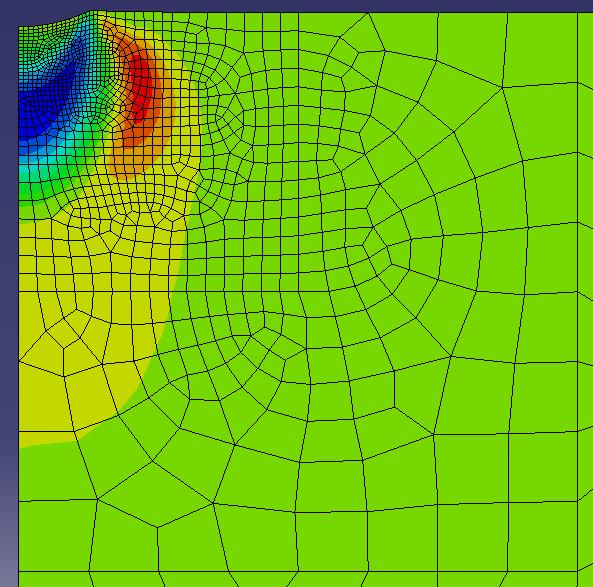
143 Figure B5: σ z stress contour for a five impact analysis using steel shot. Figure B6: σ r stress contour for a five impact analysis using steel shot. 13

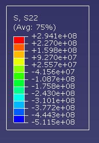
144 Figure B7: σ z stress contour for a ten impact analysis using steel shot. Figure B8: σ r stress contour for a ten impact analysis using steel shot. 14

145 Appendix C: D Axisymmetric Stress Contour Plots (Glass Shot) Figure C1: σ z stress contour for a single impact analysis using glass shot. Figure C: σ r stress contour for a single impact analysis using glass shot. 15

146 Figure C3: σ z stress contour for a double impact analysis using glass shot. Figure C4: σ r stress contour for a double impact analysis using glass shot. 16

147 Figure C5: σ z stress contour for a 5 impact analysis using glass shot. Figure C6: σ r stress contour for a 5 impact analysis using glass shot. 17

148 Figure C7: σ z stress contour for a 10 impact analysis using glass shot. Figure C8: σ z stress contour for a 10 impact analysis using glass shot. 18

149 Appendix D: D Cartesian ABAQUS Models with Uniform Shot Spacing Figure D1: The D Cartesian ABAQUS model used to simulate the case of a single row of 7 equally spaced shots impacting the target surface. Figure D: The D Cartesian ABAQUS model used to simulate the case of three rows of 7 equally spaced shots impacting the target surface. 19

150 Figure D3: The D Cartesian ABAQUS model used to simulate the case of six rows of 7 equally spaced shots impacting the target surface. 130

151 Appendix E: D Cartesian Stress Contour Plots (Uniformly Spaced Steel Shot) Figure E1: σ y stress contour for a 1 impact analysis using steel shot. Figure E: σ x stress contour for a 1 impact analysis using steel shot. 131

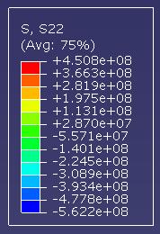
152 Figure E3: σ y stress contour for a 3 impact analysis using steel shot. Figure E4: σ x stress contour for a 3 impact analysis using steel. 13

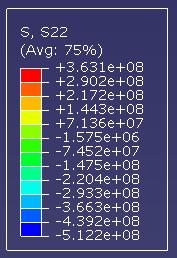
153 Figure E5: σ y stress contour for a 6 impact analysis using steel shot. Figure E6: σ x stress contour for a 6 impact analysis using steel shot. 133

154 Appendix F: D Cartesian Stress Contour Plots (Uniformly Spaced Glass Shot) Figure F1: σ y stress contour for a 1 impact analysis using glass shot. Figure F: σ x stress contour for a 1 impact analysis using glass shot. 134

155 Figure F3: σ y stress contour for a 3 impact analysis using glass shot. Figure F4: σ x stress contour for a 3 impact analysis. 135

156 Figure F5: σ y stress contour for a 6 impact analysis using glass shot. Figure F6: σ x stress contour for a 6 impact analysis using glass shot. 136

157 Appendix G: D Cartesian ABAQUS Models with Random Shot Spacing Figure G1: The D Cartesian ABAQUS model used to simulate the case of three rows of 7 randomly spaced shots impacting the target surface. 137

158 Figure G: The D Cartesian ABAQUS model used to simulate the case of six rows of 7 randomly spaced shots impacting the target surface. 138

159 Appendix H: D Cartesian Stress Contour Plots (Randomly Spaced Steel Shot) Figure H1: σ y stress contour for a 3 impact analysis using steel shot. Figure H: σ x stress contour for a 3 impact analysis using steel shot. 139

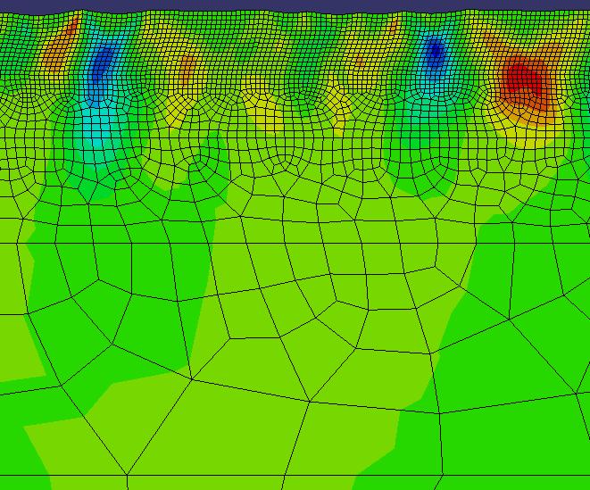
160 Figure H3: σ y stress contour for a 6 impact analysis using steel shot. Figure H4: σ x stress contour for a 6 impact analysis using steel shot. 140

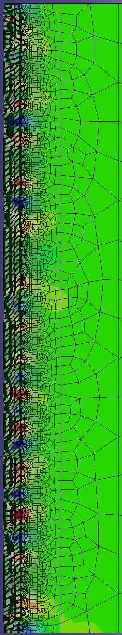
161 Figure H5: σy stress contour for a 3 impact analysis using steel shot. Figure H6: σx stress contour for a 3 impact analysis using steel shot. 141

162 Figure H7: σy stress contour for a 6 impact analysis using steel shot. Figure H8: σx stress contour for a 6 impact analysis using steel shot. 14

163 Appendix J: D Cartesian Stress Contour Plots (Randomly Spaced Glass Shot) Figure J1: σ y stress contour for a 3 impact analysis using glass shot. Figure J: σ x stress contour for a 3 impact analysis using glass shot. 143

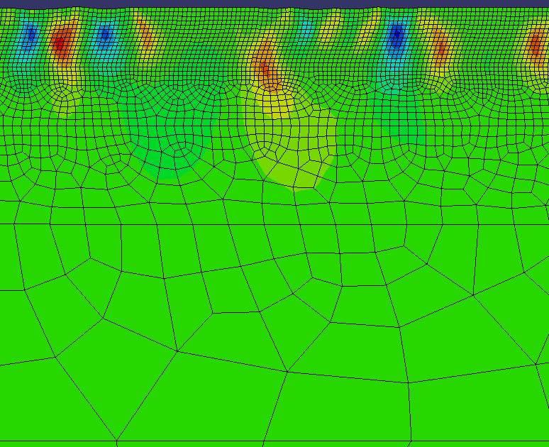
164 Figure J3: σ y stress contour for a 6 impact analysis using glass shot. Figure J4: σ x stress contour for a 6 impact analysis using glass shot. 144

165 Figure J5: σy stress contour for a 3 impact analysis using glass shot. Figure J6: σx stress contour for a 3 impact analysis using glass shot. 145

166 Figure J7: σy stress contour for a 6 impact analysis using glass shot. Figure J8: σx stress contour for a 6 impact analysis using glass shot. 146

167 Appendix K: ABAQUS Model Validation Studies Before building the ABAQUS models that were used for the research presented in this paper several validation studies were conducted. These studies were done with the intent of becoming familiar with the ABAQUS software, and at the same time, constructing meaningful models for which exact solutions exist. In the first couple of cases described in this appendix the results of the ABAQUS models were validated against exact solutions presented by Timoshenko [7] in his work Theory of Elasticity and Johnson s [8] Contact Mechanics. CASE 1: Load Distributed over a Part of the Boundary of a Semi-infinite Solid For this particular case the situation of a load distributed over a part of the boundary of a semi-infinite solid was modeled using ABAQUS and then compared to the exact solution as presented by Timoshenko [7] in his book, Theory of Elasticity. Given below is a general summary of the equations presented by Timoshenko followed by the results obtained from the ABAQUS analysis that was conducted. For further information on how the equations presented below were derived please refer to Theory of Elasticity by Timoshenko. Shown in Equations K1 and K below are the methods for calculating values of σ z, σ r, and σ θ. It is important to note that these equations all pertain to stress values along the central axis of the disk [7]. 3 z σ z = q 1+ (K1) ( ) a + z 3 3 q ( ) ( 1+ ν ) z z σ r = σ θ = 1+ ν + (K) a + z a + z 147

168 NOTE: q = Applied Load z = Depth from Surface ν = Poisson s Ratio a = Radius of Circle Defining Pressure Load In this particular situation a steel disk having properties ν = 0.3 and E = 00e9Pa was evaluated. A pressure load, q, of 150N/m was then distributed over a radius, a, of 0.1m on the upper most surface of the disk. Equations K1 and K were then loaded into a Microsoft Excel spreadsheet to produce values based on the depth from the surface of the plate ranging from 0m to 0.75m in 0.05m increments. The values given in Table K1 below represent the exact solution obtained using Timoshenko s equations and were the standard against which the ABAQUS models presented in this section were judged. 148

169 Table K1: Calculated stresses based on Timoshenko s equations. Depth, z σ z σ r = σ θ (m) Pa Pa Shown in Figure K1 below is the axisymmetric ABAQUS model that was created to represent the case of a load distributed over a part of the boundary of a semi-infinite solid. In this particular case the solid was given the dimensions 0.75m x 0.75m. These dimensions were dictated by the need to create a semi-infinite solid. Preliminary models were constructed to determine the best dimensions for the disk. In this particular case the best dimensions were those for which boundary effects did not exist. As one can see the pressure load of 150N/m was applied over a radius of 0.1m on the upper most surface of the disk while boundary conditions were applied to the central axis of the disk, as well as, to the bottom. Specifically, an XSYMM condition was used at the central axis in which U 1 = UR = UR 3 = 0. The boundary condition used for the bottom of the disk was U = UR 3 = 0. With all of the boundary conditions in place and the load applied as described it was then possible to begin meshing the model and performing the analysis. 149

170 Figure K1: Shown above is the axisymmetric ABAQUS model that was created in order to simulate the problem present by Timoshenko of a load distributed over a part of the boundary of a semi-infinite solid. For the first case a uniform mesh of 0.03m was used throughout the entirety of the disk. The results obtained are shown in Figures K and K3 with the first figure containing the stress in the z-direction and the second containing stress values in the r- direction. Listed in Table K are the exact stress values that were obtained along the central axis of the disk. In the second case and for the rest of the cases presented it was decided that a more refined mesh should be used. However, unlike the previous case in which a uniform mesh was used throughout the disk, it was determined that the best results could be obtained if the mesh was refined in steps with the finest mesh located near the surface where the pressure load was being applied. These areas of refinement are best shown in Figure K1. In this figure the smallest area has dimensions of 0.1m x m while the large refinement area has dimensions of 0.375m x 0.375m. For the second case that was 150

171 analyzed a mesh of 0.05m was used in the smallest area, 0.05m in the larger refinement area, and 0.1m for the remaining portion of the disk. The results that were obtained from this analysis are given in Figures K4 and K5 below with exact stress values presented in Table K3. For the third case a mesh of 0.01m was used in the smallest area, m in the larger refinement area, and finally a mesh of 0.075m was used throughout the remaining portion of the disk. The results obtained from this analysis are presented in Figures K6 and K7 below with exact stress values presented in Table K4. Finally, in the fourth case, a mesh size of m was used in the smallest area, while a 0.03m mesh was utilized in the larger refinement area, and then 0.06m throughout the remainder of the disk. Results based on this mesh arrangement are given in Figures K8 and K9 with exact stress values presented in Table K5. 151

172 Figure K: σ z Stress for a Uniform Mesh of 0.03m. Figure K3: σ r Stress for a Uniform Mesh of 0.03m. 15

173 Table K: Stress values obtained using ABAQUS and a uniform mesh of 0.03m. Depth, z σ z σ r = σ θ (m) (Pa) (Pa)

174 Figure K4: σ z Stress for a Varying Mesh of 0.1m, 0.05m, and 0.05m. Figure K5: σ r Stress for a Varying Mesh of 0.1m, 0.05m, and 0.05m. 154

175 Table K3: Stress values obtained using ABAQUS and a varying mesh of 0.1m, 0.05m, and 0.05m. Depth, z σ z σ r = σ θ (m) Pa Pa

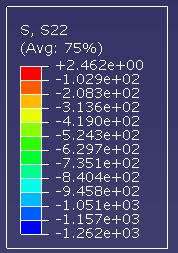
176 Figure K6: σ z Stress for a Varying Mesh of 0.075m, m, and 0.01m. Figure K7: σ r Stress for a Varying Mesh of 0.075m, m, and 0.01m. 156

177 Table K4: Stress values obtained using ABAQUS and a varying mesh of 0.075m, m, and 0.01m. Depth, z σ z σ r = σ θ (m) Pa Pa

178 Figure K8: σ z Stress for a Varying Mesh of 0.06m, 0.03m, and m. Figure K9: σ r Stress for a Varying Mesh of 0.06m, 0.03m, and m. 158

179 Table K5: Stress values obtained using ABAQUS and a varying mesh of 0.06m, 0.03m, and m. Depth, z σ z σ r = σ θ (m) Pa Pa

180 Having obtained a great deal of data at varying mesh sizes it was then necessary to compare this data against the exact solution presented by Timoshenko. In order to do this the L error norm method of comparison was utilized. Shown in Equation K3 below is the equation for calculating the L error norm. L = i= NOE ( exact ( i) σ calculated ( i) ) i= 1 σ (K3) Presented in Table K6 below are the L error norms for each of the cases described above. As one can see from viewing this data the L error norm decreased with each mesh refinement indicating that the results obtained slowly converged to the exact solution as given by Timoshenko. Table K6: L error norm values Mesh σ z σ r = σ θ 0.03m Uniform Mesh m, 0.05m, and 0.05m Varying Mesh m, m, and 0.01m Varying Mesh m, 0.03m, and m Varying Mesh Shown in Figures K10 and K11 are graphical representations of how the results obtained from the four different cases stack up against the values calculated using Timoshenko s equations. These graphs help to further demonstrate what the L norm calculations given in Table K6 above already did, which is that with each mesh refinement the stresses obtained from the ABAQUS analysis better represent the exact solution. 160

181 Stress (Pa) Timoshenko (z) Case 1 Case -100 Case 3 Case Depth from Surface (m) Figure K10: Above is a graph depicting σz vs. depth for each of the four cases presented above as well as the exact solution obtained by Timoshenko. 161

182 Stress (Pa) Timoshenko (r) Case 1 Case Case 3 Case Depth from Surface (m) Figure K11: Above is a graph depicting σr vs. depth for each of the four cases presented above as well as the exact solution obtained by Timoshenko. 16

183 CASE : Pressure Between Two Spherical Bodies in Contact Shown previously was the ability to apply a pressure load over a specific area and obtain results that were considered favorable when compared to the exact solution as obtained by Timoshenko. In this second case a Hertz contact problem was analyzed. This problem called for some of the same skills used in the previous case while expanding on them through the addition of contact. Results obtained using ABAQUS were compared to the exact solution as obtained by Johnson [8] in his work Contact Mechanics. Shown in Figure K1 below is a depiction of the specific case that was analyzed. As one can see this case is a more specific version of the one presented by Timoshenko in that there are no longer two spherical bodies in contact but rather one spherical body and a flat surface. Described in the following section are the modifications that were made to Timoshenko s equations in order to accommodate this change. Figure K1: Diagram showing spherical indenter contacting a flat surface. Shown in Table K7 below are both the material and physical properties for the flat surface and spherical indenter. It is important to note that because the specific type of indenter being used is a rigid one that its modulus of elasticity, E =. 163

184 Table K7: Material and physical properties. Property Flat Surface Rigid Indenter Poisson s Ratio ν 1 = 0.3 ν Modulus of Elasticity E 1 = 00E9 Pa E = Radius R 1 = R = 0.1 Given in Equations K4 and K5 below are the equations used to compute the material constants, k 1 and k, for the flat surface and spherical body respectively [7]. k k 1 1 ν 1 = (K4) πe 1 1 ν = (K5) πe By applying the material properties given in Table K7 to Equation K5 above one can see that the value for k << 1 which is in line with the assumption of a rigid spherical indenter. Given in Equation K6 below is the equation for calculating the radius of the surface of contact, a. In this case the applied load, P, was assigned a value of N. The reasoning behind this selection will be explained later in this section. Also, given in Equation K7 below is method for calculating the displacement, α [7]. a = 3 3π P 4 ( k + k ) 1 R1R R + R 1 (K6) 9π 16 ( k + k ) ( R R ) P + R R α = (K7) 1 With the above equations having been established it was then necessary to apply the assumptions given in Table K7 above, R 1 = and k << 1, to modify them so that they would work for the very specific case of a rigid spherical indenter in contact with a flat, 164

185 deformable surface. When these assumptions were applied to Equation K6 the result was Equation K8. a 3π 4 = 3 Pk1R (K8) At the same time, using the same assumptions in Equation K7 resulted in the below Equation K9 for calculating the displacement. 9π P k 3 1 α = (K9) 16 R Finally, having established equations for both the radius of the surface of contact and the displacement all that remained was an equation for calculating the maximum pressure load on the flat surface, q 0. Values of q 0 can be obtained using Equation K10 below [7]. q 0 3P = (K10) πa Because the ABAQUS model was created in such a way that a specific displacement, 0.001m, was assigned to the rigid indenter it was necessary to determine the exact load that this displacement was equated to. In doing so, Equation K9, was rearranged to solve for the load, P. The resulting equation is given below in Equation K R P = α 3 k (K11) π 1 Shown in Equations K1 and K13 below are the methods used to calculate the stresses along the central axis of the disk at varying depths. These equations were taken from Johnson s book, Contact Mechanics. From these equations the values given in Table K8 were computed. These represent the exact stress values for the case of a rigid 165

186 166 spherical indenter contacting a deformable, flat surface and are the values against which the ABAQUS obtained stresses were compared [8] = a z q z σ (K1) ( ) = = tan 1 1 a z z a a z q r ν σ σ θ (K13)

187 Table K8: Calculated Stresses from Johnson Depth, z σ z σ r = σ θ (m) (Pa) (Pa) E E E E E E E E E E E E E E E E E E E E E E E E E E E E E E E E E E E E E E E E E E E E E E E E E E E E

188 With an exact solution in place the next task was to establish an ABAQUS model. Shown in Figure K13 below is the ABAQUS model that was created. In this particular case the disk section shown was given the dimensions 0.75m x 0.75m. Boundary conditions were applied to the central axis of the disk, as well as, to the bottom. Specifically an XSYMM condition was used at the central axis in which U 1 = UR = UR 3 = 0. The boundary condition used for the bottom of the disk was U = UR 3 = 0. Boundary conditions were also applied to the reference point, designated with an RP in Figure K13, of the rigid indenter. To this point an XSYMM boundary condition, as well as, a displacement of m in the y-direction were applied. In viewing the model one will also notice that the disk has been partitioned into 4 different areas. This was done so that the applied mesh can be refined around the contact area while remaining relatively course in the part of the disk furthest from the contact area. Figure K13: Shown above is the axisymmetric ABAQUS model that was created into to simulate the specific case of a rigid spherical indenter contacting a deformable, flat surface. 168

189 In the first analysis a varying mesh of 0.1m, 0.05m, 0.05m, and 0.005m was used in the four mesh refinement areas with the largest mesh being furthest from the contact area and the finest mesh located directly around the area of contact. Results based on this level of mesh refinement are shown in Figures K14 and K15 with exact values presented in Table K9. For the purpose of clarity Figures K14 and K15 have been cropped so that only the most refined mesh is represented. In the second analysis a varying mesh of 0.5m, 0.1m, 0.05m, and 0.004m was used in the four mesh refinement areas. Of particular significance is the decreased size in the mesh directly around the area of contact which was refined from 0.005m in the first analysis to 0.004m for this second analysis. The finer mesh helped to produce better results, which are shown in Figures K16 and K17. Exact stress values have been tabulated in Table K10. For the third analysis the mesh was set to 0.5m in the three largest mesh refinement areas with a mesh of 0.003m being utilized in the smallest mesh refinement area located directly around the contact surface. The even greater refinement in mesh around the contact area yielded slightly better results than those presented in the previous analysis using the 0.004m mesh around the contact surface. Results are given in Figures K18 and K19 below. Exact stress values are presented in Table K11. In order to facilitate a comparison of the data presented above against the exact stress values computed using Johnson s equations the graphs shown in Figures K0 and K1 were created. Figure K0 contains values of σ z vs. depth while Figure K1 shows σ r vs. depth. These graphs serve to validate the ABAQUS model for 3D axisymmetric indentation of a deformable surface by a rigid spherical indenter in demonstrating that the results obtained using this model very closely represent the exact solution as computed using Johnson s equations for calculating stresses along the central axis of the disk. 169

190 Figure K14: σ z Stress for a Varying Mesh of 0.1m, 0.05m, 0.05m, and 0.005m. Figure K15: σ r Stress for a Varying Mesh of 0.1m, 0.05m, 0.05m, and 0.005m. 170

191 Table K9: Stress values obtained using ABAQUS and a varying mesh of 0.1m, 0.05m, 0.05m, and 0.005m. Depth, z σ z σ r = σ θ (m) (Pa) (Pa) E E E E E E E E E E E+08.94E E+08.18E E E E E E E E E E E E E E E E+07 5.E E E E E E E E+07.7E E+07.16E E+07.16E E+07.15E E+07.15E E+07.14E E+07.10E E+07.03E

192 Figure K16: σ z Stress for a Varying Mesh of 0.5m, 0.1m, 0.05m, and 0.004m. Figure K17: σ r Stress for a Varying Mesh of 0.5m, 0.1m, 0.05m, and 0.004m. 17

193 Table K10: Stress values obtained using ABAQUS and a varying mesh of 0.5m, 0.1m, 0.05m, and 0.004m. Depth, z σ z σ r = σ θ (m) (Pa) (Pa) E E E E E E E E E E E E E+08.31E E E E E E E E E E E E E E E E E E+07.16E E E E E E E E E E E E E E E E E E E

194 Figure K18: σ z Stress for a Varying Mesh of 0.5m and 0.003m. Figure K19: σ r Stress for a Varying Mesh of 0.5m and 0.003m. 174

195 Table K11: Stress values obtained using ABAQUS and a varying mesh of 0.5m and 0.003m. Depth, z σ z σ r = σ θ (m) (Pa) (Pa) 0-1.E E E E E E E E E E E E E E E E E E E E E E E E E E E E E E E E E E E E E E E E E E E

196 Stress vs. Depth (0.001m Displacement) 0.00E E E E E+09 Stress (Pa) -1.00E E+10 Case 1 (z) Case (z) Case 3 (z) -1.40E+10 Johnson (z) -1.60E+10 Depth from Surface (m) Figure K0: Shown above is a plot of σz vs. depth for the 3 cases presented above. These cases are then compared to the σz stresses obtained through the use of Johnson s equations. 176

197 Stress vs. Depth (0.001m Displacement).00E E E E+09 Stress (Pa) -6.00E E+09 Case 1 (r) Case (r) -1.00E+10 Case 3 (r) Johnson (r) -1.0E+10 Depth from Surface (m) Figure K1: Shown above is a plot of σr vs. depth for the 3 cases presented above. These cases are then compared to the σr stresses obtained through the use of Johnson s equations. 177

198 Having viewed the data presented in Figures K0 and K1 one can see that while the ABAQUS data slowly converged on the correct solution there was still some error. Due to this error it was decided that an even greater level of mesh refinement was necessary in order to obtain the best results from the ABAQUS analysis. To facilitate the obtainment of more accurate results, a fifth level of mesh refinement was created directly around the contact surface having dimensions of 0.05m x 0.05m. The modified ABAQUS model is depicted in Figure K. Figure K: Shown above is the axisymmetric ABAQUS model that was created into to simulate the specific case of a rigid spherical indenter contacting a deformable, flat surface. Based on this new level of mesh refinement exact stress values were calculated based on Johnson s equations and a depth of up 0.05m in 0.00m increments. These stress values are given in Table K1 below. 178

199 Table K1: Calculated Stresses from Johnson Depth, z σ z σ r = σ θ (m) (Pa) (Pa) E E E E E E E E E E E E E E E E E E E E E E E E E E E E E E E E E E E E E E E E E E E E E E E E E E E E

200 With the new level of mesh refinement in place three more analyses were conducted. For the first ABAQUS analysis a mesh of 0.00m was utilized directly around the area of contact. The results of this analysis are shown in Figures K3 and K4. Once again, for the purpose of clarity, these figures have been cropped to only show the area directly around the contact surface. The exact stress values that were obtained for stresses along the central axis of the disk are given in Table K13. The mesh was then further refined to 0.001m in area directly around the contact surface for the second analysis. Results for the stress in the z-direction are shown in Figure K5 while results for stress in the r-direction are shown in Figure K6. Since these figures do not offer exact stress values along the axis of the disk Table K14 was inserted to better display the data. As a final attempt to obtain the best possible results a super fine mesh was created in the area directly around the contact surface. This mesh was half the size of the previous 0.001m or m in size. Results for stresses in the z-direction are displayed in Figure K7 followed by stress results in the r-direction which are shown in Figure K8. Finally, exact stress values are tabulated in Table K15. As was done with the coarser mesh results presented previously the results obtained using the finer level of mesh refinement were compared graphically to the exact values obtained using Johnson s equations. This graph is given in Figure K9 and contains data for stress in the z-direction, as well as, data for stress in the r-direction. As one can see from looking at this graph the results obtained for both σ z and σ r are very close to the exact solution presented by Johnson. This served as a very good indication that the model that was created could be used in further analyses where contact elements are present. 180

201 Figure K3: σ z Stress for a 0.00m mesh directly around the area if contact. Figure K4: σ r Stress for a 0.00m mesh directly around the area if contact. 181

202 Table K13: Stress values obtained using ABAQUS and a mesh of 0.00m directly around the contact area. Depth, z σ z σ r = σ θ (m) (Pa) (Pa) E E E E E E E E E E E E E E E E E E E E E E E E E E E E E E E E E E E E E E E E E E E E E+08.93E E E E E E E+07 18

203 Figure K5: σ z Stress for a 0.001m mesh directly around the area if contact. Figure K6: σ r Stress for a 0.001m mesh directly around the area if contact. 183

204 Table K14: Stress values obtained using ABAQUS and a mesh of 0.001m directly around the contact area. Depth, z σ z σ r = σ θ (m) (Pa) (Pa) E E E E E E E E E E E E E E E E E E E E E E E E E E E E E E E E E E E E E E E E E E E E E E E E E E E E

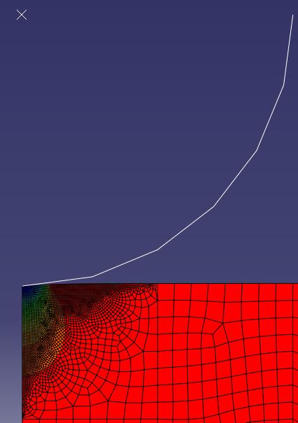
205 Figure K7: σ z Stress for a m mesh directly around the area if contact. Figure K8: σ r Stress for a m mesh directly around the area if contact. 185

206 Table K15: Stress values obtained using ABAQUS and a mesh of m directly around the contact area. Depth, z σ z σ r = σ θ (m) (Pa) (Pa) E E E E E E E E E E E E E E E E E E E E E E E E E E E E E E E E E E E E E E E E E E E E E E E E E E E+08.74E

207 Stress vs. Depth (0.001m Displacement) 1.000E E E E E+09 Stress (Pa) Case 1 (z) E+09 Case (z) Case 3 (z) Johnson (z) E+10 Case 1 (r) Case (r) Case 3 (r) E+10 Johnson (r) E+10 Depth from Surface (m) Figure K9: Shown in the graph above is a plot of both σz vs. depth and σr vs. depth for the 3 cases presented previously. These cases are then compared graphically to the exact solutions obtained using Johnson s equations. 187

208 Case 3: Plastic Model Validation through Mesh Refinement Having obtained an accurate model for the indentation of an elastic steel disk using a rigid spherical indenter the next step was to obtain a model that would be even more relevant to the research being conducted. In this case the next step was two fold. Because T-6Al-4V is the material that will be studied it was decided that now would be the best time to establish the necessary material properties for T-6Al-4V and enter them into the ABAQUS FEA software. Previous cases used steel as the material for the disk. The second part of this case involved expanding on the simple elastic material model that had been used up to this point by introducing the element of plasticity to the indentation model. In this case the results obtained for the plastic analysis of a disk made from T-6Al- 4V being indented by a rigid, spherical indenter will be validated through the process of mesh refinement. Through the use of gradual mesh refinement the hope was that the results obtained from the ABAQUS analysis would eventually converge. It is the convergence of the results that would signify that an accurate material model has been created with which accurate plastic analysis results can be obtained. For this study five different meshes were used varying from relatively course to extremely fine. In creating the material model for the plastic analysis the elastic properties of Table K16 were used in combination with the plastic properties given in Table K17. The Johnson-Cook hardening law using the rate-dependent option was utilized in creating the plastic material model for T-6Al-4V. Table K16: Elastic Properties for T-6Al-4V [5] ρ E ν (kg/m 3 ) (GPa) Ti-6Al-4V

209 Table K17: New Parameters For Johnson-Cook Material Model [4] A B n C m ε& T 0 melt T transition (MPa) (MPa) (s -1 ) ( C) ( C) Ti-6Al-4V Shown in Figure K30 below is the ABAQUS model that was created for use in this study. This is the same model that was utilized in the previous study in which elastic analyses of a rigid spherical indenter being pressed into a deformable, steel disk were validated. Since the model has already been validated and proven accurate it made sense to use it again for this study as the control in the experiment while the new plastic material model acted as the new variable. For more information regarding this model, as well as, the applied boundary condition refer to the previous study. Figure K30: Shown above is the ABAQUS model that was created for the purpose of the plastic material model validation study. 189

210 Shown in Figure K31 and Figure K3 are the results for the first analysis that was conducted. For this analysis a varying mesh of 0.5, 0.1, 0.05 and 0.005m was used. These figures have been cropped so that only two of the mesh refinement areas are depicted. In this case the 0.005m mesh was applied to both mesh refinement areas located directly around the contact surface. This analysis represents the coarsest mesh that was used for this particular case with the remaining analyses using progressively finer meshes around the contact surface. The exact values obtained for stress in the z- direction and stress in the r-direction are given in Table K18. For the second analysis a mesh of 0.004m was applied to the two mesh refinement areas located directly around the contact surface. Contrast plots of both stress in the z- direction and stress in the r-direction are given in Figure K33 and Figure K34 respectively. Exact values are tabulated in Table K19. Since in the previous two analyses the majority of the stress variation took place within the first mesh refinement area it was decided that for the final three analyses that only the mesh within this area would continue to be refined. For this analysis the vary mesh was set at 0.5, 0.1, 0.05, and 0.00m. The mesh directly around the contact surface was therefore reduced by 50%. Figures K35 and K36 show the contrast plots for stress in the z-direction and r-direction respectively. Exact values are listed in Table K0. For the fourth analysis the mesh directly around the contact surface was again reduced by 50% from the previous analysis to 0.001m. Stress plots for this analysis are given in Figure K37 and K38 and the exact stresses along axis of the disk are given in Table K1. Finally for the fifth and final analysis a mesh size of m was utilized in the area directly around the contact surface. Stress plots from this analysis are given in Figures K39 and K40 with exact stress values tabulated in Table K. Figure K39 and Figure K40 have been cropped such that only the finest mesh refinement area is shown. In order to best summarize the data that was collected over the course of the five analyses described above the plots shown in Figure K41 and Figure K4 were created. Figure K41 contains solely data for stress in z-direction while Figure K4 depicts data for stress in the r-direction. As one can see from viewing each of these plots the data 190

211 obtained does appear to converge by the final analysis. This is a very good indication that the plastic material model is in fact a valid one and can be used for future analyses in which Ti-6Al-4V will be the primary material of interest. 191

212 Figure K31: σ z Stress for a Varying Mesh of 0.5, 0.1, 0.05 and 0.005m. Figure K3: σ r Stress for a Varying Mesh of 0.5, 0.1, 0.05 and 0.005m. 19

213 Table K18: Stress values obtained using ABAQUS and a varying mesh of 0.5, 0.1, 0.05 and 0.005m. Depth, z σ z σ r = σ θ (m) (Pa) (Pa) E E E E E E E E E E E E E E E E E E E E E E E E E E E E E E E E E E E E E E E E E E E E E E E E E+07.80E E E

214 Figure K33: σ z Stress for a Varying Mesh of 0.5, 0.1, 0.05 and 0.004m. Figure K34: σ r Stress for a Varying Mesh of 0.5, 0.1, 0.05 and 0.004m. 194

215 Table K19: Stress values obtained using ABAQUS and a varying mesh of 0.5, 0.1, 0.05 and 0.004m. Depth, z σ z σ r = σ θ (m) (Pa) (Pa) E E E E E E E E E E E E E E E E E E E E E E E+08.7E E E E E E E E E E E E E E E E E E E E E E E E E E E E E

216 Figure K35: σ z Stress for a Varying Mesh of 0.5, 0.1, 0.05, and 0.00m. Figure K36: σ r Stress for a Varying Mesh of 0.5, 0.1, 0.05, and 0.00m. 196

217 Table K0: Stress values obtained using ABAQUS and a varying mesh of 0.5, 0.1, 0.05, and 0.00m. Depth, z σ z σ r = σ θ (m) (Pa) (Pa) E E E E E E E E E E E E E E E E E E E E E E E+08.91E E E E E E E E E E E E E E E E E E E E E E E E E E E E E

218 Figure K37: σ z Stress for a Varying Mesh of 0.5, 0.1, 0.05, and 0.001m. Figure K38: σ r Stress for a Varying Mesh of 0.5, 0.1, 0.05, and 0.001m. 198

219 Table K1: Stress values obtained using ABAQUS and a varying mesh of 0.5, 0.1, 0.05, and 0.001m. Depth, z σ z σ r = σ θ (m) (Pa) (Pa) E E E E E E E E E E E E E E E E E E E E E E E E E E E E E E E E E E E E E E E E E E E E E E E E E E E E

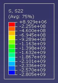
220 Figure K39: σ z Stress for a Varying Mesh of 0.5, 0.1, 0.05, and m. Figure K40: σ r Stress for a Varying Mesh of 0.5, 0.1, 0.05, and m. 00

221 Table K: Stress values obtained using ABAQUS and a varying mesh of 0.5, 0.1, 0.05, and m. Depth, z σ z σ r = σ θ (m) (Pa) (Pa) E E E E E E E E E E E E E E E E E E E E E E E+08.91E E E E E E E E E E E E E E E E E E E E E E E E E E E E+07.98E+06 01

222 Stress vs. Depth (0.001m Displacement) 0.000E E E E+09 Stress (Pa) -.000E+09 Case 1 (z) Case (z) -.500E+09 Case 3 (z) Case 4 (z) Case 5 (z) E+09 Depth from Surface (m) Figure K41: A graph depicting the results of the five analyses conducted for stresses in the z-direction. 0

223 Stress vs. Depth (0.001m Displacement) 4.000E E E E E E E+08 Stress (Pa) E E+09 Case 1 (r) E+09 Case (r) Case 3 (r) E+09 Case 4 (r) Case 5 (r) E+09 Depth from Surface (m) Figure K4: A graph depicting the results of the five analyses conducted for stresses in the r-direction. 03

224 Case 4: Elastic vs. Plastic Stresses for Indentation of Ti-6Al-4V For this particular case the results obtained from a plastic analysis of the indentation of a disk made of T-6Al-4V were compared to the results from an elastic analysis of the indentation of a disk made from T-6Al-4V. In the cases described previously it was shown that for both elastic and plastic analyses having an extremely fine mesh directly around the contact surface yielded the best results. Because of this a varying mesh of 0.5, 0.1, 0.05, 0.015, and m was selected for the five mesh refinement areas. Given in Figure K43 is a depiction of the model that was used for both the elastic analysis, as well as, the plastic analysis showing the indenter, disk, and the applied boundary conditions. This is the same model that was validated earlier in Case of Appendix K. Boundary conditions were applied to the central axis of the disk, as well as, to the bottom. Specifically, an XSYMM condition was used at the central axis in which U 1 = UR = UR 3 = 0. The boundary condition used for the bottom of the disk was U = UR 3 = 0. Boundary conditions were also applied to the reference point, designated with an RP in Figure K43, of the rigid indenter. To this point an XSYMM boundary condition, as well as, a displacement of m in the y-direction were applied. 04

225 Figure K43: Shown above is the model that was used for both the elastic and plastic analysis. The elastic analysis was conducted first. Shown in Figure K44 are ABAQUS results for stress in the z-direction while Figure K45 depicts the stresses in the r-direction. Exact values for these stresses are tabulated in Table K3. Depicted in Figure K46 and Figure K47 are the σ z and σ r stresses respectively that resulted from the plastic analysis. Listed in Table K4 are the exact stress values for the plastic case. In order to best summarize and compare the data that was collected from both the elastic and plastic analysis the graph shown in Figure K48 was created. As one can see from looking at this graph the results obtained follow the accepted theory that stress values obtained using the elastic material model should be greater than those obtained from the elastic-plastic material model. This result helps to further validate the results that were obtained in the previous two cases in this appendix. 05

226 Figure K44: σ z Stress for a Varying Mesh of 0.5, 0.1, 0.05, and m using the elastic material model. Figure K45: σ r Stress for a Varying Mesh of 0.5, 0.1, 0.05, and m using the elastic material model. 06

227 Table K3: Stress values obtained using ABAQUS and a Varying Mesh of 0.5, 0.1, 0.05, and m using the elastic material model. Depth, z σ z σ r = σ θ (m) (Pa) (Pa) E E E E E E E E E E E E E E E E E E E E E+08.14E E E E E E E E E E E E E E E E E E E E E E E E E E E E E E E+06 07

228 Figure K46: σ z Stress for a Varying Mesh of 0.5, 0.1, 0.05, and m using the plastic material model. Figure K47: σ r Stress for a Varying Mesh of 0.5, 0.1, 0.05, and m using the plastic material model. 08

229 Table K4: Stress values obtained using ABAQUS and a Varying Mesh of 0.5, 0.1, 0.05, and m using the plastic material model. Depth, z σ z σ r = σ θ (m) (Pa) (Pa) E E E E E E E E E E E E E E E E E E E E E E E+08.91E E E E E E E E E E E E E E E E E E E E E E E E E E E E+07.98E+06 09

230 Stress vs. Depth (0.001m Displacement) 1.000E E E E E E+09 Plastic Stress (Pa) E E+09 Elastic (z) Elastic (r) E+09 Plastic (z) E+09 Plastic (r) E+09 Depth from Surface (m) Figure K48: A graph depicting the contrast between the elastic and plastic results obtained. 10

231 Case 5: Dynamic Impact Analysis In the previous cases described in this appendix an ABAQUS model has been established which was validated for both elastic and plastic material properties. In each case this model was validated based on the condition of a 1mm displacement being imposed on the target disk by a rigid, spherical indenter having a radius of 0.1m. However, shot peening by definition is a dynamic process in which the shot is propelled at the target to be peened at a set velocity. In this case three dynamic impact models were created simulating 1,, and 5 impact(s) on the surface of the target material. These models are shown in Figure K49 through K51 below. The boundary conditions used are identical to the ones utilized in the previous cases describe in this appendix. Figure K49: The ABAQUS model above was used to simulate the single impact of a rigid spherical indenter against the target disk. The applied boundary conditions are also shown. 11

232 Figure K50: The ABAQUS model above was used to simulate the double impact of a rigid spherical indenter against the target disk. The applied boundary conditions are also shown. Figure K51: The ABAQUS model above was used to simulate 5 impacts of a rigid spherical indenter against the target disk. The applied boundary conditions are also shown. Unlike the previous cases described in this appendix in which the mass of the indenter was insignificant due to the specified indentation depth it was necessary in this case to assign a mass to the indenter. A point mass of 3.9kg was assigned to the indenter at its geometric center of mass. This value was based on the use of a steel shot material having a density of 7860kg/m 3 and an indenter radius of 0.1m. For the 1,, and 5 impact models all of the indenters were assigned an initial velocity of 55m/s. This corresponds to the average shot velocity typically used during peening operations. 1

233 In the first analysis a single impact of a shot with the target material was simulated. Shown in Figure K5 and Figure K53 are the stress contours for stress in the z-direction and r-direction respectively. These contours represent the residual stresses present in the disk after just a single indent. As was done in the previous cases described in this appendix stress data was obtained along the central axis of the disk. Exact stress values were obtained from the surface of the disk to a depth of 0.375m or half the thickness of the disk in 0.005m increments. A summary of this data is presented in Table K5 in 0.05m increments. The second analysis that was conducted involved simulating two impacts of the shot with the target material. Contour plots of σ z and σ r are given in Figure K54 and K55 respectively. A summary of the exact stress values obtained is given in Table K6. Finally, an analysis was conducted in which the target material was impacted 5 times by the shot. The resulting stress contours are given in Figure K56 and K57 for σ z and σ r respectively. Exact stress values are given in Table K7. In order to provide the best possible means of summarizing the data that was collected the plots shown in Figure K58 and Figure K59 were created. Shown in Figure K58 is a plot of σ z vs. depth from the surface of the target along the central axis of the disk. In general one can see that while the magnitude of the maximum compressive stress remains almost constant across the three different analyses the depth at which it occurs in the disk increases with each impact. A similar trend is also exhibited for stress in the r-direction plotted in Figure K59 against depth from the surface of the target. 13

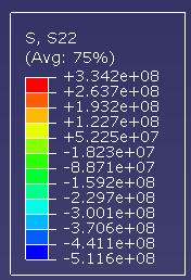
234 Figure K5: Shown above is the σ z stress contour plot based on the single impact analysis that was conducted using ABAQUS and a varying mesh of 0.5, 0.1, 0.05, and m. Figure K53: Shown above is the σ z stress contour plot based on the single impact analysis that was conducted using ABAQUS and a varying mesh of 0.5, 0.1, 0.05, and m. 14

235 Table K5: Shown below are the exact values for σ z and σ r based on the single impact analysis conducted using ABAQUS and a varying mesh of 0.5, 0.1, 0.05, and m. Depth, z σ z σ r = σ θ (m) (Pa) (Pa) E E E E E E E E E E E E E E E E E E E E E E E E E E E E E E E E+06 15

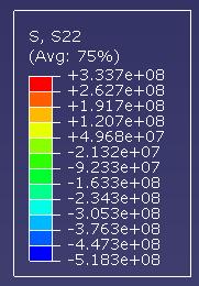
236 Figure K54: Shown above is the σ z stress contour plot based on the double impact analysis that was conducted using ABAQUS and a varying mesh of 0.5, 0.1, 0.05, and m. Figure K55: Shown above is the σ r stress contour plot based on the double impact analysis that was conducted using ABAQUS and a varying mesh of 0.5, 0.1, 0.05, and m. 16

237 Table K6: Shown below are the exact values for σ z and σ r based on the double impact analysis conducted using ABAQUS and a varying mesh of 0.5, 0.1, 0.05, and m. Depth, z σ z σ r = σ θ (m) (Pa) (Pa) E E E E E E E E E E E E E E E+07.30E E E E E E E E E E E E E E E E E+06 17

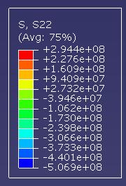
238 Figure K56: Shown above is the σ z stress contour plot based on an analysis having 5 impacts that was conducted using ABAQUS and a varying mesh of 0.5, 0.1, 0.05, and m. Figure K57: Shown above is the σ r stress contour plot based on an analysis having 5 impacts that was conducted using ABAQUS and a varying mesh of 0.5, 0.1, 0.05, and m. 18